
Abstract
In guided wave (GW)-based structural health monitoring (SHM), ultrasonic elastic waves are used to detect damages in structures by comparing the acquired signals with those acquired before defect formation. Making the SHM system automatic, especially for similar structures, such as turbine blades, is rather challenging. The high sensitivity of GWs to environmental and operational conditions, the variabilities due to sensor positioning, sensor coupling, and material variability in composites limit the baseline application. This work presents a machine learning (ML)-based damage detection method using aggregated baselines independent of their damaged states to enhance the generalization capability of ML algorithms by considering similar structures’ variabilities. The methodology relies on feature extraction from raw GW signals and training classification algorithms (e.g., kernel machines, ensemble methods, and neural networks). Two experimental data sets on composite panels are used. The first experimental data set of 45 composite panels is used to validate the approach by considering the aforementioned inter-specimen variabilities. Half of the 45 panels provide pristine data, and the rest provide damaged data so that the same sample is present in the training or test set but never in both. High classification performance is obtained, demonstrating that the classifier has successfully learned to recognize defect signatures despite the influence of the variabilities linked to the multiple instrumented specimens. The second experimental data set of 1 composite panel with temperature variation is used. Good classification performance is obtained without using baseline correction methods.
Keywords
Introduction
Structural health monitoring (SHM) is implementation of damage detection strategies for structures by means of permanently embedded sensors acquiring information seamlessly. 1 This information is later processed to diagnose the state of the structure. Different types of SHM systems have already been proposed; among them are vibration-based and guided wave-based SHM (GW-SHM). 2 The latter uses ultrasonic sound waves for inspection, which can travel long distances and are highly sensitive to defects. The potential areas of GW application are pipeline inspection (oil and gas industries), bridges, and aircraft structures.
In GW-SHM, a pair of piezoelectric transducers are used; one acts as an emitter and the other as a receiver placed away from the emitter. The emitted GWs interact with the defect, which causes changes to the waveform, such as, change in amplitude and/or change in phase. 3 This change in the signals is then identified by subtracting the acquired signal with a reference signal measured on undamaged state. The resulting residual signal is the indication of the presence of a defect; this approach is called baseline subtraction. 3 However, GWs are not just sensitive to defects but also to environmental and operational conditions, material properties, and transducer coupling; for example, increasing temperature reduces the stiffness of the material that in turn changes the wave speed. Hence, the variation in the temperature of the current state must be limited to ensure the reliability of baseline subtraction method. Along with temperature, other influences on GW propagation are listed in the study by Gorgin et al. 4 With the influence of aforementioned factors, baseline subtraction becomes ineffective.
The literature offers numerous baseline correction methods that mainly focus on temperature compensation. Optimal baseline selection, 5 is one in which the residual signal amplitude is minimized until an optimal baseline is selected from the pool of acquired baselines. In baseline signal stretch technique proposed by Croxford et al., 6 the current signal is stretched until it matches with the baseline. A big pool of baselines is required for optimal baseline selection method which is not practical, and baseline signal stretch alters the frequency content of the signal which is not effective for higher temperatures. 4 Other proposed methods are, combination of the above two methods 7 and dynamic time warping. An optimal mapping between two time series with changing amplitude or speed is determined in dynamic time warping. 8 Other temperature compensation methods requiring a baseline/a set of baselines include those given under references.9–12 The efficiency of these methods degrades when the temperature of the test specimen is beyond the range considered for acquiring baselines. 13 Improved baseline signal stretch methods listed in the review paper by Gorgin et al. 4 can be effective for a temperature difference of 18°C. Kulakovskyi 14 showed in his thesis that, dynamic time warping is effective for a temperature difference of up to 25°C. The aforementioned methods, however, employ alignment of the baseline signals, and their main focus is temperature compensation alone, but other environmental conditions, sensor variability, and so on also affect GW signals. 4
Baseline-free approaches have been proposed to overcome the baseline dependency. Time reversibility of lamb waves, 15 transfer impedance of transducers, 16 cross-correlation analysis proposed by Alem et al. 17 are some of the baseline-free methods listed in the review paper by Gorgin et al. 4 The baseline-free techniques utilize mainly the signal energy, and because environmental and operational conditions also modify the amplitude of the signal, these techniques become less effective. 4 In recent times, the use of machine learning (ML) and deep learning is increasing in defect detection and localization in GW-SHM. Miorelli et al.18,19 employed post-processed GW-imaging to train kernel machines, but ultrasound- and GW-based images are constructed using residual states obtained from baseline subtraction. Schnur et al. 20 worked on the detection of temperature-affected signals using standard classifiers and features. However, the temperature effect was compensated through optimal baseline selection and baseline signal stretch. Rautela et al. 21 showed good classification performance on a composite panel using a One-Dimensional Convolutional Neural Network (NN). The aforementioned works depend on baseline correction and do not present the study on the robustness of the developed methodology concerning similar structures or when baselines are unavailable.
ML-based damage detection in GW-SHM results in a configuration-specific monitoring scheme, which means that the structure on which a ML model is trained cannot be used for the diagnosis of other similar structures, let alone other arbitrary structures. To achieve a real-time automatic monitoring GW-SHM system for similar structures, the generalization capability of ML models needs to be enhanced. It can be accomplished by taking into account the inter-specimen variability across multiple similar instrumented structures. These variabilities include material properties, sensor position, sensor coupling, defect location, shape and size, and environmental and operational conditions. The main goal of this work is to develop a robust damage detection scheme for similar structures.
To conduct the research, we considered two distinct data sets. The first one (in-house measurement data set) contains inter-specimen variabilities as a result of measurement data coming from 45 carbon fiber reinforced polymer (CFRP) panels and has minor temperature variation (i.e., 20 ± 2°C). Therefore, the Open guided wave (OpenGW) data set 22 is considered, which contains more significant temperature variation (i.e., [20°C, 60°C]). The methodology consists of baseline aggregation, AutoRegression (AR) for extracting features from the signals under the influence of variabilities without correcting the baselines and classification. The supervised ML classifiers are used to classify the two states. Furthermore, variability inclusion through multiple structures aid in improving the generalization capability of ML models. The most recent works on the OpenGW data set include applying baseline correction methods to compensate for temperature effect. 20 And Abbassi et al. 23 perform damage classification without relying on baseline correction but consider temperature groups with shorter ranges (i.e., 10°C temperature difference). We conducted the study on the OpenGW data set by applying AR modeling and baseline aggregation methodology to avoid using baseline correction methods and considering temperature groups with a more comprehensive temperature range (i.e., up to 40°C).
Experimental setup and data description is first presented in methodology section. Then data annotation process is explained, in which significant defect information-carrying signals in damaged panels are separated from those carrying less significant information. The following section explains baseline aggregation procedure. Then feature extraction process, experimental validation, discussion, and conclusion are presented in the subsequent sections.
Methodology
Data description
The experimental set up consists of 45 CFRP panels. Each of the panels is instrumented with 6 PZT transducers distributed over a 150-mm radius circle, one sample instrumented panel is shown in Figure 1. In this experiment, delamination type defects are induced by means of impacting each panel with a 16-mm radius steel head and no second impact was allowed. The 45 panels are impacted at different locations within the circle defined by the sensor network.
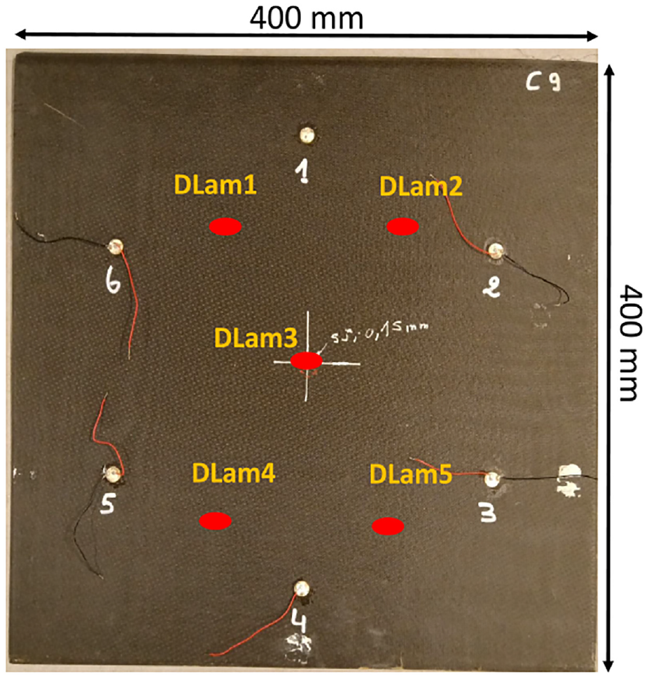
A sample CFRP panel of size 400mm × 400 mm instrumented with six PZT sensors. The elliptical marker (①) shows five delamination locations (i.e., DLam1, DLam2, DLam3, DLam4, and DLam5). Note that the delamination is present at either one of the five locations given a single panel.
GWs were generated by using a two-cycles tone burst waveform and four excitation frequencies namely, 40, 60, 80, and 100 kHz are used for measurement. The size of the delamination to be detected drives frequency selection. But for higher frequencies, multiple modes exist, and there is an overlap of modes, which does not allow for the extraction of proper time of flight (ToF) information. Therefore the four frequencies’ selection is a trade-off between damage detectability and mode overlap. Signal acquisition was carried out by exciting the transducers in round robin fashion, thereby acquiring 15 unique signals per panel at a sampling frequency of 5 MHz.
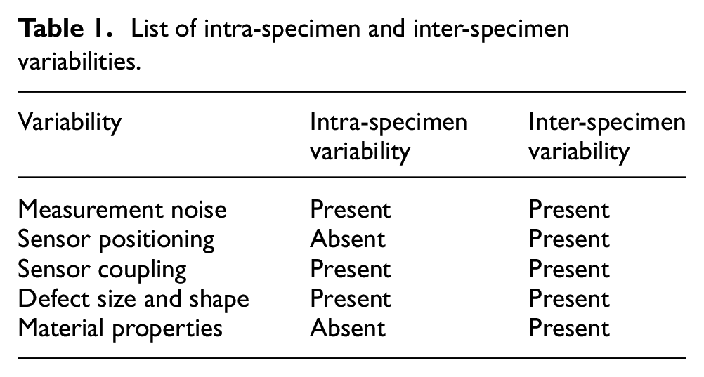
Signal acquisition was first completed on 45 pristine panels. Later, the impact-caused delamination of varying sizes and at either one of the five different locations as shown in Figure 1 were created on all 45 panels, and damaged state signals were acquired. Three sample signals of shortened length are shown in Figure 2 to illustrate the complexity in the signals caused by intra- and inter-specimen variabilities. The pristine signals do not overlap in both the cases (see Figure 2(a)) despite the absence of flaw; this implies the presence of some factors influencing the GWs. Similarly, in damaged state signals, these variations are present along with variations due to defects (see Figure 2(b)). These changes can be attributed to Inter-Specimen and Intra-Specimen Variabilities. The prior contains variabilities of multiple specimens, such as material properties, 24 sensor positioning and coupling, defect size, and location, whereas the latter contains sensor coupling and material properties. The influence of these variabilities on the considered data set is listed in Table 1. The illustration of sample signals suggests that the effect of these variabilities is dominant and may mask the changes due to defect; this poses a challenge in the defect identification task.
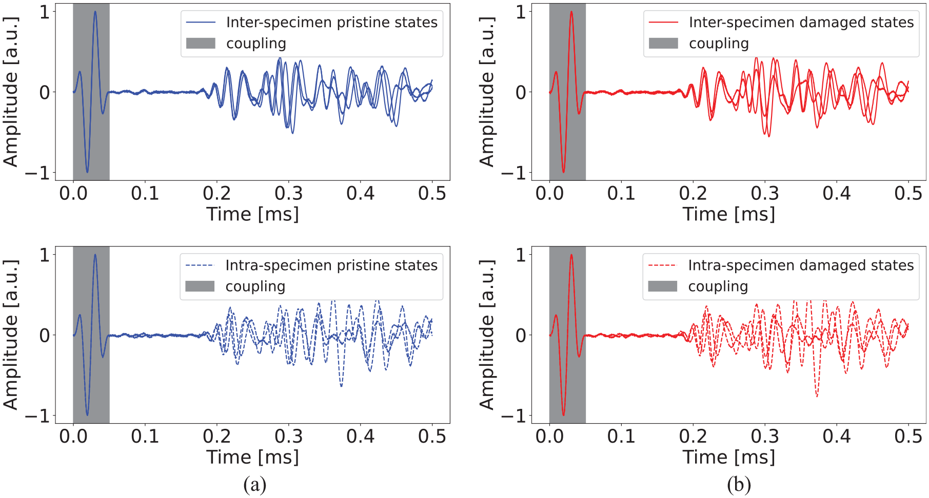
(a) Inter-specimen variabilities: normalized signals corresponding to path 1–4 of three instrumented pristine panels and intra-specimen variabilities: normalized signals corresponding to three paths (similar paths) of one pristine panel, that is, 1–4, 2–5, and 3–6; (b) effect of inter (top) and intra-specimen (bottom) variabilities in damaged case (considering similar paths as in pristine case).
List of intra-specimen and inter-specimen variabilities.
Damage path identification
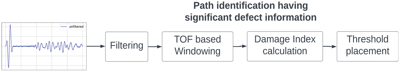
In a pitch-catch measurement method and for a specific defect location, the amount of defect-related information contained by all the paths differs. When the defect is at the center, as shown in Figure 1, not all the paths carry defect information provided windowing based on the arrival of A0 mode. In other words, the adjacent paths (1–2, 2–3, 3–4, 4–5, and 5–6) may carry minimal defect information. Hence, the paths containing significant defect information need to be separated from those not containing. This procedure works as a preprocessing stage in a ML-based classification pipeline. Furthermore, this step is essential to appropriately annotate the data required for supervised ML algorithms. The following steps describe the procedure involved in the signal separation process.
Signal treatment and data annotation
Filtering
In the path identification process pristine and defect signals are compared. Therefore to better learn the effect of a defect, both signals are filtered with a fifth order Butterworth filter allowing frequencies between 20 kHz and
ToF-based windowing
Signal windowing helps remove the reflections depending on the length of the window. The length of a window is decided based on the ToF. It is calculated based on the velocity of the GW-mode, and the path traveled. The velocity of GW-modes is determined from dispersion diagrams. In an anisotropic medium the GW-modes propagate with varying velocities as a function of propagation angle. But for the CFRP panel used in this study they exhibit minimal variation in the group velocities, which is shown in Figure 3(a). Therefore, an average of the velocities is computed (see Figure 3(b)) and used to estimate the ToF.
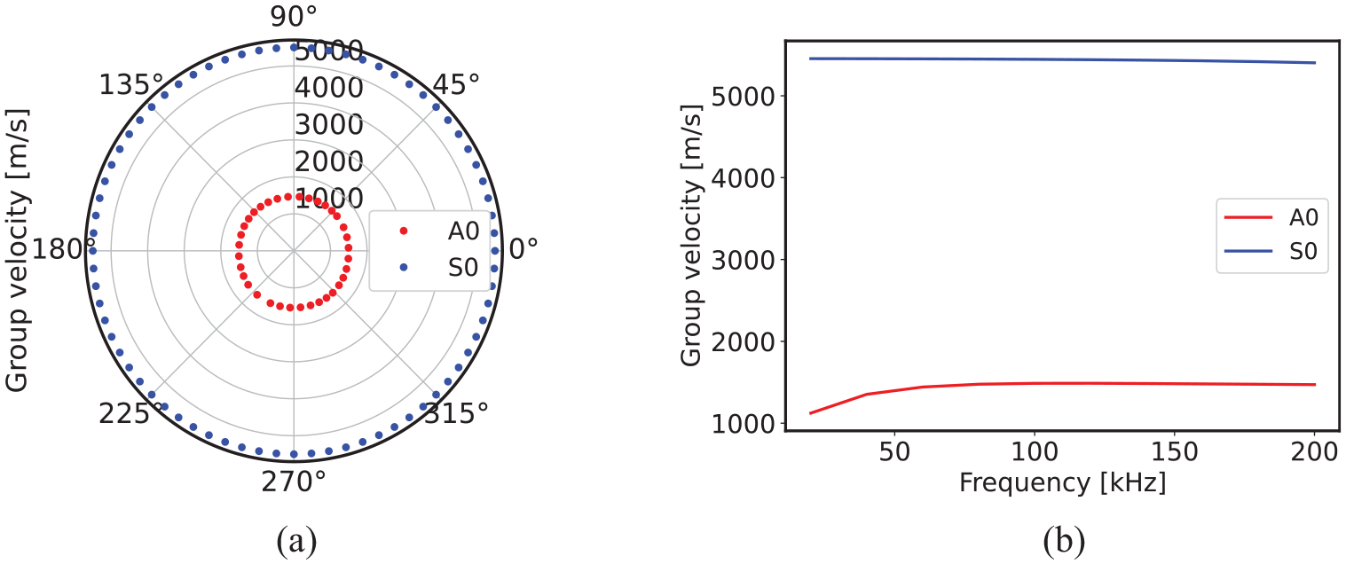
(a) Polar dispersion diagram containing A0 and S0 group velocities at different propagation angles and (b) the averaged group velocity diagram containing average A0 and S0 group velocity.
For the considered frequencies A0 mode is more sensitive to the defect sizes present in the dataset than S0 mode; therefore A0 mode is used for damage detection process. The ToF of A0 mode is computed by a simple velocity, distance, and time relationship which is given below,
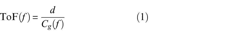
where,
Since the CFRP panel used in the study exhibits negligible changes in the group velocities at different directions, a representative velocity is considered by taking an average of all the velocities. In the case of strong anisotropy, the representative velocity needs to be replaced by individual directional group velocities to extract the ToF information.
Damage index
To quantify significant defect carrying signals, root mean squared deviation (RMSD) as a damage index (DI) is employed. It accounts for the overall changes in a signal by comparing it with a defect-free signal. The mathematical expression of RMSD is shown in Equation (2),
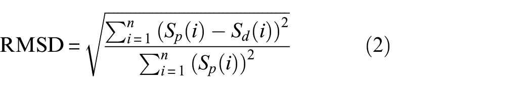
where,
Threshold selection
For supervised ML algorithms, appropriate data annotation is a crucial step. Therefore, appropriate annotation of the signals is accomplished based on the DI obtained for each path in a damaged panel. Not all the paths might carry significant defect information for a specific delamination location in a panel. Referring to Figure 1, where the defect is at the center of the panel, considering the TOF corresponding to just the sensor paths (1–2, 2–3, 3–4, 4–5, 5–6), the GWs do not interact with the defect at all by the time they reach the receiver. Figure 4(b) shows calculated RMSD versus 15 unique paths for defect at the center. Higher DIs correspond to the direct paths, and for defects away from the sensor paths, DI decreases. Similar phenomena is observed for other two defect locations which is shown in Figure 4(a) and 4(c). A threshold is applied to facilitate the separation of higher DI from lower ones. The selection of this threshold is a tricky task and is arbitrary in a way. A higher threshold aiming at picking just very high DIs would lead to data scarcity, which is not desirable, as enough data is required to train ML classifiers. Hence, as a trade-off, a threshold of 0.1 is selected to allow sufficient data in the defect category.
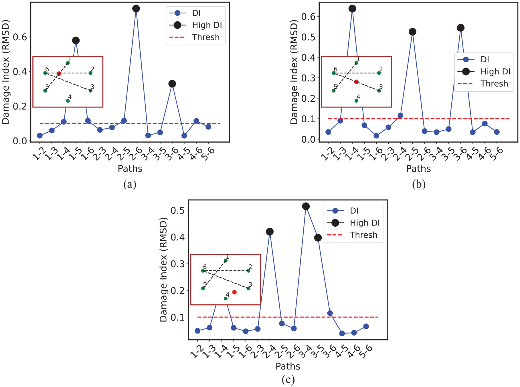
Defect configuration with delaminations at (a) (250, 135) mm, (b) (200, 200) mm, and (c) (150, 300) mm, and their corresponding damage index plots.
Baseline aggregation
In developing an automatic damage detection system for similar structures, the idea is to use a few damaged and a few pristine structures (aggregated baselines). Using aggregated baselines to train the models ensures the coverage of the variability and ensures monitoring of new similar structures even without the availability of baselines. Forty-five panels are divided into two groups to work on this idea. Pristine signals are considered from the group 1 and defect signals from group 2 (see Table 2). The latter group consists of damage-annotated signals resulting from the path identification process. This intermediary step ensures that the baseline signals of the damaged panels are not present in the data set (Figure 5).
Details of data set preparation.
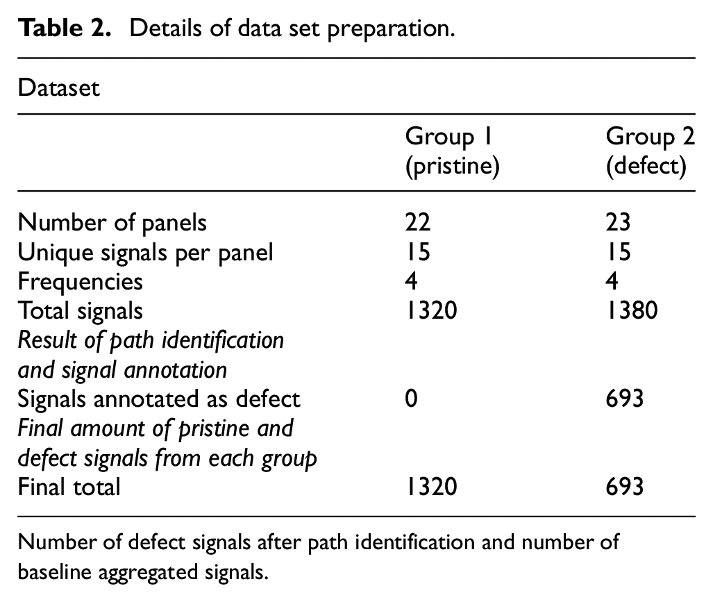
Number of defect signals after path identification and number of baseline aggregated signals.
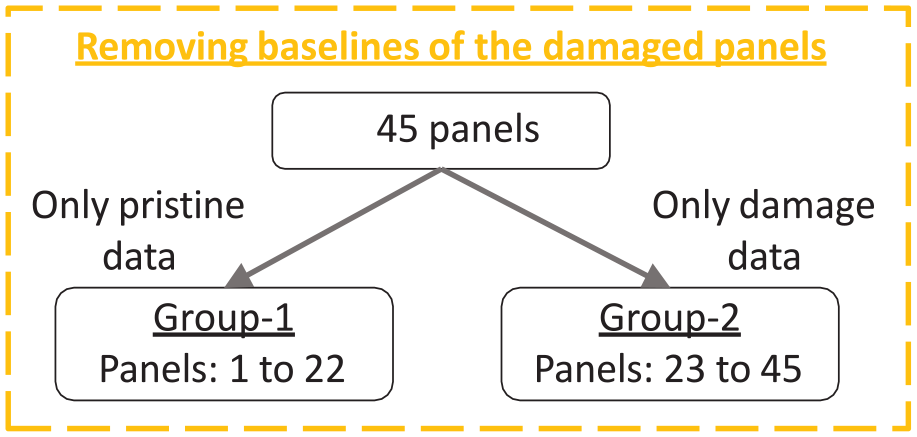
Schematic describing removing baselines of the damaged states. This step ensures that the pristine and damage acquisitions correspond to distinct panels.
A quantification of the pristine and damaged-state signals at the end of data annotation process is presented in Table 2. From here on pristine annotated signals are referred to group 1 signals only and defect annotated signals to group 2.
Feature extraction
The effect of delamination on the GW signals is masked by the presence of inter- and intra-specimen variabilities. Therefore, instead of compensating the effect of the aforementioned variabilities, a feature extraction method is required to extract the defect signatures hidden under the influence of variabilities. Some of the feature extraction methods applied on GW signals include: principal component analysis for extracting features from post processed GW signals 18 and various feature extraction methods, such as principal components and best Fourier coefficients as presented in the study by Schnur et al. 20 The aforementioned feature extraction methods have been shown effective on baseline-corrected signals. But this work aims not to use classical baseline correction methods but instead apply a feature extraction method to extract features hidden under the influence of variabilities. Therefore, AR modeling is employed in this study to extract the hidden defect signatures from raw time domain signals.
AR is a linear combination of immediate preceding values in a sequence. 25 In other words, when a time series is stationary, then modeling the time series on past values yield the current value. A pth order AR model can be represented mathematically as shown in Equation (3).
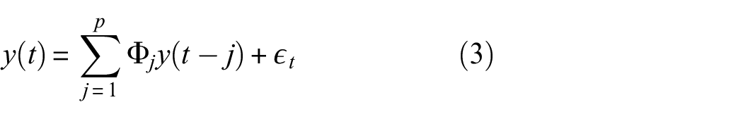
where,
Selection of AR model order is a delicate task, because, higher model orders tend to show poor generalization and lower model orders may not capture the underlying dynamics of the system.
27
Therefore, model order

Where
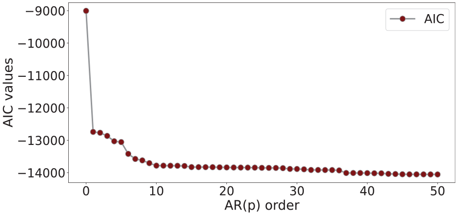
AR model order selection using AIC.
On each windowed raw signal AR model of order 40 is fitted, and the result is 40 encodings (AR model parameters) per signal; the final feature matrix of size
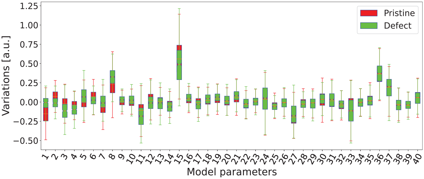
Box plot of reordered AR parameters in the decreasing order of the difference between the means of pristine and defect distributions.
The first ten reordered pristine and defect feature distributions have less overlap than the rest, meaning that the AR model is sensitive to damage information in the presence of the variabilities. This discrimination between pristine and defect feature distributions may be exploited using ML algorithms.
Background of classification algorithms
In SHM, ML algorithms have been used for damage detection and quantification tasks. Some of the established ML algorithms in SHM are listed as follows: Naive Bayes (NB) and kernel-based classifiers, 18 ensemble methods: random forest (RF) classifier 29 and extreme gradient boosting, 30 and convolutional NN. 21 Five different established classifiers from different families of algorithms are chosen to learn the AR encodings. The NB classifier, however, is used as a reference classifier to compare the performance with others. The description of the chosen classifiers is presented below.
NB classifier
NB classifier is based on the Bayes theorem. Consider a random vector (
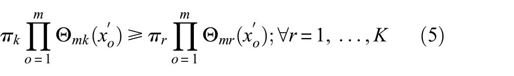
According to the Bayes decision theory, a new observation
Support vector machines
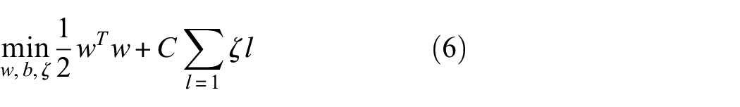
Support vector machines (SVM) algorithm constructs a hyperplane on the training data to separate two classes. Two parallel lines on both sides of a hyperplane exist, called the width/slab. SVM tries to maximize this width, and if this maximum width has no internal training samples, then the hyperplane is said to be best, and the samples lying on the margin are called support vectors.
32
For a linearly separable data, the best hyperplane can be represented by
Dual problem of the soft margin is formulated for easier computations using Lagrange multiplier
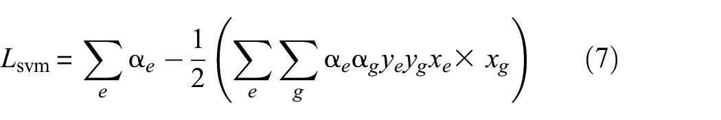
The optimization depends on the dot product of pair of training samples
Random forest
RF is an improvement to the bagging technique, which averages the big collection of de-correlated trees.
34
In other words, averaging over correlated samples does not yield any new information. Therefore training samples are randomly sampled to obtain de-correlated decision trees.
35
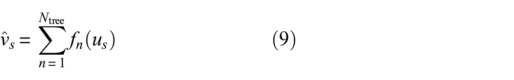
It consists of numerous decision trees. Each of the trees gets independent and randomly sampled samples with the same distribution from the pool of data, and the decision made by this individual classifier is taken into account. The prediction of the RF classifier is the majority vote of the prediction of individual trees. The classification result of the new sample
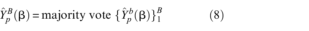
Where
eXtreme gradient boosting
eXtreme gradient boosting (XGB) is a tree boosting-based algorithm proposed by Chen et al.
36
Boosting of decision trees works in a sequential way; in other words, underperforming trees are given more importance so that the outcome is the total response of both boosted trees and learning trees. Weight is added to the weak learners until their performance is better than a random classifier. It has an inbuilt regularization term which helps in reducing overfitting problem and parallel processing enables faster tree building and solving process. Gradient boosting classification of
where,
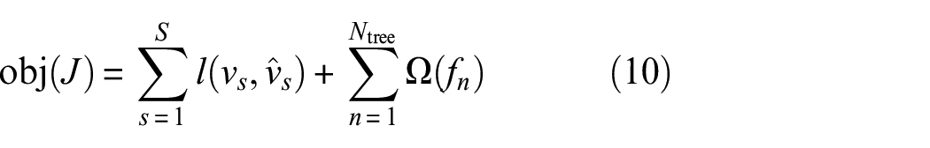
with
Neural network
The simplest form of a NN is a multi-layer perceptron (MLP) and the architecture consists of hidden layers, an input layer, and an output layer. Input layer is made up of input units, output layer is made up of output units and the hidden layers contain the output units of the previous layer, and all these layers are connected by weights.
37
The working of a MLP can be divided into forward pass and backward pass. In the forward pass, the weighted input is passed through an activation function
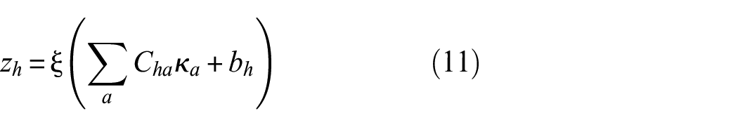
Where,

The error between the predicted label and the ground truth is minimized by re-calibrating the weights in the backward pass. The gradients of weights and bias (

This process continues until the error is reduced significantly. Detailed information about working of NNs and other NN types can be found in.38,39
Hyperparameter space selection
In this study, a range of values is assigned to each of the hyperparameter given a classifier. The best hyperparameter space (i.e., best model) for shallow classifiers is automatically selected through grid search cross validation (CV) 40 strategy with stratified group CV (Appendix B). KerasTuner, a hyperparameter optimization framework with Bayesian Optimization algorithm, 41 is employed to select the best hyperparameter space for MLP. Defining the range of hyperparameter values is a crucial step and it is defined based on the recommendations in the study by Pedregosa et al. 40 First a large range of coarse values was used to get an intuition of the range required to tune the models. The range of hyperparameter values are mentioned below.
Support vector machines
There are three main parameters to be chosen carefully: (1) the type of kernel function; (2)
Random forest
List of hyperparameters chosen to be tuned. (1) The number of trees:
eXtreme gradient boosting
In XGB there are four categories of parameters, namely: General parameters, Booster parameters, Learning task parameters, and Command line parameters. The tunable parameters are (1) The number of trees:
Multi-layer perceptron
Some of the parameters used for tuning: (1) Adam optimizer with learning rate sampled from
Performance evaluation and reliability assessment
The performance of ML models is evaluated using performance measures; their selection depends on the main objective of the evaluation. They can broadly be categorized into three groups as listed in the study by Ferri et al. 42
Threshold-based measures: These measures are used when the total prediction error is to be minimized. Examples include accuracy, F-score, Kappa statistic, and so on. Some of the measures are suitable for balanced and/or imbalanced data sets.
Probabilistic measures: These measures quantify the uncertainty in the predictions and are useful to assess the reliability of a classifier. Some examples include cross-entropy and Brier score.
Rank-based measures: They do not focus on minimizing prediction errors based on the quality of one particular choice of threshold; rather, they measure the class separability of a classifier at different thresholds. Receiver operating characteristic (ROC) curve, precision-recall (PR) curve, and area under these curves fall in this category.
In the SHM domain, the damaged case is labeled as a positive instance and the undamaged case as a negative instance. The false positives (damage indication when it is not present) incur downtime, which causes revenue loss and results in a less reliable SHM system. Whereas, for misclassifications, false negatives (no damage indication even though it is present) means the risk of human life (in the case of rail and aircraft applications) is at stake. Furthermore, it is desirable to have trade-offs between false positives and false negatives, that is, when an SHM application is focused more on costs than life-safety, false positives need to be minimized (false positive is given more emphasis than false negative). On the other hand, if life safety is of paramount importance, then false negatives need to be minimized (false negative is given more emphasis than false positive). 43 Especially in aircraft applications, a trade-off between false positives and false negatives is desired. Therefore, a performance measure providing this trade-off becomes essential.
One more commonly encountered problem in a SHM system is that, undamaged instances usually outnumber damaged ones because the continuous acquisition of sensor data comes from a healthy condition and damage episode seldom occurs. Consequently, there is a natural imbalance in the data, and in such scenarios, not all measures are effective. In such cases, measures, which are less sensitive to class skew are appropriate. Rank-based measures are not sensitive to class skew, whereas threshold-based measures are sensitive to class skew. Hence, the ability of a classifier to separate a positive class from a negative class does not suffer while using rank-based measures. 44
The trade-off between false positives and false negatives can be obtained by plotting a ROC curve. It is a graphical representation of false positive rate versus true positive rate; each point on the ROC curve corresponds to a unique threshold. It gives an excellent visual of the behavior of a classifier on a given data-set, and a trade-off between false positives and false negatives. A single quantity of measure derived from the ROC curve is area under the curve (AUC), which is used in addition to provide more clarity. 45 The PR curve is one more measure that does not provide very optimistic results like ROC in the case of data imbalance because it focuses more on the minority class. 46 In this study, the AUC of ROC curves is used to measure the performance of classifiers on balanced data and the AUC of PR curves for imbalanced data; from here on we refer to them as ROC_AUC and PR_AUC respectively.
The probability of detection assesses the reliability of a monitoring system which is widely being used in the NDT community. It’s a fundamental evaluation technique that informs as to what size of defect the system can detect with 95% confidence. Usually, the critical defect size is supposed to be less than
Experimental validation
Parametric study to select AR features
As shown in Figure 7, 40 AR parameters are extracted from pristine and damage signals. From here on, AR parameters and features are used interchangeably. To determine how many of those 40 parameters are necessary to obtain the best performance, a parametric study is conducted by varying the AR parameters and training samples. Note that the parametric study’s primary focus is selecting the optimal number of features, not the number of training samples. The left side flowchart as shown in Figure 8 presents the parametric study methodology, wherein the first stage forms groups of aggregated baselines and damage signals, then features are extracted through AR modeling of group 1 and group 2 signals.
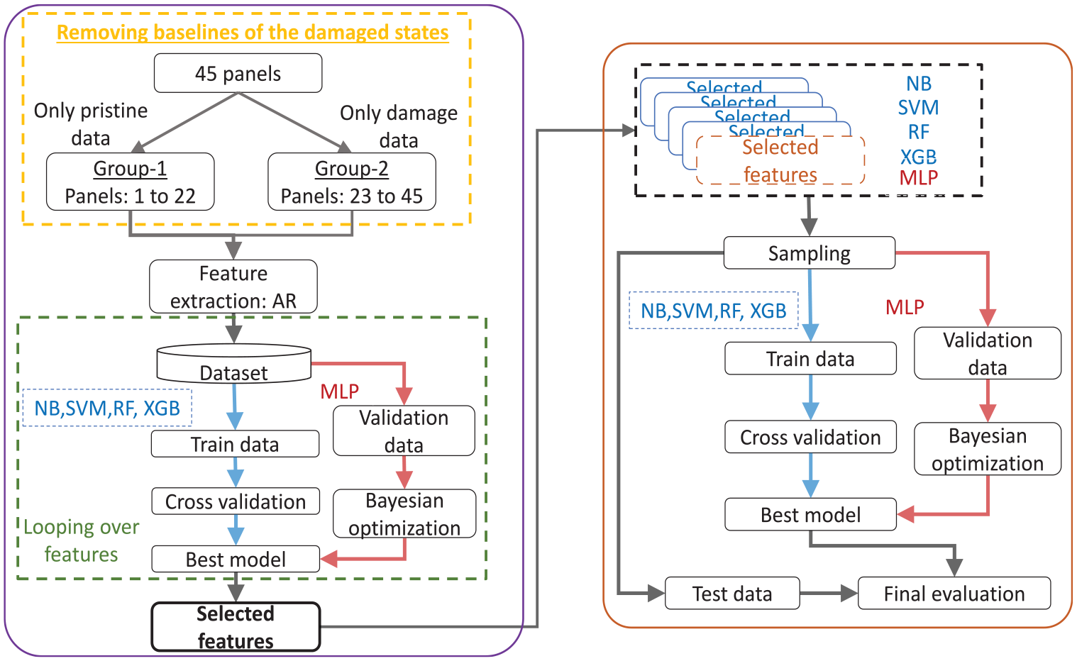
The left side flowchart shows the feature selection schema starting from feature extraction applied on grouped classes, followed by hyperparameter space optimization algorithms to determine the required features. The right-side flowchart shows the final training and evaluation procedures, starting from considering selected features from the feature selection schema. The best shallow and MLP models are obtained by grid search CV and KerasTuner with Bayesian Optimization algorithm, respectively.
A feature set containing six varying features starting from four with step six in increasing order is formed. Similarly, a training sample set is formed with five varying training sample sizes. These two formed sets result in a total of 30 combinations of features and training sample sizes. For each of the 30 combinations, the best hyperparameter space (i.e., best model) for shallow classifiers is automatically selected through grid search CV with stratified group CV (the CV groups formed are equivalent to the number of CFRP panels to enable the models to train on signals from some panels and validate on an entirely different set of panels) and for MLP KerasTuner with Bayesian Optimization algorithm is employed. For each of the 30 combinations and for each of the classifiers, the mean of the CV scores based on ROC_AUC is plotted as shown in Figure 9. The X-axis shows the increasing volume of training samples, Y-axis shows the increasing number of features, and the Z-axis presents the validation results (i.e., ROC_AUC score).
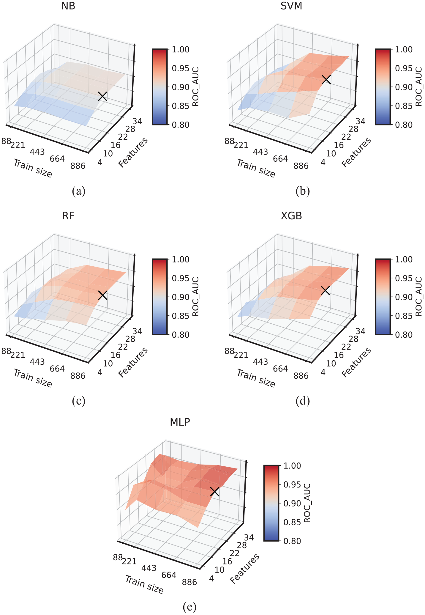
Surface plots representing the learning of classifiers as a function of features and training samples of (a) Naive Bayes, (b) support vector classifier, (c) RF, (d) XGB, and (e) MLP. The X-axis shows size of the train set, Y-axis shows number of features, and Z-axis shows the mean ROC_AUC score. The cross markers (×) on each of the plots indicate the selection of necessary features resulting in best performing models; the necessary features selected are 16.
All the plots correspond to each of the classifiers in Figure 9 exhibit increasing ROC_AUC scores with the increasing number of features and training samples. This increment can be tracked by the elevation of the plots and dark red color shades, which correspond to higher ROC_AUC. The minimum number of required features is selected based on the best-performing model given the combination of features and training samples. All classifiers’ best models are obtained at 16 features, and the cross marker (×) indicates this selection on the plots. Therefore, for the final training and evaluation of the classifiers, the selected 16 features are used.
Model training and evaluation with uncertainty assessment
The final training set used for training the five classifiers can be represented as
Process used for performing data annotation.
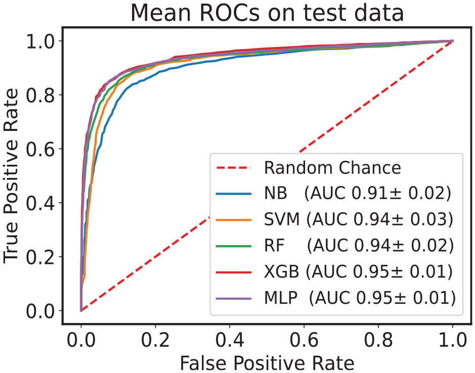
Mean ROC curves and AUC with standard deviation computed on balanced test data set.
A classifier is said to have the best performance when the point in the ROC curve is bowing toward the top left corner. Comparing performances of multiple classifiers based on the ROC curve is cumbersome. Therefore, a single scalar measure, AUC, is often used as a performance metric. In Figure 11, the AUCs are shown with corresponding deviation due to 25 models. All the classifiers registered more than
The mean train and test ROC_AUC scores and the variance of the predicted results for the balanced data set.
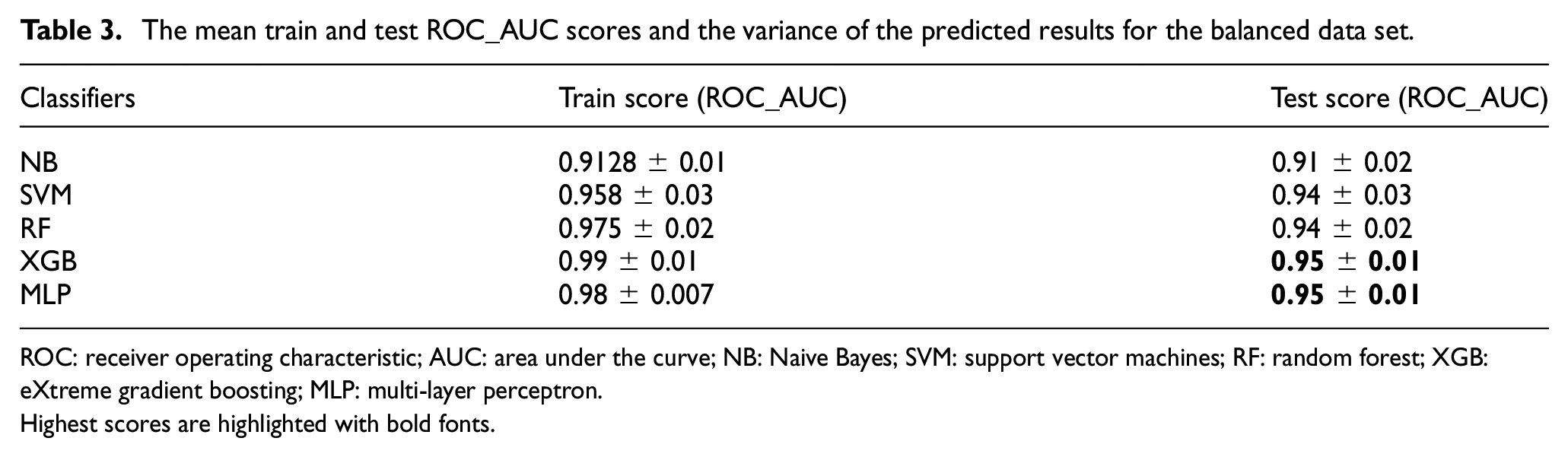
ROC: receiver operating characteristic; AUC: area under the curve; NB: Naive Bayes; SVM: support vector machines; RF: random forest; XGB: eXtreme gradient boosting; MLP: multi-layer perceptron.
Highest scores are highlighted with bold fonts.
As discussed in performance evaluation section, the SHM system often results in imbalanced pristine and defect instances. Therefore, a thorough study is conducted to test how close the classifiers’ performance with imbalance gets to that with the balanced case. To this end five imbalanced data sets are prepared (artificially) with varying imbalance ratios (IRs), namely 60–40%, 80–20%, 90–10%, and 95–5% (pristine–damage%). However, train samples and test samples are kept constant for all data sets and is same as for the balanced data set, that is, 886 train samples and 278 test samples. The same methodology is applied for all the considered imbalance cases as shown in Figure 8. However, in the sampling stage, both pristine and damage samples are randomly sampled with replacement. The mean of the CV score, that is, PR_AUC is presented in Figure 12 with error bars representing the variance. The best set of hyperparameters corresponding to the first among the 25 models are presented in Appendix A, Table A1. The plot contains the mean test scores of all the classifiers. The PR_AUC is along the Y-axis and the ratio of pristine samples is along the X-axis. Some of the observations are listed below,
With increasing IR:
– The mean scores of all the classifiers decrease gradually.
– The variance of the test scores increased, but the variance of RF and XGB is lower compared to others.
The best performance is observed when the data set is balanced and is worst for strong IR.
At 60% IR and 50% pristine ratio, no significant change in the performance is observed. But for further reduction in the minority class ratio, the performance starts decreasing significantly.
NB exhibited the lowest mean score for balanced case and the rest of the classifiers showed higher mean scores.
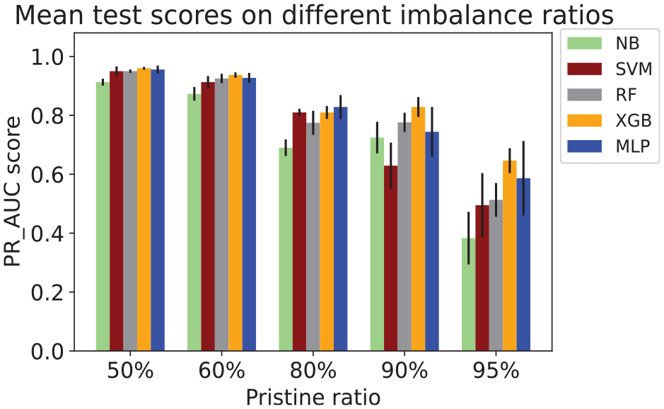
Mean test precision-recall AUC with variance depicted in error bars for all the IR and classifiers resulting from 25 models.
Creating imbalances reduces representative samples of the minority class, which makes it difficult for the classification algorithms to learn to distinguish from the majority class. The experimental data used here needs to be larger; therefore, creating an imbalance further reduces the representative samples from an already small-sized data set. Hence, degradation in the classifiers’ performance is observed with increasing imbalance.
POD analysis
Following the classification of GW signals, the next step involves analyzing the classification results using probability of detection to identify what defect sizes are being correctly detected. The data set contains signals corresponding to 4 frequencies and the defect size varies from 14 to 27.5 mm. Hit/Miss algorithm is employed on the predicted defect classes to compute the probability of detection curve. Since the trend in the plots obtained from all the classifiers’ predictions is similar, just one plot obtained from SVM is presented in Figure 13. Along the X-axis are the defect sizes and % probability of detection along Y-axis. The trend observed in the plot suggests that, larger defects are identified accurately which is a good indication for the damage detection system.
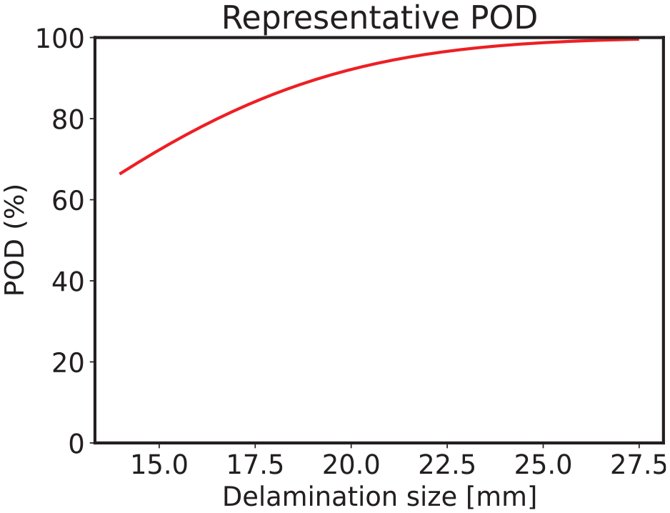
POD computed on the model predictions represented by the red curve. The POD curve shown here is the representative result of PODs obtained from all five classifiers’ predictions.
Discussion
In the previous sections, we showed the challenges in damage detection due to intra- and inter-specimen variability by considering the measurements acquired on 45 CFRP panels. We performed the analysis by considering variability inclusion and baseline aggregation. Furthermore, an AR-based feature extraction method is applied to avoid using baseline correction methods, and classifiers are used for the detection task. The results obtained show an excellent classification performance of 95% (ROC_AUC) and show the robustness of the approach to intra- and inter-specimen viability. The data set presented in the previous section contains a minor variation in the temperature. Therefore, an alternative data set is considered to investigate the effect of the temperature (i.e., OpenGW 22 ), and the same methodology is applied to it.
Impact of temperature variation:a preliminary study
The GW signals measured on CFRP panels with real-impact-caused delaminations were analyzed in the previous data set. Unfortunately, the experiment campaign was carried out in a laboratory setup with minor temperature variations. On the other hand, it is well known that temperature variation can significantly influence GW propagation in both isotropic and anisotropic materials. Therefore, to provide a preliminary validation of our proposed methodology in the presence of high-temperature variation, we decided to consider the OpenGW 22 data set, which contains measurements performed on CFRP with temperature variation between 20 and 60°C. It is also worth mentioning that the instrumentation and artificial defect (mass attachment) makes this problem more academic than the previous one (brief details about the OpenGW data set are given below). Nevertheless, we believe the proposed methodology can directly be applied to this data set to assess the robustness of baseline aggregation and AR-based feature extraction under significant temperature variations.
The measurements are conducted on a composite plate instrumented with 12 piezoelectric transducers, and reversible damage is placed by attaching weights on different locations (see Figure 14). For a detailed explanation of the experimental setup and acquisition, the readers can refer to this article.
22
The study is conducted by forming four groups with increasing temperature variations, that is,
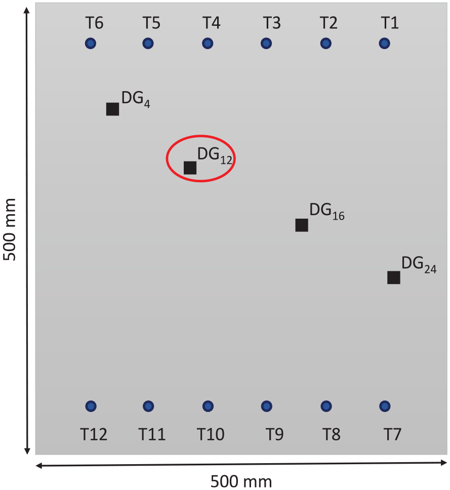
CFRP plate instrumented with 12 PZTs and a reversible damage placed at either 4 locations to acquire measurements.
The path identification schema is employed with the same threshold (i.e., 0.1) as used in the former data set to identify more defect information-carrying paths (see Figure 10). All the identified paths carrying more damage information are grouped under the damage class, and all the aggregated baselines are grouped under the pristine class. AR modeling is applied to both groups to extract the features. Five classifiers are chosen to learn to distinguish the feature space: NB, SVM, RF, XGB, and MLP. Measurements corresponding to just one excitation frequency (i.e., 40 kHz) are considered to conduct the preliminary study. However, except for the CV strategy, the same feature selection and final training methodology are applied as shown in Figure 8. Features selected (η) for all temperature groups are
The mean train and test ROC_AUC scores for varying temperature ranges.
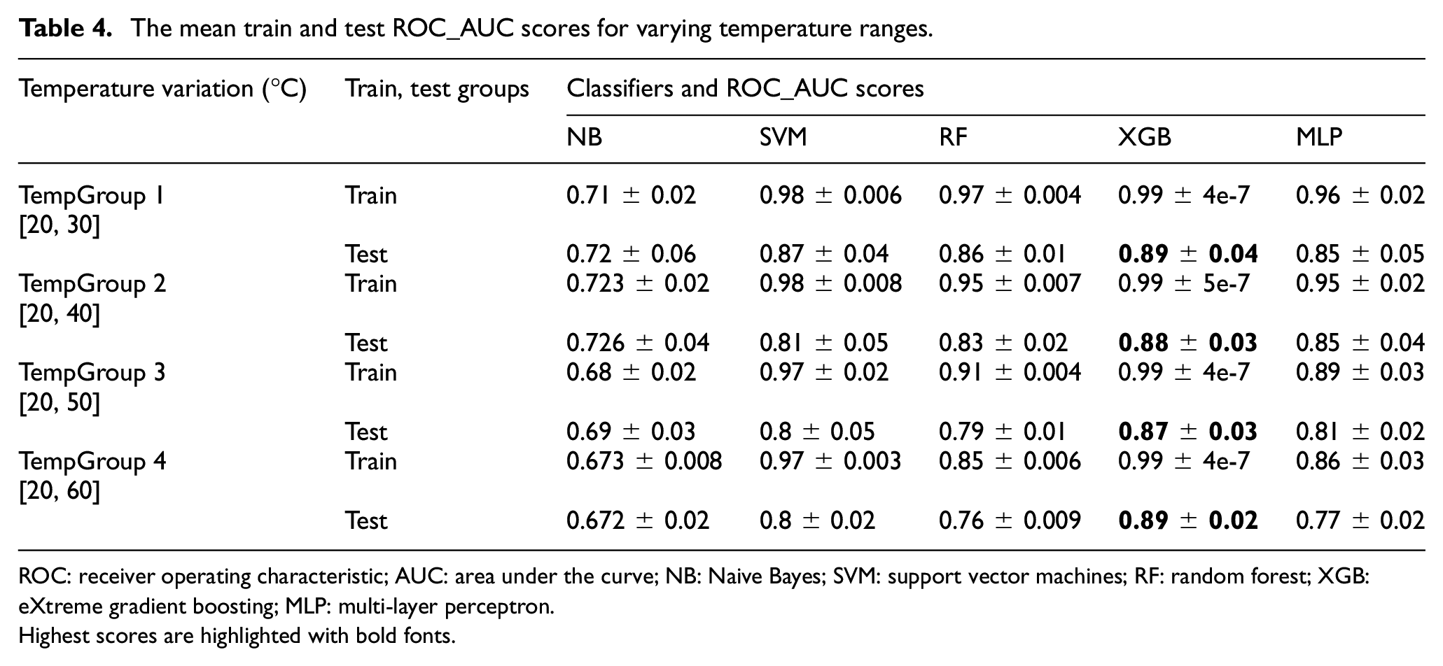
ROC: receiver operating characteristic; AUC: area under the curve; NB: Naive Bayes; SVM: support vector machines; RF: random forest; XGB: eXtreme gradient boosting; MLP: multi-layer perceptron.
Highest scores are highlighted with bold fonts.
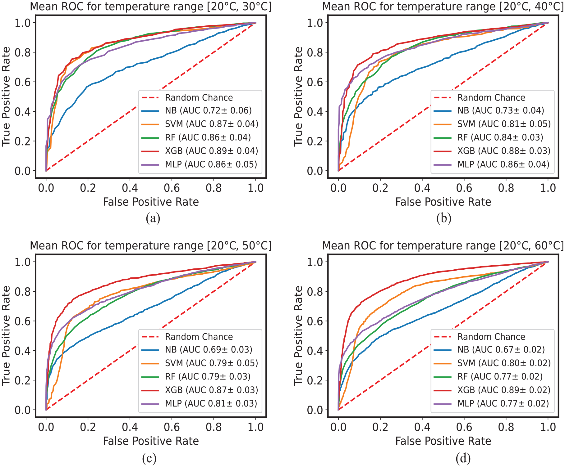
Mean ROC curves with AUC values computed on the test set for temperature variations (a)
Comparison to the state-of-the-art and discussion
These results obtained can be considered promising when compared with very recent works on the same data set20,23 mentioned in the introduction. Schnur et al. 20 performed classification by compensating the temperature effect through optimal baseline selection and baseline signal stretch methods. Furthermore, the authors analyzed just two sensor pairs, that is, T4→T9 and T1→T7, to apply compensation methods and classification schema. With the best Fourier coefficients (features) and SVM, they showed high classification accuracy with temperature compensation. In another work, Abbassi et al. 23 compared four unsupervised dimensionality reduction algorithms to obtain latent vectors and used them for damage detection. They showed high detection accuracies on four temperature groups formed between 20 and 60°C with 10°C step.
On the other hand, comparing our proposed methodology with the study by Schnur et al.
20
has shown to be very effective under more considerable temperature variations without the need for temperature compensation and aggregating various sensor pairs (i.e., baseline aggregation). Furthermore, comparison with the study by Abbassi et al.
23
shows that the proposed methodology works for shorter and wider temperature ranges, that is,
The FPR in a GW-SHM system is generally expected to be relatively low (i.e., less than a few percent). However, depending on the application and the system, the actual FPR can vary. The results obtained with the proposed methodology suggest that the methodology is robust to substantial temperature variations. Nevertheless, the mean AUC_ROC and, in turn, the FPR shown in Figure 15 can be further improved by enhancing the data set.
Conclusions and perspective
In GW-SHM, intra- and inter-specimen variabilities have significant impact on the reliability of detection systems. A methodology is proposed containing variability inclusion and baseline aggregation. With AR-based features and classifiers, the final classification results show that classifiers can distinguish the two classes and have the highest classification performance of 95% ROC_AUC by XGB and MLP. The results suggest that the methodology is robust to variabilities such as instrumentation, material properties, damage size, and location.
To study the impact of significant temperature variations (absent in the former data set), we consider an alternative data set based on GW measurements on CFRP (i.e., OpenGW data set). The same proposed methodology is applied to this data set. For increasing temperature variations, an average of 5% drop in the performance of the classifiers is observed, except for XGB, which registered only a 2% drop; furthermore, for all the temperature variations, XGB exhibited an average of 89% ROC_AUC, suggesting that it is the more robust and stable classifier to large temperature variations. Furthermore, XGB classifier has shown to be the most robust classifier on both the data sets (i.e., inter-specimen variability and large temperature variations).
Our future research will focus on the performance of the robustness of classification algorithms based on GW signals under the influence of intra- and inter-specimen and temperature variability. Toward this end, simulations can add synthetic data to the measurements as a data augmentation procedure based on physics.
Footnotes
Appendix A
Appendix B
Acknowledgements
The authors would like to thank Dr Arnaud Recoquillay for providing valuable suggestions and advices particularly during the revision phase.
Author contributions
VN was involved in conceptualization, formal analysis, methodology, software, wrote—original draft, wrote—review and editing. OM was involved in conceptualization and supervision. RM was involved in conceptualization, supervision, methodology and wrote—review and editing. OD was involved in project administration, funding acquisition, and resources.
Declaration of conflicting interests
The author(s) declared no potential conflicts of interest with respect to the research, authorship, and/or publication of this article.
Funding
The author(s) disclosed receipt of the following financial support for the research, authorship, and/or publication of this article: This work was supported by the European Union’s Horizon 2020 research and innovation program under the Marie Sklodowska-Curie grant agreement [grant number: 860104].