Sage Journals: Discover world-class research

Abstract

To accurately diagnose the quayside container crane (QCC) gearbox faults, this article proposes a method that combines the frequency-domain Markov transformation field (FDMTF) and multi-branch residual convolutional neural network (MBRCNN). Firstly, the gearbox vibration signal is converted into the frequency domain to reveal the components and amplitude of signals stably and concisely. Then, the one-dimensional frequency signal is encoded into the two-dimensional image by the Markov transformation field to capture the dynamic characteristics of signals. Thirdly, the MBRCNN network is constructed, which can extract multi-scale features and alleviate the problems caused by the deep network structure. Finally, the FDMTF image is fed into the constructed MBRCNN model for pattern recognition. The effectiveness of the proposed FDMTF–MBRCNN method is verified by two case studies. In Case 1, the diagnosis results of a benchmark dataset achieve 100% accuracy, better than seven state-of-the-art methods published in recent 3 years. In Case 2, the diagnosis results of the dataset collected from a 1:4 scaled test rig achieve 98.85% accuracy, better than eleven encoding methods and four convolutional neural network methods. It also can obtain a recognition accuracy of more than 94% under the conditions of small sample, different network hyper-parameters, or variable loads, which verifies its robustness. These case studies show that the FDMTF–MBRCNN method is expected to be applied to the actual fault diagnosis of QCC gearboxes.

Keywords

Fault diagnosis frequency-domain Markov transformation field multi-branch residual convolutional neural network small sample variable load

Introduction

Due to the unique advantages of stable transmission performance and high transmission efficiency, gearboxes are widely used in key transmission systems of various machinery, such as wind turbines automobile sectors, machining machines, robots, quayside container cranes (QCCs), etc.^1–3 As the key mechanical equipment of cargo transportation ports, the QCC is specially used for loading and unloading.² The QCC is located in a harsh working environment, which increases the failure rate of gearboxes that bears a huge dynamic load for a long time. Typical common gear faults include gear wear, tooth root crack, gear fatigue and tooth breaking.¹ These gear faults as well as bearing faults will cause damage to the transmission system and easily induce other faults.^1,3 In addition to the increase in operation and maintenance costs, gearbox faults also lead to a catastrophe for the machine, resulting in huge economic losses.⁴ Fault diagnosis can improve the reliability and safety of machinery and reduce operation and maintenance costs.^5,6

Due to rapid response and no need for too much professional knowledge, the intelligent fault diagnosis method has received extensive attention.⁷ According to the depth of the model, intelligent fault diagnosis methods can be roughly classified as machine learning model-based and deep learning model-based. The machine learning-based fault diagnosis methods roughly include three steps: manual feature extraction, dimension reduction and classification model construction. Commonly used features include time-domain features, frequency-domain (FD) features and time–frequency features. Feature selection is a feature dimensionality reduction method, which removes redundant information by selecting feature subsets, to accurately distinguish multiple categories of health and fault states.⁸ There are many shallow machine learning models for classification, such as support vector machine,⁹ extreme learning machine,¹⁰ K-nearest neighbor,¹¹ etc. On the one hand, manual feature extraction depends on prior knowledge, and its universality is poor.¹² On the other hand, it is difficult for machine learning models to express complex mapping.¹³

Compared with machine learning, deep learning models integrate adaptive feature extraction as well as classification and can represent/learn complex nonlinear mapping.¹⁴ Deep learning models, such as deep belief network,¹⁵ stacked autoencoder (SAE),¹⁶ recurrent neural network¹⁷ and convolutional neural network (CNN),^14,18–20 have been widely used in mechanical fault diagnosis. Among them, CNN can significantly decrease the number of training parameters, because of its characteristics of local connection, weight sharing and pooling operation.^18,21 Considering that the original intention of CNN is to classify images, CNN is inclined to classify two-dimensional (2D) images.^14,19 Therefore, how to transform the one-dimensional (1D) vibration signals into 2D images is a meaningful topic in fault diagnosis.^19,21 Many signal processing methods have been used to encode 1D vibration signals into 2D images for mechanical fault diagnosis, such as FD transformation, that is, the spectrum,²² short-time Fourier transform (STFT)²³ and continuous wavelet transform (CWT).²⁴ Other methods such as recursive plots (RP),²⁵ Gramian angle field (GAF) that is divided into Gramian angular summation field (GASF) and Gramian angular difference field (GADF),²⁶ and Markov transformation field (MTF)^26,27that can encode time series into 2D images can also be considered for fault diagnosis based on CNN. Hsueh et al.²⁸ converted the 3-phase current signals into images through RP as the input of CNN for rotating machinery fault diagnosis. Tang et al.²⁹ encoded the vibration signal into a GASF image and achieved an accuracy 99% of mechanical fault identification. He et al.³⁰ used MTF to map the 1D monitoring signal into the 2D image, which improves the fault diagnosis accuracy of the nuclear power system. Han et al.³¹ compared the characterization ability of GAF and MTF in bearing fault diagnosis cases and pointed out that MTF retains more dynamic information than GAF. It should be noted that the above methods directly encode 1D vibration signals into 2D images, which may be vulnerable to being disturbed by arbitrary shocks and background noise.

Bai et al.³² pointed out that in addition to characterizing 1D vibration signals, building a good network structure is also important for fault diagnosis. There are many main stream structures of CNN, such as AlexNet,³³ GoogLeNet,³⁴ ResNet,³⁵ etc. used in image recognition. These classical models provide many references for the construction of CNN. For example, the multi-branch (MB) module of GoogLeNet can learn different features. The residual module can alleviate the problems of network degradation and gradient disappearance/explosion. Inspired by GoogLeNet, Wu et al.³⁶ proposed an enhanced multi-scale CNN for high-speed train rolling bearings. Zhang et al.³⁷ constructed an improved ResNet through the hybrid attention mechanism for wind turbine gearbox fault diagnosis. In addition to the network structure, the hyper-parameters in CNN training, such as learning rate, epoch and mini-batch size, also affect the identification accuracy and generalization of the diagnosis model. To obtain a CNN model that is insensitive to hyper-parameters, Zhang et al.¹⁹ proposed an MB module, which can adaptively adjust the branches to adapt to the preset hyper-parameters. The study aims to design multiple networks, which is complex to choose the most appropriate network by using the minimum loss function. In a few words, a CNN model that is insensitive to hyper-parameters is worthy of further exploration.

Two characteristics of the QCC gearbox that need attention. One is that the number size of fault samples is small, and the other is that QCC often works under different loads. These should be considered in verifying the diagnosis methods. To address the above issues, a QCC gearbox fault diagnosis method combing FDMTF and multi-branch residual CNN (MBRCNN) is proposed. Compared with the time-domain signals, the FD signals can more stably and concisely reveal the components and amplitude of signals. The phase of the signal and a random instantaneous impact will change the shape of the time-domain waveform. In the FD, the phase change of the signal will not affect the shape of the spectrum. It is difficult for short shocks in the time domain to show huge amplitude in the frequency. Because the FD reflects all components of the signal, and the frequency amplitude corresponding to an instantaneous impact may be low. The MBRCNN combines MB block and residual block to extract multi-scale features and eliminate a series of problems caused by the deep structure. Our specific contributions and insights are as follows:

A new gearbox fault diagnosis method is proposed for the QCC gearbox, which benefits the FDMTF and MBRCNN. Its performance is explored based on two case studies, including a benchmark gearbox dataset and a dataset collected from a QCC scaled-down test rig. Its robustness is also explored, which lies in handling different proportions of training samples, different hyper-parameters as well as variable loads.

The representation ability of FDMTF for 1D vibration signal is comprehensively studied. Firstly, the representation effect of FDMTF for time series is compared with that of MTF. Secondly, the feasibility of FDMTF for the representation of gearbox vibration signals is explored. Finally, FDMTF is compared with other 2D representation methods, such as GASF, GADF, FDGASF, FDGADF, RP and FDRP, etc. in the case of QCC gearbox fault diagnosis.

A CNN network structure, that is, MBRCNN integrating the MB block and the residual block is proposed, to facilitate extracting the multi-scale features and alleviate the problems caused by deep network layers.

This article is arranged as follows. Section ‘The frequency-domain MTF’ proposes the FD MTF and compares the performance of FDMTF and time-domain MTF. Section ‘The proposed fault diagnosis method’ proposes the gearbox fault diagnosis method for QCC based on FDMDF–MBRCNN. Section ‘Case study’ is the case study based on two datasets. Section ‘Conclusions’ provides some conclusions.

The frequency-domain MTF

Markov transformation field

MTF^26,27 can capture the dynamic characteristics in time and frequency. Given a time series x = {x₁, x₂, …, x_N}, the main process of obtaining MTF is as follows. Firstly, the time series is divided into Q bins (similar to quantiles) according to the values of x_i, and each x_i is mapped to a corresponding interval q_m. Secondly, by calculating the transfer probability between q_m in the way of the first-order Markov chain along each time step, a Markov transition matrix W is constructed with Q × Q.

W = [\begin{matrix} ω_{11} & \dots & ω_{1 Q} \\ ⋮ & ⋱ & ⋮ \\ ω_{Q 1} & \dots & ω_{QQ} \end{matrix}]

(1)

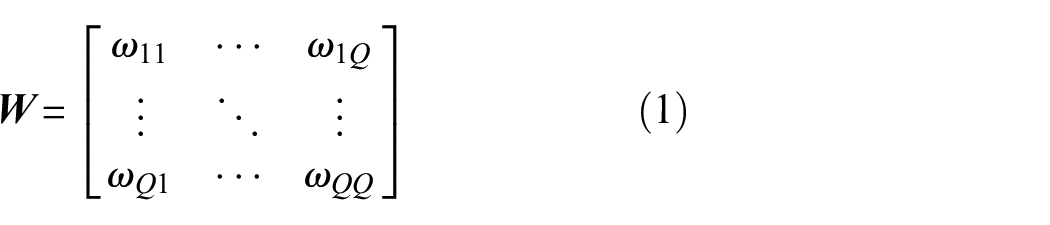
where ω_mn is the probability that an element in q_m is followed by an element in q_n, that is, ω_mn = P(x_t∈q_m|x_t ₋ ₁∈q_n); m, n∈[1, Q].

Finally, the MTF is extended by each probability of the points of the original time series x to generate the MTF M of N × N.

\begin{matrix} M = [\begin{matrix} M_{11} & \dots & M_{1 N} \\ ⋮ & ⋱ & ⋮ \\ M_{N 1} & \dots & M_{NN} \end{matrix}] \\ = [\begin{matrix} ω_{mn | x_{1} \in q_{m,} x_{1} \in q_{n}} & \dots & ω_{mn | x_{1} \in q_{m,} x_{N} \in q_{n}} \\ ⋮ & ⋱ & ⋮ \\ ω_{mn | x_{N} \in q_{m,} x_{1} \in q_{n}} & \dots & ω_{mn | x_{N} \in q_{m,} x_{N} \in q_{n}} \end{matrix}] \end{matrix}

(2)

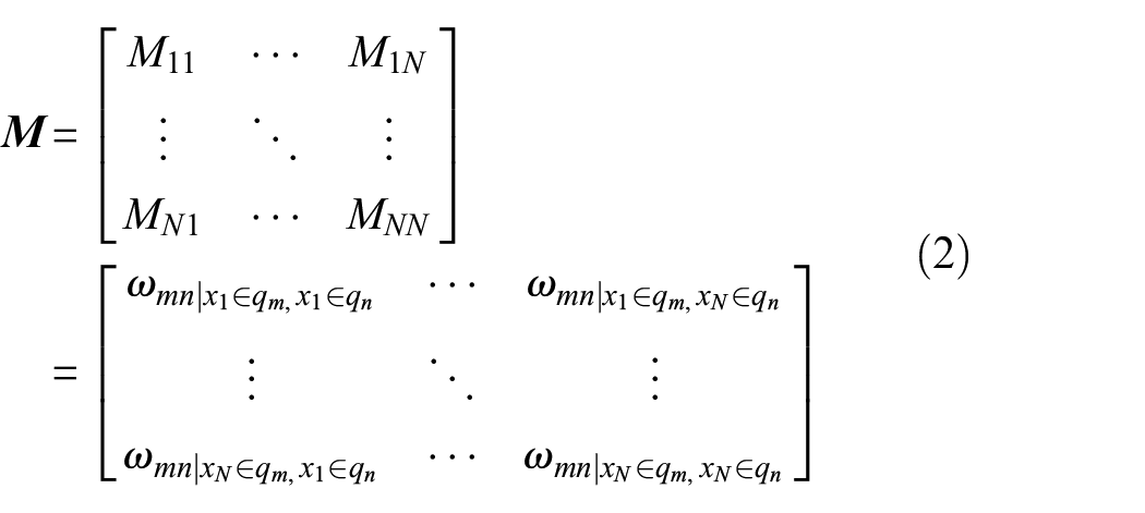
where M_ij(i, j∈{1, 2, …, N}) is the probability that the interval q_m corresponding to time series x_i is transferred to the interval q_n corresponding to time series x_j.

The proposed FDMTF

For the above time series x , the FD series is obtained by discrete Fourier transform, which is expressed as follows:

{\tilde{x}}_{k} = \sum_{i = 0}^{N - 1} x_{i} e^{- j \frac{2 π}{N} i}

(3)

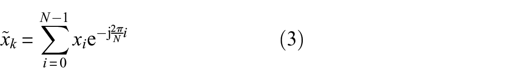
where ${\tilde{x}}_{k}$ is an element of the FD series; k=0, 1, …, N−1.

To obtain the actual FDMTF, it is generally necessary to normalize the FD signal to the interval [−1, 1], and the normalized series is given by:

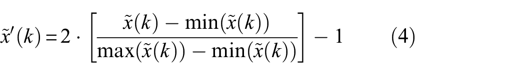
\tilde{x}' (k) = 2 \cdot [\frac{\tilde{x} (k) - min (\tilde{x} (k))}{max (\tilde{x} (k)) - min (\tilde{x} (k))}] - 1

(4)

The FD series of Equation (4) is treated as a sequence to be processed by Equations (1) and (2) to obtain the FDMTF. To prove the advantages of FDMTF over time-domain MTF, we intercept different time intervals of the same signal to compare the encoding ability.

This signal is used to compare the GAF and FDGAF in Bai et al.,³² which can be expressed as follows:

s = 0.7 \sin (2 π \cdot 50 t) + \sin (2 π \cdot 20 t)

(5)

The sampling time is 0.5 s with the sampling frequency = 512 Hz. Figure 1 shows this time signal. Divide the signal into two parts for the characterization of MTF and FDMTF. The black line is the original signal s, the blue line is the first half signal s₁ of s and the red line is the second half signal s₂ of s.

Figure 1.

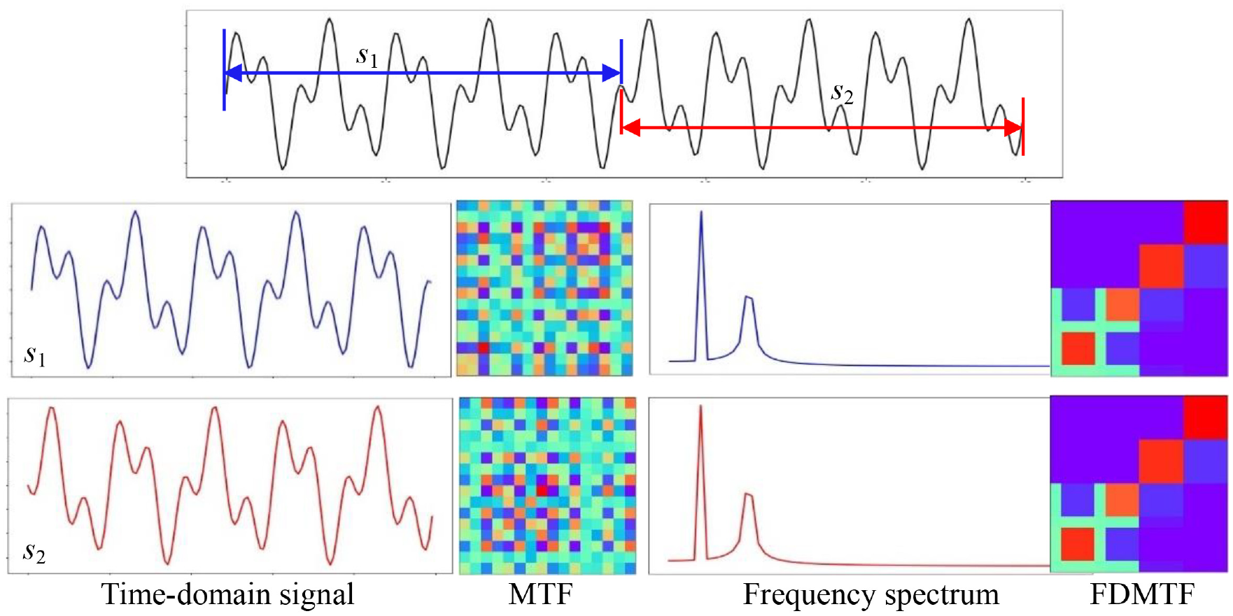
The comparison between MTF and FDMTF.

As shown in Figure 1, signals s₁ and s₂ differ in phase, resulting in differences in their time-domain MTF diagrams. Not only their spectrums but also their FDMTF images are identical. Figure 1 shows that FDMTF has more advantages in encoding signals to images than time-domain MTF. The obvious reason is that FDMTF can resist the influence of the phase change of the signal, while MTF cannot.

The proposed fault diagnosis method

A new QCC gearbox fault diagnosis method is proposed in this section. The process of the proposed method is drawn in Figure 2.

Figure 2.

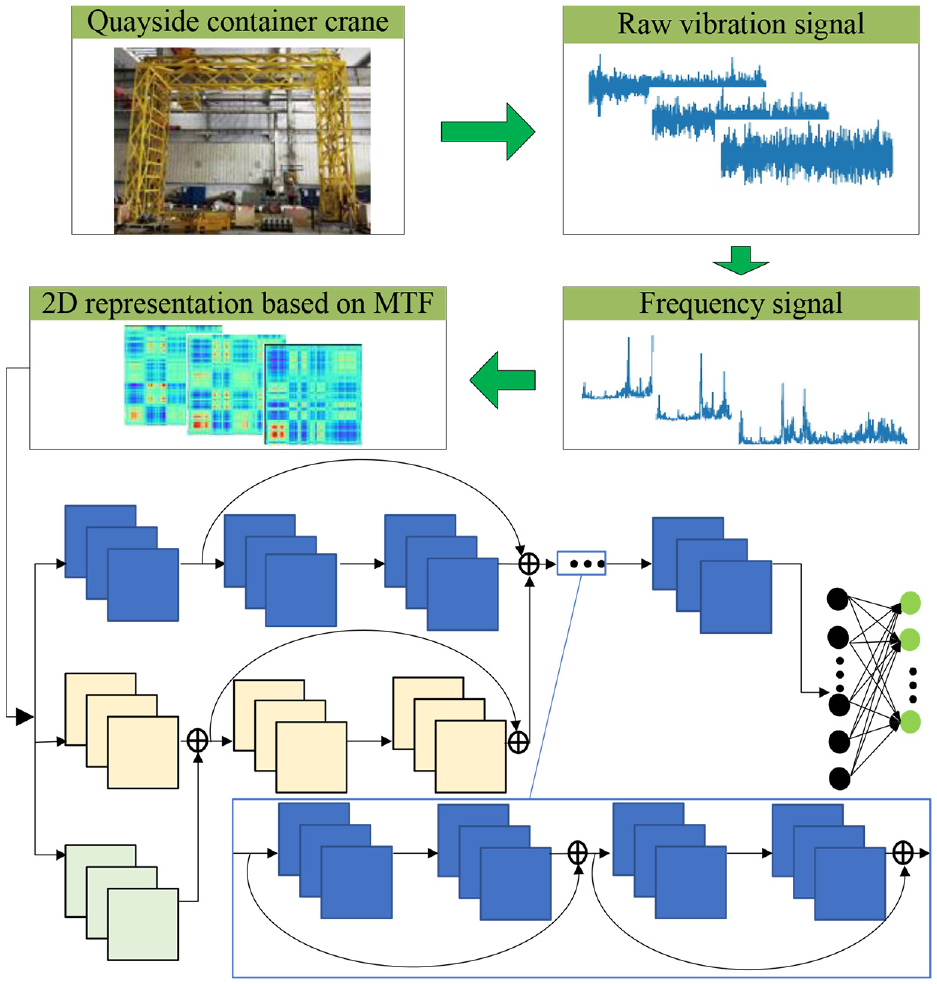
The process of FDMTF–MBRCNN.

Figure 2 covers the main establishment steps of the proposed FDMTF–MBRCNN method, including the acquisition of FDMTF and the construction of the CNN network structure, that is, MBRCNN. The proposed FDMTF–MBRCNN method is used to classify online vibration signals into a certain category to complete fault diagnosis by training historical vibration signals. This method first converts the vibration signal into the FD and then obtains the FDMTF based on the FD signal, which is used as the input of MBRCNN. MBRCNN consists of nine layers, which integrates the MB block of GoogLeNet and the residual block of ResNet. There are three branches designed, and the length of each branch is different. The first branch has eight network layers, the second branch has three network layers and the third branch has only one network layer. The size of the initial convolution kernel is related to different levels of original features. To obtain different levels of original features, the size of the first convolution kernel of the three branches is inconsistent. The extracted features from the third branch converge to the second branch. Similarly, the extracted features from the second branch converge in the first branch. In this way, the MBRCNN model can extract rich features at different levels. The residual module uses two network layers.

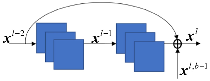
There are no residual modules in the third branch, one residual module in the second branch and three residual modules in the first branch. The basic MBRCNN module involving two branches and a residual module is shown in Figure 3.

Figure 3.

The basic module of MBRCNN.

It can be seen from Figure 3 that the output of layer l, x ^l comes from three aspects: one is the feature of layer l − 2, x ^l-2 obtained by using shortcut connection, one is the output of layer l − 1, x ^l − 1 of ordinary connection and another is x ^{l, b − 1} from the branch of b − 1. The output of layer l is expressed as follows:

x^{l} = σ [(ω * x^{l - 1} + b) + x^{l - 2} + x^{l, b - 1}]

(6)

where ω represents the weight of the interaction with the x ^l − 1, and b represents the offset of the layer l.

How to obtain FDMTF and the advantages of FDMTF over MTF have been introduced in section ‘The frequency-domain MTF’. To facilitate a clear understanding, this section focuses on the MBRCNN construction, and the specific steps of the proposed fault diagnosis method for the QCC gearbox.

The constructed CNN model

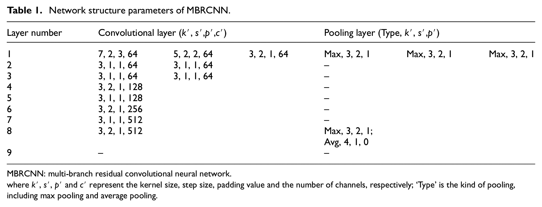
According to Figure 2, we introduce the MBRCNN model in detail. The specific details of the network, such as the size of the convolution kernel and the output channel, can be seen in Table 1.

Table 1.

Network structure parameters of MBRCNN.

Layer number	Convolutional layer (k′, s′,p′,c′)			Pooling layer (Type, k′, s′,p′)
1	7, 2, 3, 64	5, 2, 2, 64	3, 2, 1, 64	Max, 3, 2, 1	Max, 3, 2, 1	Max, 3, 2, 1
2	3, 1, 1, 64	3, 1, 1, 64		–
3	3, 1, 1, 64	3, 1, 1, 64		–
4	3, 2, 1, 128			–
5	3, 1, 1, 128			–
6	3, 2, 1, 256			–
7	3, 1, 1, 512			–
8	3, 2, 1, 512			Max, 3, 2, 1;Avg, 4, 1, 0
9	–			–

MBRCNN: multi-branch residual convolutional neural network.

where k′, s′, p′ and c′ represent the kernel size, step size, padding value and the number of channels, respectively; ‘Type’ is the kind of pooling, including max pooling and average pooling.

As can be seen from Table 1, MBRCNN designs multiple branches in the first three layers. The convolution kernels with different sizes are expected to extract the multi-scale features of the same input. For the general convolution layer, the convolution operation is expressed by the following formula.

x_{j}^{l} = σ (\sum_{c = 1}^{C} ω_{c, j}^{l} * x_{c}^{l - 1} + b_{j}^{l})

(7)

where $x_{j}^{l}$ is the output feature of the j-th channel at the l-th layer; σ(·) is the activation function; $ω_{c, j}^{l}$ is the convolution kernel interacting with the c-th channel at layer l − 1; $x_{c}^{l - 1}$ is the c-th channel feature at layer l − 1; $b_{j}^{l}$ is the corresponding bias. This article adopts ReLu(·) as the activation function. To further avoid the problems of overfitting under small samples and gradient disappearance/explosion caused by deep network structure, we use batch normalization (BN) operation for the convolution layer. It should be noted that the mean value is subtracted during the BN operation, and the bias term can be ignored or set to 0. Therefore, Equation (7) becomes:

x_{j}^{l} = ReLu (BN (\sum_{c = 1}^{C} ω_{c, j}^{l} * x_{c}^{l - 1}))

(8)

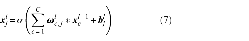
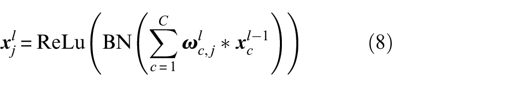
where ReLu(·) is the activation; BN represents the batch normalization operation.

The convolution operation of the basic MBRCNN module can be expressed by the general formula.

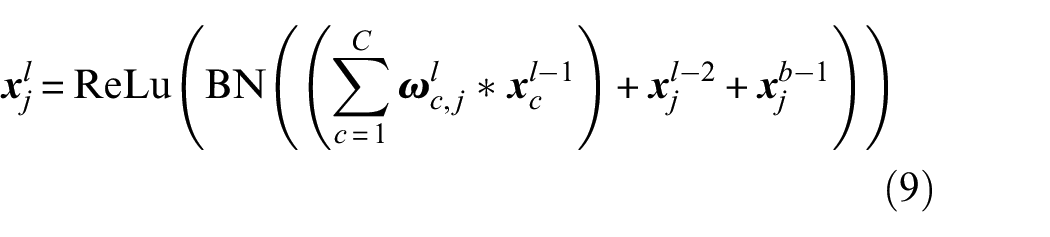
x_{j}^{l} = ReLu (BN ((\sum_{c = 1}^{C} ω_{c, j}^{l} * x_{c}^{l - 1}) + x_{j}^{l - 2} + x_{j}^{b - 1}))

(9)

where $x_{j}^{l - 2}$ is the output feature of layer l − 2; $x_{j}^{b - 1}$ is the output feature of the near branch. Herein, when different branches and residual blocks are connected under the condition of different feature sizes and channels, the 1 × 1 convolution layer is used to eliminate the difference in connection.³⁵

The pooling layer generally follows the convolution layer to reduce the dimension of the feature map. Because it does not involve parameter updating, it is not necessary to regard it as an independent network layer. The MBRCNN constructed in this article adopts two pooling operations, that is, max pooling and average pooling. The pooling process is briefly described as follows:

x_{j}^{l} = down (x_{j}^{l}, d)

(10)

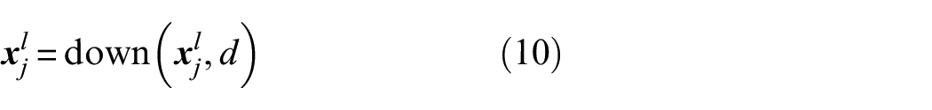
where $x_{j}^{l}$ represents the pooling operation, and d is the pooling size. Max pooling and average pooling output the maximum and average values among the area of d × d in the feature map, respectively.

The last layer of the MBRCNN is the full connection layer, which uses Softmax (·) as the activation function.

Softmax (u_{i}) = e^{u_{i}} / \sum_{o = 1}^{O} e^{u_{q}}

(11)

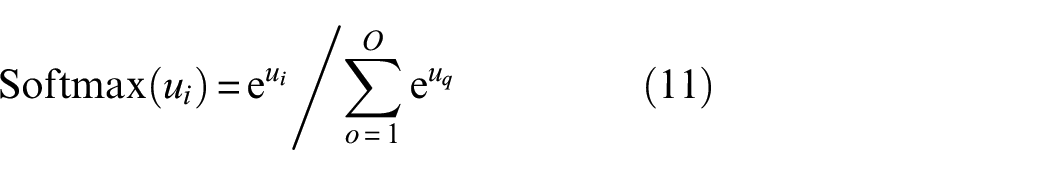
where u_i is the output value of the i-th node of the front unit of the classifier, o is the index of the number of nodes and O is the total number of categories, o∈[1, O].

The cross-entropy is selected as the loss function as the training goal.

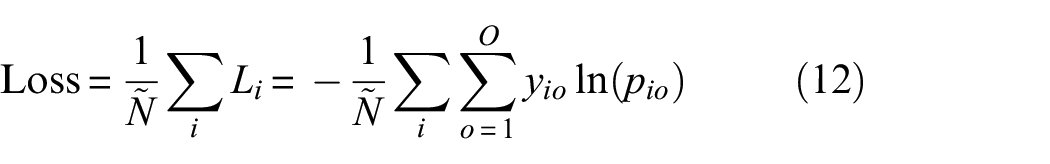
Loss = \frac{1}{\tilde{N}} \sum_{i} L_{i} = - \frac{1}{\tilde{N}} \sum_{i} \sum_{o = 1}^{O} y_{io} \ln (p_{io})

(12)

where $\tilde{N}$ is the total number of training samples; L_i is the loss of sample i; y_io is a symbolic function; when the category is m′, the symbolic function y_im_′ is 1, otherwise it is 0; p_io is the probability value of sample i belonging to category o obtained by using softmax function.

The steps of the FDMTF–MBRCNN method

The flowchart of the FDMTF–MBRCNN method for QCC gearbox fault diagnosis is shown in Figure 4. The step of data preparation in the diagnosis process using online data is the same as that in the training step.

Figure 4.

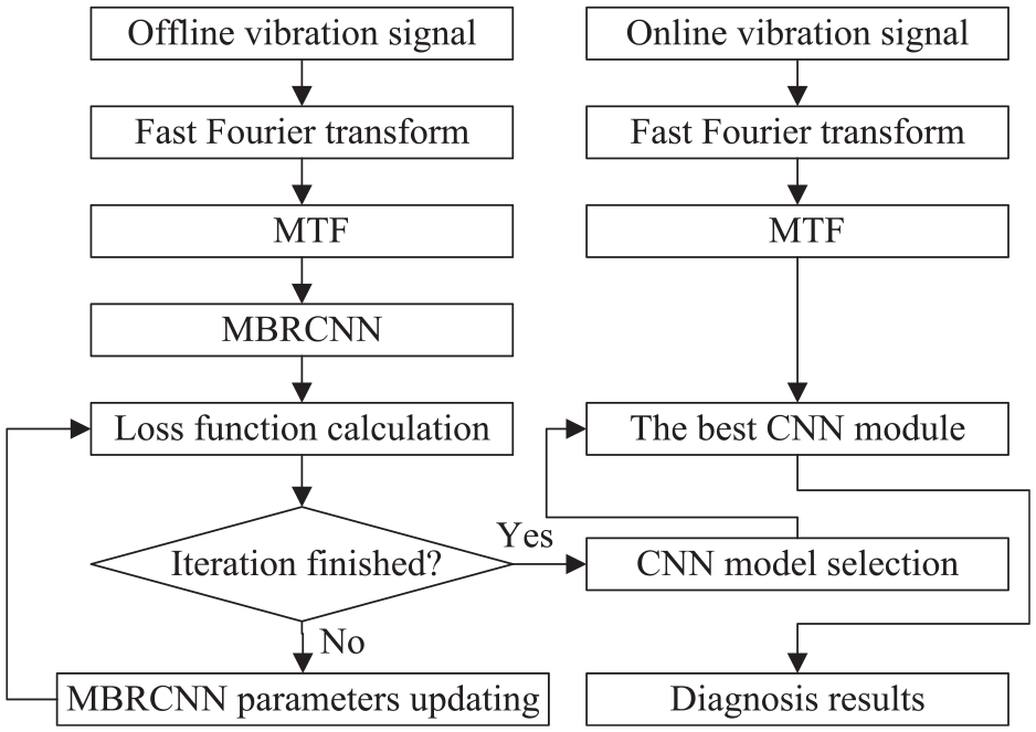
The flowchart of the FDMTF–MBRCNN for gearbox diagnosis.

According to Figure 4, the steps of the proposed FDMTF–MBRCNN method for the QCC gearbox fault diagnosis are as follows:

Step 1: Offline signal collection. Collect the vibration signals of the QCC gearbox with different statuses.

Step 2: Image representation. The collected vibration signals are first subjected to fast Fourier transform, then the FD signal is encoded by MTF to obtain FDMTF according to section ‘The frequency-domain MTF’.

Step 3: MBRCNN model construction. Integrate muti-branch blocks and residual blocks to construct MBRCNN according to section ‘The constructed CNN model’.

Step 4: The network loss function calculation. Divide the training set into two parts, one of which is used to calculate the loss function according to Equation (12).

Step 5: Iteration judgement. If the number of iterations is reached, go to Step 7; If it is less than the number of iterations, proceed to Step 6.

Step 6: Parameters updating. Use the Adam method³⁸ to optimize network parameters. After updating all network parameters, get the network model belonging to this iteration and return to Step 4.

Step 7: CNN model selection. Input the remaining part of the training set, that is, the validation set into the network model of each iteration to identify the iterative model with the highest accuracy as the final trained model.

Step 8: Online diagnosis. obtain the FDMTF of the online vibration signal, and then input it to the trained model obtained in Step 7 to get the diagnosis results.

Case study

There are two case studies used to prove the effectiveness of the FDMTF–MBRCNN method. The gearbox dataset of Case 1 is provided by the University of Connecticut (UoC),^39,40 which has been extensively used to explore the performance of fault diagnosis methods.^41–48 In addition, Zhao et al.⁴¹ tested seven publicly available datasets through four benchmark types of deep learning models and showed that the UoC gearbox dataset is the most difficult to diagnose among the seven datasets. The gearbox data of Case 1 is used to study the universality and progressiveness of the proposed method. The gearbox data of Case 2 is collected from a scaled-down test rig of QCC, which is the main case study of this article because it is closer to the real QCC gearbox dataset.

Case 1: UoC gearbox dataset

The UoC gearbox dataset is collected from a benchmark two-stage parallel shaft gearbox test rig. The faulty gear is located on the input shaft of the first stage. The vibration signals of the gearbox in nine different statuses are collected by the accelerometer sensor. In addition, the dataset used in Case 1 is provided by Cao et al.^39,40 which does not describe its operating conditions in detail, so Case 1 is not considered proof of diagnosis under variable loads. The length of the acquired signal is 3600, and the corresponding sampling frequency of 20 kHz. The vibration signals of nine statuses are all used for analysis, including normal, tooth missing, tooth root crack, tooth spalling and tooth chipping (five different fault levels). The sample label of each gear status and the corresponding sample quantity is shown in Table 2.

Table 2.

The labels of different gear statuses.

Label	The health status	The number of samples
1	Normal	104
2	Tooth missing	104
3	Tooth root crack	104
4	Tooth spalling	104
5	Tooth chipping with level 5	104
6	Tooth chipping with level 4	104
7	Tooth chipping with level 3	104
8	Tooth chipping with level 2	104
9	Tooth chipping with level 1	104

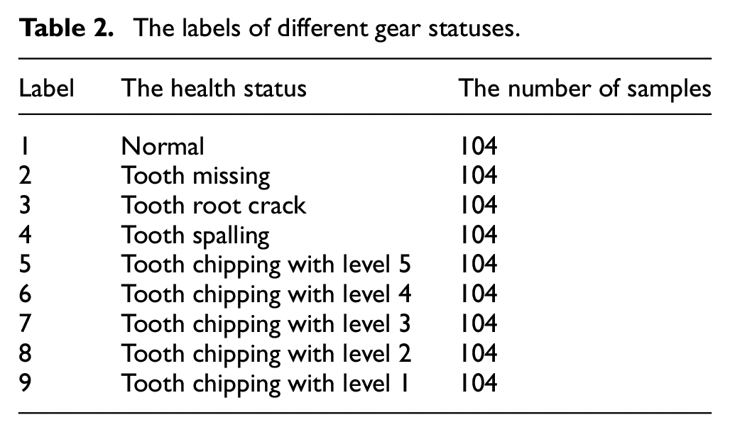
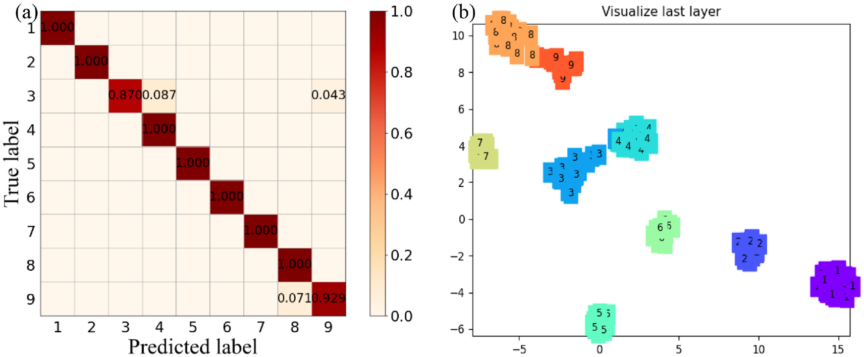
In Table 2, chipping with level 1 represents the most serious chipping fault, and on the contrary, chipping with level 5 represents the least serious fault. About 104 samples were collected in each gear status, so there are 936 samples in total. Herein, according to the ratio of 7:3, the training set and testing set are randomly divided. Among the training set, 0.55 × 936 is used as the training part, and 0.15 × 936 is used as the validation part. The image size of the input MBRCNN model is 224 × 224. The training hyper-parameters are set as follows: the mini-batch size, the learning rate and the number of epochs are set to 64, 0.001 and 20, respectively. To illustrate the learning ability of MBRCNN, t-distributed stochastic neighbour embedding (t-SNE)⁴⁹ is used to visualize the feature of the last layer before the full connection layer. The recognition accuracy of the UoC gearbox dataset is 100%, which fully demonstrates the availability of the FDMTF–MBRCNN method. The specific diagnosis results are drawn in Figure 5.

Figure 5.

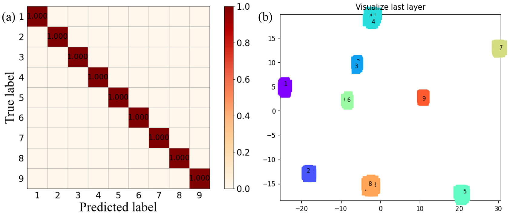
The diagnosis results: (a) the recognition accuracy and (b) dimensionality reduction representation of features by t-SNE.

Figure 5(a) is the confusion matrix of the diagnosis results, indicating that the correct recognition rate of each category is 100%. Figure 5(b) shows that different kinds of samples are well-distinguished without overlapping, which proves the feature extraction ability of MBRCNN. To avoid accidental interference, the dataset was trained and tested five times. The recognition accuracy is still 100% each time, which proves the stability of the proposed method.

Comparison analysis of Case 1

Based on the UoC gearbox dataset, the proposed FDMTF–MBRCNN is compared with other state-of-the-art methods published in recent 3 years. Many pieces of literature use this dataset for fault diagnosis under limited training samples. To facilitate comparison, the diagnosis results of the proposed method are also carried out under different training sample quantities. It should be noted that some literatures have expanded the total amount of data to meet the requirements for training. The detailed comparison results are shown in Table 3.

Table 3.

The details of the comparison results.

Source	Year of publication	Method description	Proportion of training set	Number of samples	Averageaccuracy
Jin et al.⁴²	2022	Time series transformer-based method	70%	936	0.9951
Lu et al.⁴³	2021	Optimized stacked diagnosis structure	70%	936	0.9924
Qian and Liu⁴⁴	2022	CNN-RL/GRU-RL	10%	936 × 2	0.928/0.989
Qian and Liu⁴⁵	2022	CGAN–MLP	10%	936 × 2	0.996
Fu et al.⁴⁶	2022	Task-incremental broad learning system	86.5%	936 × 10	0.9302
Hu et al.⁴⁷	2020	Redefined dimensionless indicatorsand mRMR	67.3%	936	0.9712
Shao et al.⁴⁸	2022	Modified SAE	72% (17% Validation)	936 × 3	0.9886
This article	_	FDMTF–MBRCNN	70% (15% Validation)	936	1
			50% (15% Validation)	936	1
			40% (15% Validation)	936	1
			30% (15% Validation)	936	1
			20% (10% Validation)	936	1
			10% (No Validation)	936	1

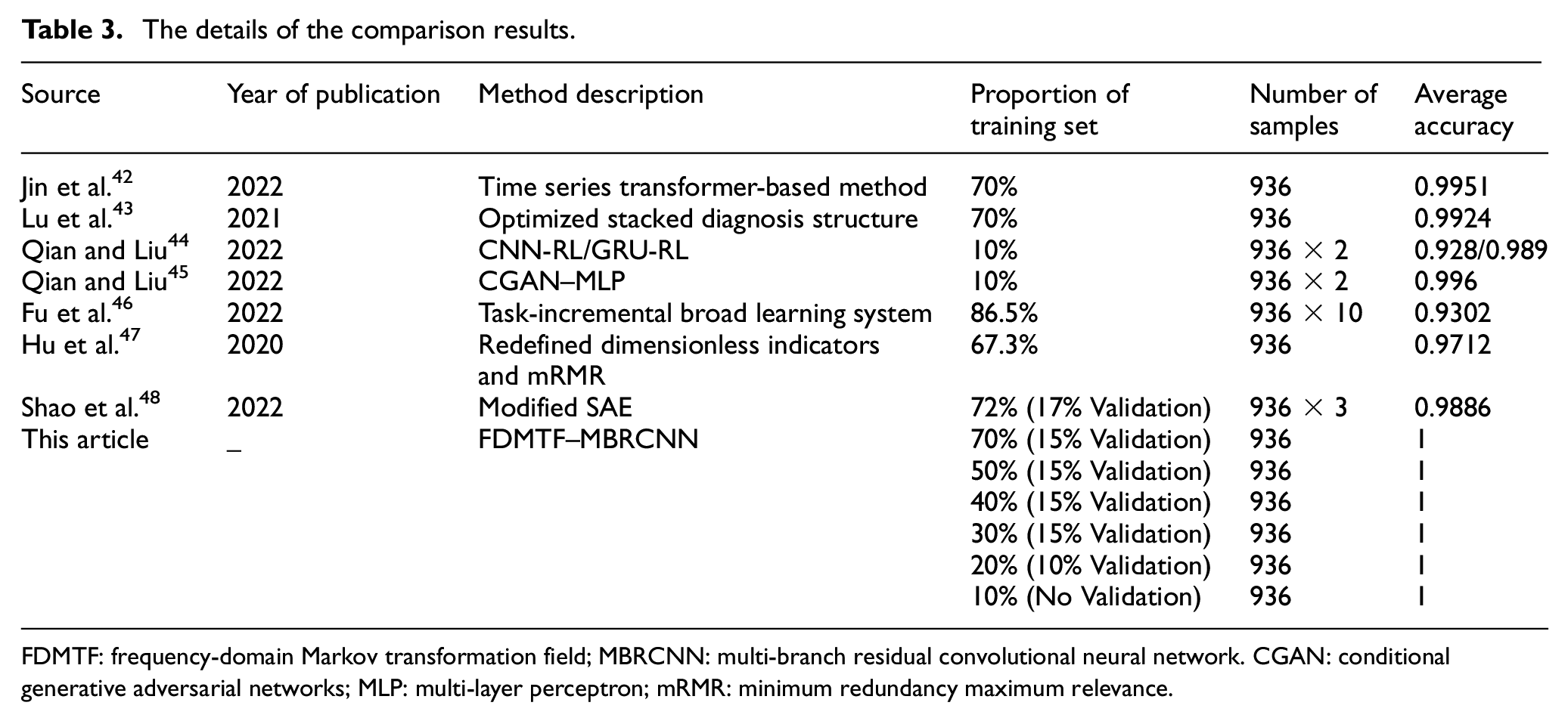
FDMTF: frequency-domain Markov transformation field; MBRCNN: multi-branch residual convolutional neural network. CGAN: conditional generative adversarial networks; MLP: multi-layer perceptron; mRMR: minimum redundancy maximum relevance.

In Table 3, the proportion of the training set includes the samples of all known labels, including training samples and validation samples. Jin et al.⁴² proposed two methods, that is, CNN-RL and gated recurrent unit neural network -reinforcement learning, which obtained recognition accuracy of 0.928 and 0.989, respectively. On the one hand, Table 3 shows the recognition accuracy of the FDMTF–MBRCNN under different proportions of training datasets. The recognition accuracy of the proposed method is 100% under different training proportions of 10%, 20%, 30%, 40%, 50% and 70%, which proves its robustness. In addition, it shows that the FDMTF–MBRCNN method can achieve good results with the small sample problem. According to Zhang et al.⁵⁰ if the proportion of the training set is less than 50%, it can be regarded as a small sample problem. On the other hand, these diagnosis results fluctuate in the range of 0.929–0.996 obtained by the methods proposed in different literatures based on UoC gearbox dataset, without exception, less than the recognition accuracy of the proposed FDMTF–MBRCNN method. The comparison results in Table 3 prove the superiority of the FDMTF–MBRCNN method.

Case 2: QCC gearbox dataset

To collect the QCC gearbox vibration signal, we built a scaled-down test rig of an actual type of QCC with a ratio of 1:4, as shown in Figure 6.

Figure 6.

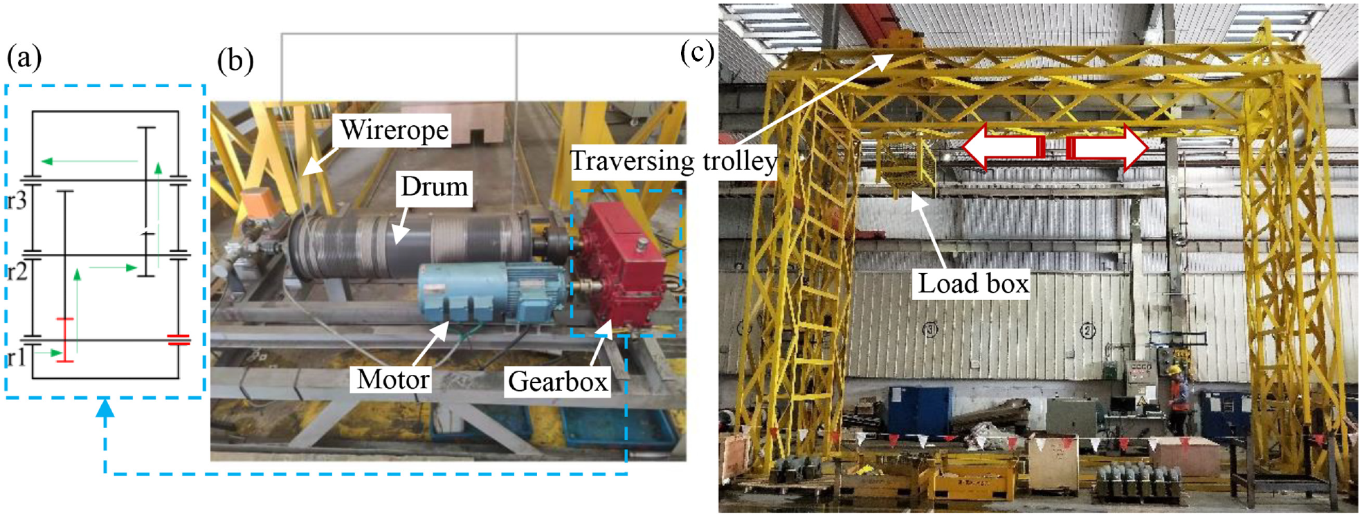
The scaled-down test rig of a QCC: (a) the location of faulty parts, (b) the trolley movement gearbox and (c) the appearance of the test rig.

The movement of the load box controlled by the test rig is divided into vertical and horizontal movement to simulate the operation of loading and unloading container ships. Therefore, the power output of the whole test rig is divided into two parts, and the two motors are connected to the corresponding gearbox, respectively. The trolley gearbox controls the horizontal movement of the load box. The hoisting gearbox controls the vertical movement. In the experiment, the running statuses of the trolley gearbox are used to research. Figure 6(a) shows the location of the faulty parts of the trolley gearbox. The red position is where the parts are located, and the green line reflects the power transmission inside the gearbox. Figure 6(b) shows the appearance of the horizontal trolley gearbox, which is the object of this experiment. It can be seen that the motor provides power, and the power is transmitted to the horizontal movement of the trolley driven by the steel wire rope through the drum and gearbox. Figure 6(c) shows the appearance of the test rig. The load box is added with iron blocks to simulate the actual containers. During the experiment, the input speed of the trolley gearbox is 1750 rpm, and the load is 1000 kg. The number of sampling points is 2048 with the sampling frequency = 10,000 Hz.

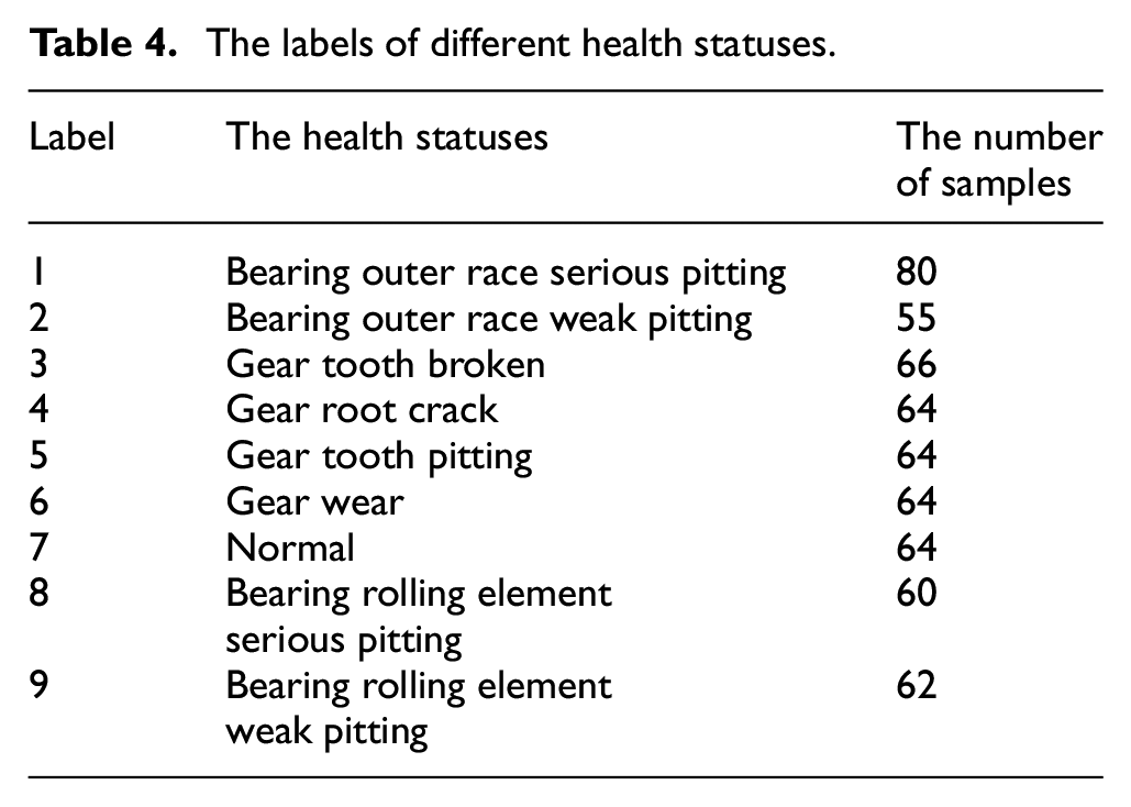
The vibration signals of the gearbox under nine different health statuses are collected. The specific category label of each health status, and the corresponding number of samples are shown in Table 4. A total of 579 samples were obtained in the experiment.

Table 4.

The labels of different health statuses.

Label	The health statuses	The numberof samples
1	Bearing outer race serious pitting	80
2	Bearing outer race weak pitting	55
3	Gear tooth broken	66
4	Gear root crack	64
5	Gear tooth pitting	64
6	Gear wear	64
7	Normal	64
8	Bearing rolling element serious pitting	60
9	Bearing rolling elementweak pitting	62

The faulty parts used in Case 2 are shown in Figure 7. For the convenience of observation, we mark the damage location with a green circle. In addition, the broken tooth and worn tooth shall be coated with pink paint.

Figure 7.

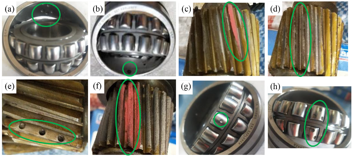
The faulty parts of Case 2: (a)–(f): Label 1–6 and (g), (h): label 8, 9.

Figure 7 shows the eight fault types analysed in Case 2. We randomly extract six signals under the normal status and show their time-domain waveform, spectrum, time-domain MTF and FDMTF in Figure 8.

Figure 8.

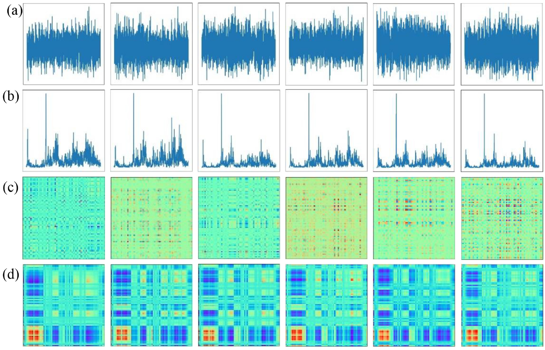
Four different 2D expressions of the 1D vibration signal under normal status: (a) time-domain image, (b) frequency-domain image, (c) time-domain MTF and (d) FDMTF.

The images shown in Figure 8(a) as well as Figure 8(c) which are obtained by the time-domain signal perform poorly because there are large differences between images even for the same health status. It may reveal that the vibration signal of the scaled-down test rig is subject to unknown interferences. Figure 8(b) and (d) based on the FD signal shows that the six images are almost consistent in the same state, respectively. Figure 8 shows that the FDMTF that can resist the impact of unknown interferences is more robust than the time-domain MTF.

The images of FDMTF in nine different health statuses are shown in Figure 9. The FDMTF presents different expressions under different health statuses of the gearbox, which is conducive to the training of MBRCNN. Combining Figures 8 and 9, one can find that the FDMTF is suitable for encoding the gearbox vibration signal into the 2D image. The reason lies in that FDMTF can make the images of the same health state similar, and the images of different health state differential.

Figure 9.

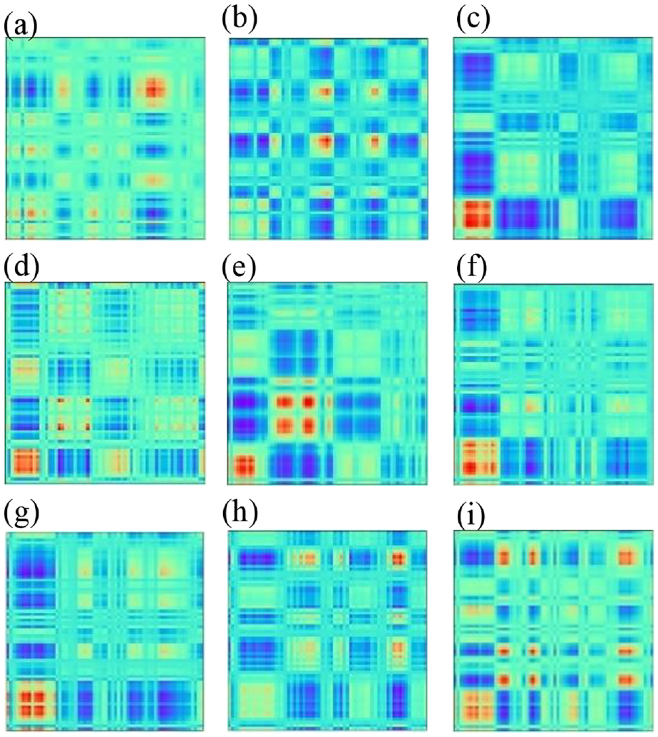
The FDMTF of the vibration signals under nine statuses: (a)–(i) corresponding to the label 1–9.

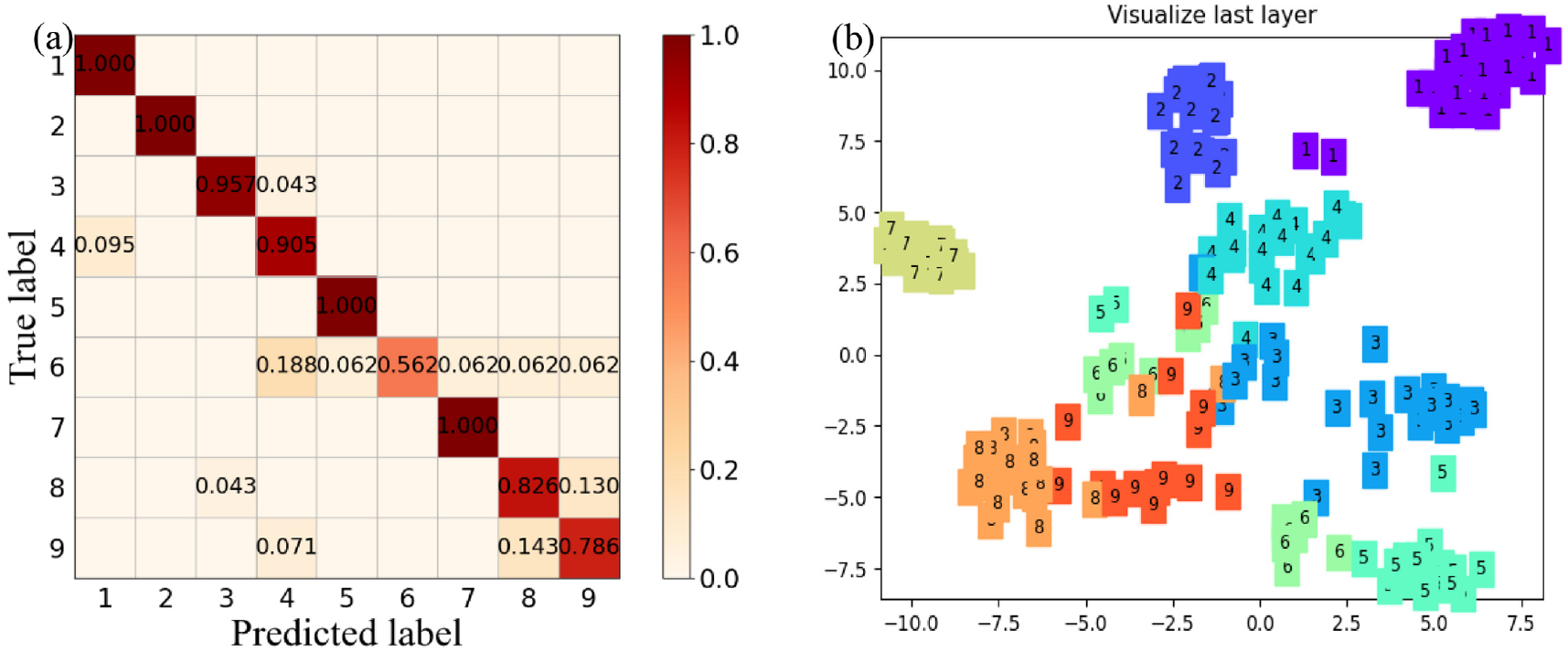
Carry out training and testing according to the steps of the FDMTF–MBRCNN method in section ‘The steps of the FDMTF–MBRCNN method’. The training sample proportion, network hyper-parameters and input image size are the same as those of Case 1. According to the previous deployment, a total of 174 samples participated in the test. The overall recognition accuracy is 98.85%, and the specific diagnosis results are shown in Figure 10. Figure 10(a) shows that only two samples of gear tooth broken are mistaken for gear root crack. The identification accuracy of the remaining categories is 100%. Figure 10(b) shows that the features extracted by MBRCNN are very effective and can separate different kinds of samples. To eliminate the influence of accidental factors, we have trained and tested five times. The recognition accuracies of all five tests are also 98.85%, which proves the stability of the proposed method.

Figure 10.

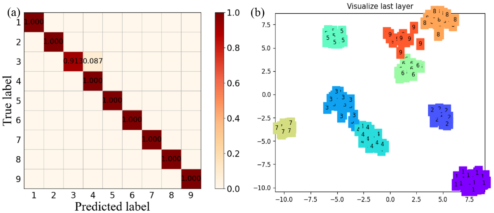
The diagnosis results: (a) the recognition accuracy and (b) dimensionality reduction representation of features by t-SNE.

Comparison analysis of Case 2

The comparison with FDMTF

To prove the merits of the proposed method in 2D characterization, other methods that can characterize 1D vibration signals into 2D images are used to compare with FDMTF. These methods include time-domain MTF, spectrum, time-domain waveform, FD GADF, time-domain GADF, FDGASF, time-domain GASF, FDRP, time-domain RP, STFT and CWT. As mentioned in the introduction part, most of these 2D encoding methods have been used in fault diagnosis. Input these different 2D characterization images into MBRCNN, and the diagnosis results are shown in Table 5. For convenience, the standard deviation is placed behind the average recognition accuracy to describe the dispersion of the average value.

Table 5.

The diagnosis results of different inputs based on MBRCNN.

Input	Diagnosis accuracies of different training times					Average accuracy
Input	1	2	3	4	5	Average accuracy
FDMTF	0.9885	0.9885	0.9885	0.9885	0.9885	0.9885 ± 0
Time-domain MTF	0.1149	0.1609	0.1609	0.2069	0.2069	0.1701 ± 0.0385
Frequency spectrum	0.9713	0.9885	0.9828	0.977	0.9828	0.9805 ± 0.0065
Time-domain waveform	0.3276	0.3563	0.3333	0.3506	0.3448	0.3425 ± 0.0119
Frequency-domain GADF	0.9828	0.9828	0.9828	0.9828	0.9828	0.9828 ± 0
Time-domain GADF	0.3391	0.3161	0.2759	0.3391	0.3276	0.3196 ± 0.0262
Frequency-domain GASF	0.9828	0.9828	0.977	0.9828	0.9828	0.9816 ± 0.0026
Time-domain GASF	0.1667	0.2011	0.1839	0.1667	0.1552	0.1747 ± 0.018
Frequency-domain RP	0.9425	0.9368	0.9483	0.931	0.9368	0.9391 ± 0.0066
Time-domain RP	0.3506	0.2759	0.2184	0.3161	0.3218	0.2966 ± 0.0512
Time-domain–frequency-domain STFT	0.977	0.9655	0.9713	0.9826	0.9885	0.977 ± 0.0091
Time–frequency-domain CWT	0.9023	0.9138	0.9023	0.9195	0.9138	0.9103 ± 0.0077

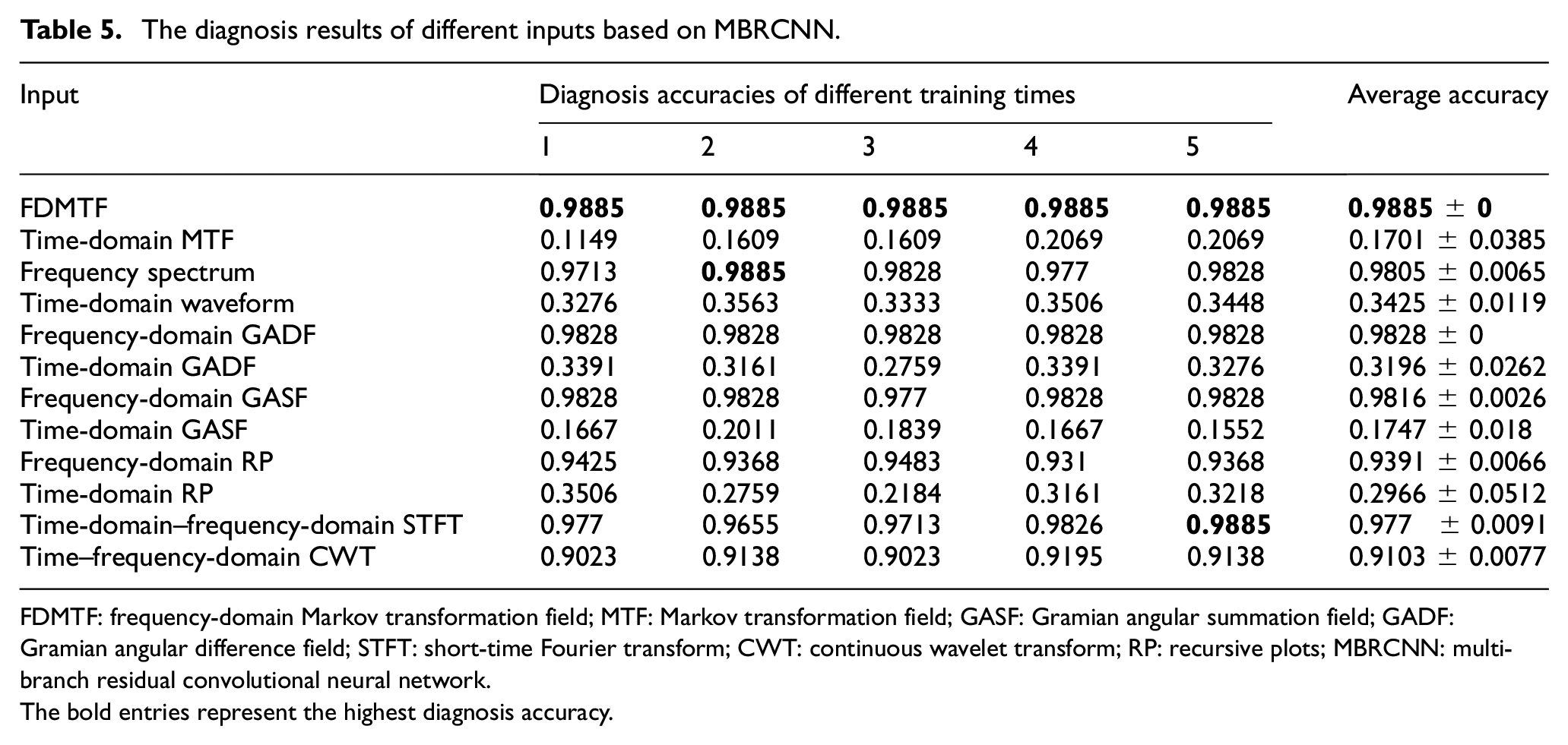
FDMTF: frequency-domain Markov transformation field; MTF: Markov transformation field; GASF: Gramian angular summation field; GADF: Gramian angular difference field; STFT: short-time Fourier transform; CWT: continuous wavelet transform; RP: recursive plots; MBRCNN: multi-branch residual convolutional neural network.The bold entries represent the highest diagnosis accuracy.

Table 5 shows that the diagnosis accuracy of 98.85% of the proposed FDMTF is higher and more stable than the other 11 methods, which proves the superiority of using FDMTF as the input of MBRCNN. The recognition accuracy of the spectrum, FDGADF, FDGASF, FDRP, STFT and CWT can reach more than 90%. However, the recognition accuracy of the methods that directly encode time-domain information to the 2D image including time-domain waveform, time-domain MTF, time-domain GADF, time-domain GASF and time-domain RP, which obtain poor diagnosis results, is less than 35%. The reason may lie in that the time-domain vibration signal is prone to be disturbed by the phase, background noise, etc., resulting in large differences in the signals even under the same state. To further show the difference between the 2D representation methods based on FD signals and time-domain signals, we draw the average recognition accuracy in Table 5 into Figure 11.

Figure 11.

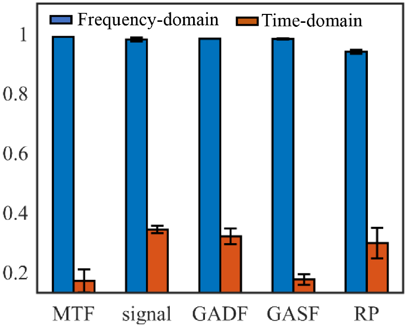
The comparison of recognition accuracy based on time domain and frequency domain.

In Figure 11, the signal means the raw vibration signal. Figure 11 intuitively shows the difference in the recognition results obtained by encoding 2D images based on FD signals and time-domain signals. The five different encoding methods tend to convert the FD signal rather than the time-domain signal into the 2D image as the input of MBRCNN to obtain higher recognition accuracy.

The comparison with MBRCNN

To prove the advantages of MBRCNN in feature extraction and classification, the famous networks AlexNet and ResNet-18 are used as diagnosis models for comparison. Using FDMTF as input, the recognition results obtained by AlexNet and ResNet-18 are drawn in Figures 12 and 13, respectively.

Figure 12.

The fault diagnosis results of AlexNet: (a) the recognition accuracy and (b) dimensionality reduction representation of features by t-SNE.

Figure 13.

The fault diagnosis results of ResNet-18: (a) the recognition accuracy and (b) dimensionality reduction representation of features by t-SNE.

The recognition accuracy of AlexNet is 90.23%, and that of ResNet-18 is 97.7%. The recognition accuracy of the above two network models is lower than that of the proposed method, which proves the advantages of MBRCNN. At the same time, AlexNet as well as ResNet-18 can obtain recognition accuracy of more than 90%, which shows that FDMTF is suitable for the characterization of the 1D vibration signal. Figures 12(b) and 13(b) show that the feature extraction ability of AlexNet and ResNet-18 is also weaker than that of MBRCNN in this case analysis.

To further prove the advantages of the proposed MBRCNN model, ImageNet⁵¹ which is widely used to assist in CNN model training is used to pre-training as well as fine-tuning ResNet-18. The strategy of pre-training refers to using the model parameters trained by other datasets as the initial initialization parameters to replace the random parameters. The method of fine-tuning refers to the use of network parameters trained by other datasets as the parameters of the feature extraction layer. It is no longer necessary to update and optimize the feature extraction layer, while only adjusting the parameters of the full connection layer slightly for the strategy of fine-tuning.

Therefore, ResNet-18 has three training strategies, including training directly whose results are shown in Figure 13, pre-training and fine-tuning. To eliminate accidental factors, each method was trained and tested five times. The average recognition accuracy obtained by the abovementioned methods is shown in Table 6.

Table 6.

The average recognition accuracy of different network models.

Methods	The proposed method	AlexNet	ResNet-18
			Training directly	Pre-training	Fine-tuning
Accuracy	0.9885 ± 0	0.9023 ± 0	0.977 ± 0.0041	0.9655 ± 0	0.6379 ± 0

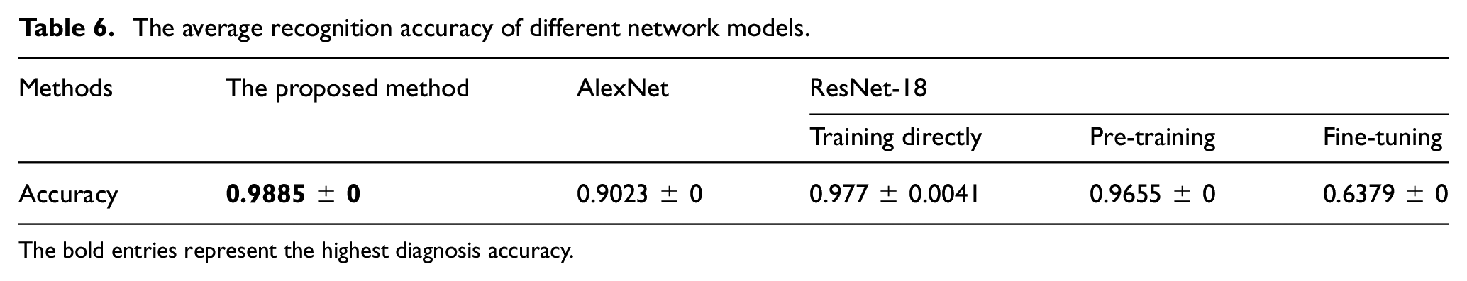
The bold entries represent the highest diagnosis accuracy.

Table 6 shows that the recognition accuracy of the proposed method is the highest at 98.85% among the five methods. The recognition accuracy of ResNet-18 training assisted by ImageNet is not higher than that of training directly, but lower. The recognition accuracy of fine-tuning is only 0.6379, which shows that the training strategy of fine-tuning is not suitable for fault diagnosis based on FDMTF.

Robustness analysis based on Case 2

Robustness against proportions of training sample

In subsection ‘Comparison analysis of Case 1’, the proposed method can achieve 100% recognition accuracy of the UoC dataset under the condition of a small training sample. The dataset of the QCC test rig may be more sensitive to the number of samples because the collected data contains noises and impact interferences.⁵² This subsection mainly proves the generalization performance of the FDMTF–MBRCNN method under different proportions of training samples. The corresponding diagnosis results are shown in Table 7.

Table 7.

The diagnosis results under different proportions of training samples.

Proportions of training set	Diagnosis accuracies of different training times					Average accuracy
Proportions of training set	1	2	3	4	5	Average accuracy
70% (15% Validation)	0.9885	0.9885	0.9885	0.9885	0.9885	0.9885 ± 0
50% (15% Validation)	0.9724	0.9759	0.9759	0.9724	0.9724	0.9738 ± 0.0019
40% (15% Validation)	0.9569	0.954	0.9569	0.954	0.954	0.9552 ± 0.0016
30% (No Validation)	0.9581	0.9581	0.961	0.9581	0.961	0.9593 ± 0.0016
25% (No Validation)	0.9563	0.9563	0.9586	0.9586	0.9563	0.9572 ± 0.0013

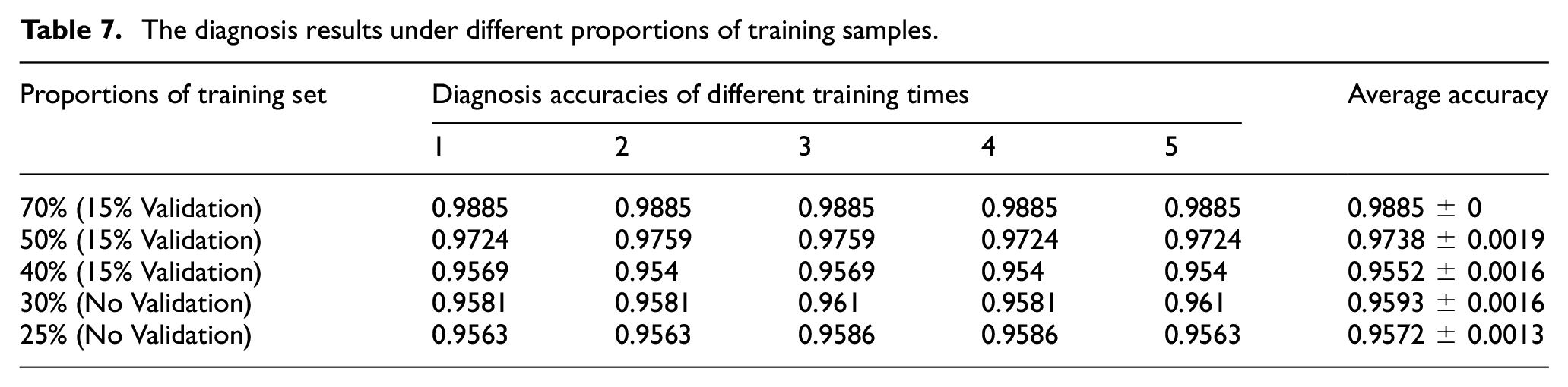
Due to the small amount of dataset obtained from the QCC test rig, when the proportion of training set is 30% and 25%, there is no verification set. When the proportion of training set is 25%–70%, the diagnosis accuracy is higher than 95%. The standard deviation of the proposed method can maintain a very small value in proportions of training set, which proves the stability of the proposed method. It proves the generalization and robustness against the proportion of training samples of the FDMTF–MNRCNN method. When the proportion of training samples is 25%, only 16 samples of each category participate in training on average, and a total of 435 samples are used for testing. In this case, the recognition accuracy of 0.9572 is still obtained, which again shows that the proposed method is expected to solve the small sample problem.

Robustness against hyper-parameters

The proposed method integrates the MB block and residual block. In addition to strong feature extraction ability, it can improve the insensitivity to hyper-parameters. MBRCNN has multiple branches with different depths, which may adapt to the different hyper-parameter settings. To prove the above surmise, we discuss the influence of three hyper-parameters, namely, the mini-batch size, the learning rate and the number of epochs, on the recognition accuracy. Herein, we adopt the control variable method, that is, when changing the preset value of one parameter, the values of the other two parameters remain unchanged. Similarly, to avoid the influence of accidental factors, each group of hyper-parameters is trained and tested five times. The average diagnosis recognition accuracy of five times when the three hyper-parameters are changed in turn is shown in Figure 14.

Figure 14.

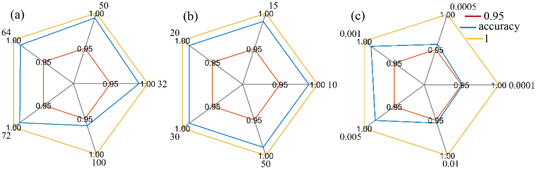
The recognition accuracies of changing hyper-parameters: (a) mini-batch size, (b) the number of epochs and (c) the learning rate.

The recognition accuracies under 15 different groups of hyper-parameter combinations are more than 95%, which proves that the proposed method is not sensitive to the setting of hyper-parameters. This shows that the MBRCNN model can adapt to different parameter combinations and reduce the complex action of parameter adjustment deep learning. It also can be seen that among the three parameters, the learning rate has a greater impact, and it is appropriate to choose a value near 0.001.

Robustness against variable loads

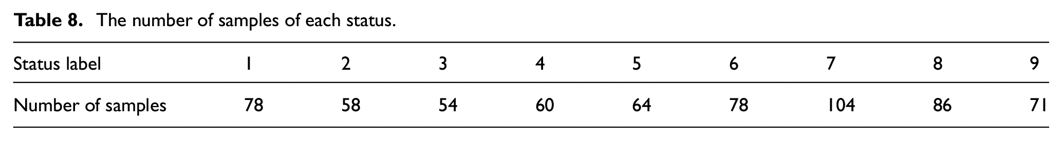
QCCs need to deliver containers of variable quality. The online vibration signal and training vibration signal are likely collected under different load conditions. To explore the robustness of the FDMTF–MBRCNN method against variable loads, the vibration signal of the test rig under 500 kg load conditions and 1750 rpm is collected for a new time. A total of 653 samples are collected. The detailed number of samples of each gearbox status is shown in Table 8.

Table 8.

The number of samples of each status.

Status label	1	2	3	4	5	6	7	8	9
Number of samples	78	58	54	60	64	78	104	86	71

In order to explain the influence of different operating conditions, taking normal vibration signal as an example, the time-domain waveforms and frequency spectrum under different load conditions are displayed in Figure 15.

Figure 15.

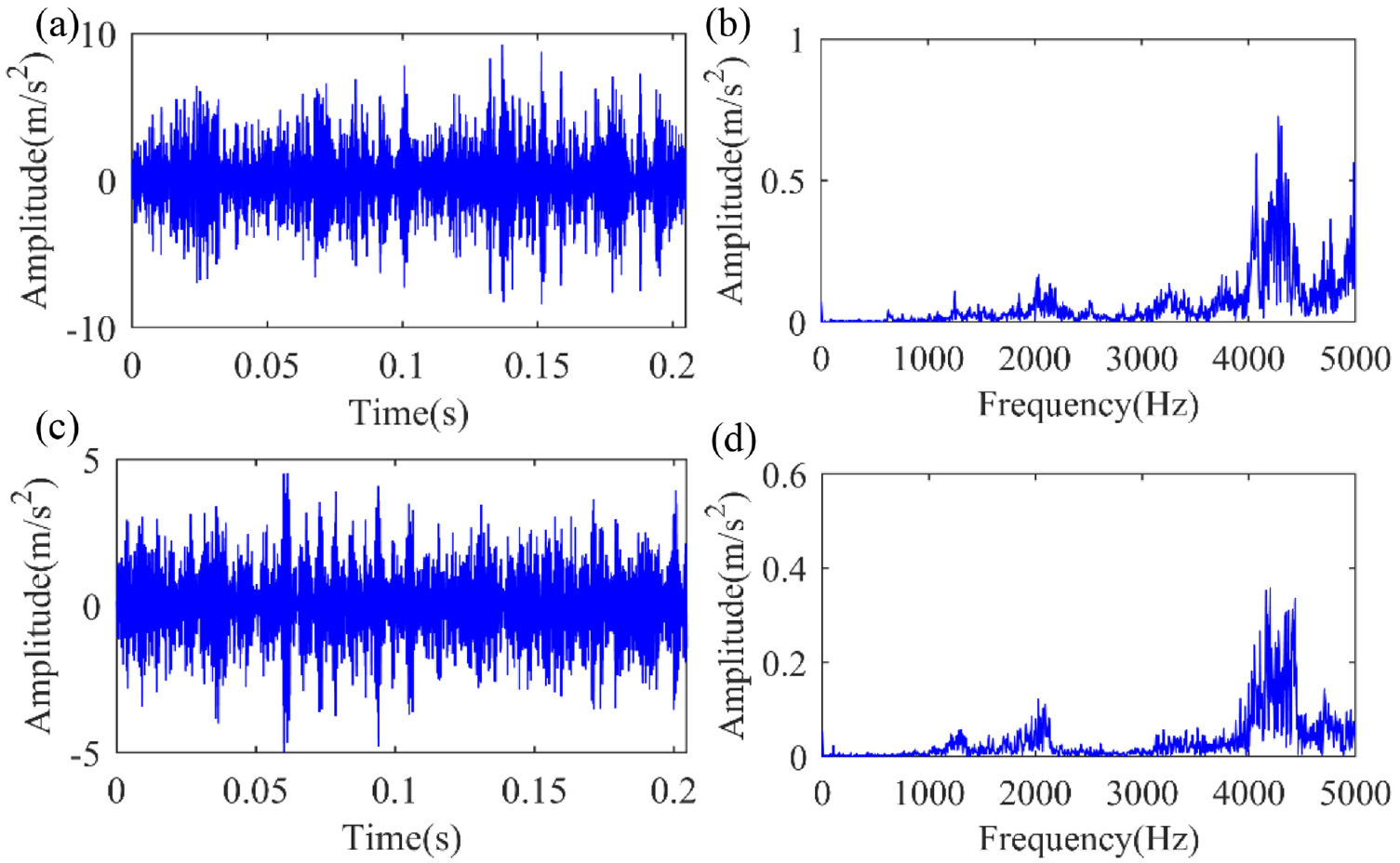
Time-domain waveform and spectrum under variable loads: (a) and (b) 1000 kg; (c) and (d) 500 kg.

Figure 15 shows that the amplitude under a load of 1000 kg is larger than that under a load of 500 kg, both in the time domain and the FD. It shows that the fluctuating operating load conditions will change the features of the vibration signal. All samples collected under 1000 kg load conditions are used to train the diagnosis models to diagnose the data collected at 500 kg load. During training, 70% of training set are used for training and the remaining 30% for validation to select the best model.

Based on the proposed FDMTF–MBRCNN method, the recognition accuracy of samples collected under a 500 kg load is 94.55%. On the one hand, this diagnosis result shows that the variable load does influence the recognition accuracy of the proposed method. On the other hand, it shows that the proposed method is robust against variable loads because the method still achieves 94.55% accuracy. Without the help of domain adaption technology, such a high recognition accuracy may be attributed to the good characterization of FDMTF. To highlight the advantages of FDMTF, other 11 characterization methods are also used to explore the possibility of fault diagnosis under variable loads. The specific diagnosis results are shown in Table 9.

Table 9.

The diagnosis results under variable load conditions.

Input	Diagnosis accuracies of different training times					Average accuracy
Input	1	2	3	4	5	Average accuracy
FDMTF	0.9449	0.9449	0.9479	0.9449	0.9449	0.9455 ± 0.0013
Time-domain MTF	0.1761	0.1501	0.1899	0.1608	0.1776	0.1709 ± 0.0156
Frequency- spectrum	0.8943	0.8989	0.9035	0.9005	0.902	0.8998 ± 0.0035
Time-domain waveform	0.2787	0.3262	0.3185	0.3247	0.3231	0.3142 ± 0.0201
Frequency-domain GADF	0.9081	0.9081	0.9096	0.9096	0.9066	0.9078 ± 0.0013
Time-domain GADF	0.2435	0.2588	0.2649	0.2328	0.2481	0.2496 ± 0.0127
Frequency-domain GASF	0.8867	0.8867	0.8897	0.8867	0.8882	0.8876 ± 0.0013
Time-domain GASF	0.1776	0.1761	0.173	0.1792	0.1409	0.1694 ± 0.0161
Frequency-domain RP	0.8821	0.879	0.8775	0.876	0.8821	0.8793 ± 0.0027
Time-domain RP	0.2711	0.2573	0.2221	0.2695	0.2619	0.2564 ± 0.02
Time-domain–frequency-domain STFT	0.8851	0.8867	0.8851	0.8851	0.8851	0.8855 ± 0
Time-domain–Frequency-domain CWT	0.7994	0.8193	0.8132	0.8162	0.8116	0.8119 ± 0.0076

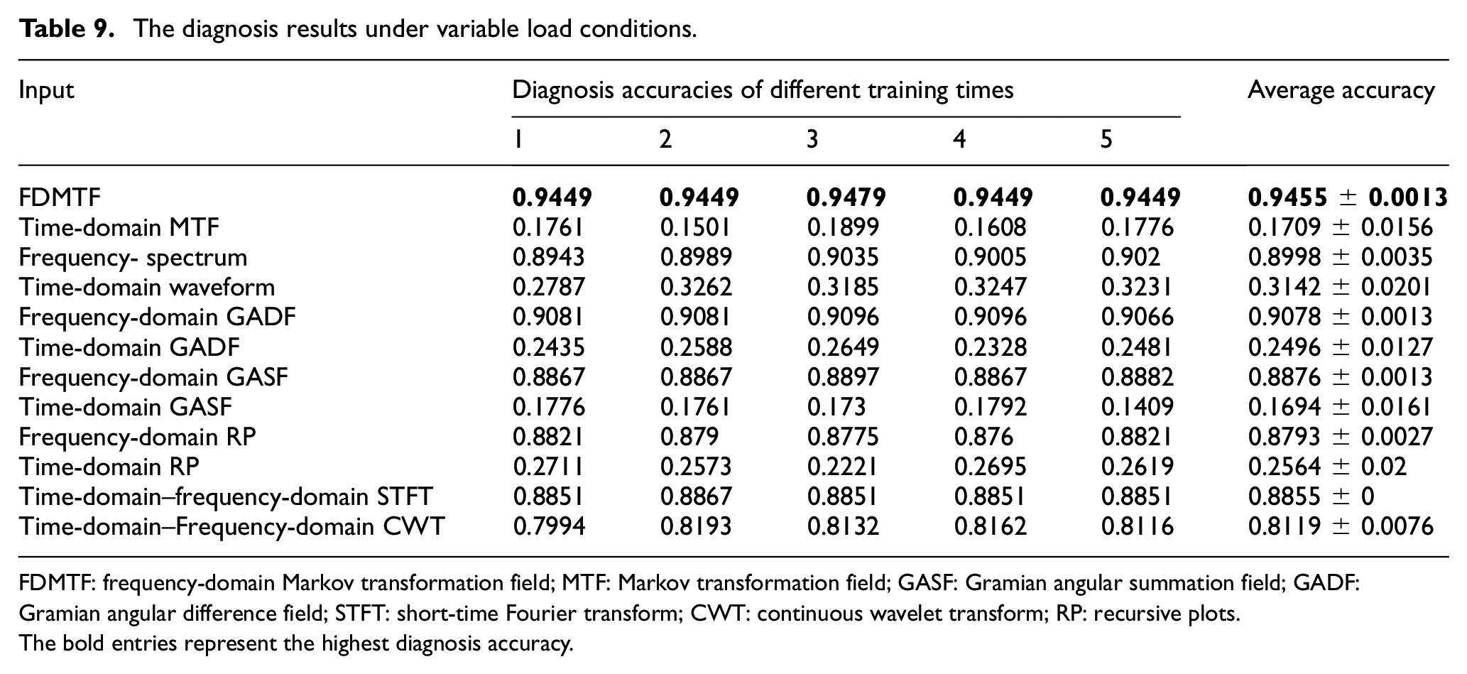
FDMTF: frequency-domain Markov transformation field; MTF: Markov transformation field; GASF: Gramian angular summation field; GADF: Gramian angular difference field; STFT: short-time Fourier transform; CWT: continuous wavelet transform; RP: recursive plots.The bold entries represent the highest diagnosis accuracy.

Table 9 shows the recognition accuracy under different loads when 12 different characterization methods are used as the input of MBRCNN. The recognition accuracy obtained by the FDMTF is the highest, which proves once again the superiority of FDMTF. Seven of the 12 characterization methods achieve recognition accuracy of more than 80% with a small standard deviation. The order of recognition accuracy of different inputs is FD based > time–frequency domain based > time-domain based.

Discussions

The robustness of the proposed method is reflected by its ability to resist changes in the following three aspects: the number of training samples, the network hyper-parameters and the variable load conditions. Tables 3 and 7 show that the recognition accuracy exceeds 95% in two cases under the training sets with different proportions, which shows the robustness of the proposed method against the number of training samples. Figure 14 shows that the average diagnosis accuracy exceeds 95% when the three hyper-parameters are changed in turn, which shows the robustness of the proposed method against the network hyper-parameters. The recognition accuracy of fault diagnosis under variable loads in Case 2 is 94.55%, which shows the robustness of the proposed method against variable loads.

Based on the UoC gearbox dataset, the recognition accuracy of the proposed method exceeds that of the seven state-of-the-art methods in Refs. 42–48, which shows its progressive significance. The diagnosis accuracy of Case 2 is lower than that of Case 1, which may be because the vibration signal of Case 2 is more complex and contains more noise interference.

In combination with Figures 8 and 9, it can be found that FDMTF can make the characterization of vibration signals of the same running status similar and the vibration signals of different running statuses different, which proves that it can be used as the input of CNN for identifying gearbox faults. In the two case studies, the samples participating in each health status training are some dozens, not thousands, and the recognition accuracy of more than 98.8% is still obtained. With only 10% training samples in Case 1, 100% recognition accuracy can still be achieved. In Case 2, when there are only 25% training samples, the recognition accuracy can reach 95.72%. It shows that the good representation of the 1D vibration signal provides a potential possibility for solving the small sample problem.

The original intention of the MBRCNN network structure is to extract the multiple scale features and avoid a series of problems caused by the deep network structure. Figure 14 shows that the proposed model is insensitive to hyper-parameters with the help of MB blocks and residual blocks. However, it should still be noted that to obtain high recognition accuracy, the learning rate may be worthy of attention. According to the analysis in Figure 14(c), a learning rate of about 0.001 is recommended.

The results in Table 5, 9 and Figure 11 show that the methods based on the time-domain signal are not suitable to characterize the vibration signal of the QCC gearbox. There are noise interferences in the QCC gearbox vibration signal,^52,53 which may bring great differences to the vibration signals even under the same health status. In addition, the signal characterization methods, such as GAF and MTF, are affected by the phase of the time series itself, which is proved by Bai et al.³² as well as this article. Therefore, the 2D image encoding method based on the FD signal is recommended to replace the time-domain signal.

Table 5 and Figure 11 show that the recognition accuracy obtained by time-domain MTF is the lowest among the 12 methods, lower than time-domain GAF and even lower than time-domain waveform. However, the recognition accuracy obtained by FDMTF is higher than that obtained by FDGAF. The mechanism is not clear, which is worthy of further research.

The recognition accuracy of FDGAF in Table 5 is more than 98%, which shows that it is also a good 2D image encoding method. In addition, it can be found that GADF is better than GASF in both encoding FD signals and time-domain signals. This result is consistent with the research results in Han et al.³¹, Zhang et al.⁵³ Although GASF has achieved satisfactory results in Tang et al.²⁹, Bai et al.³² for mechanical fault diagnosis, it is suggested that when using GAF for encoding the vibration signals, GADF instead of GASF can be considered.

Table 6 shows that using the network parameters trained by the ImageNet dataset to fine-tune the network parameters based on FDMTF data is not necessarily suitable. The reason is that there may be great differences between the two kinds of image data. The method of pre-training parameters shown in Table 6 also failed to achieve the expected results. If the network model parameters trained by FDMTF of vibration signals collected from other gearboxes can be used, pre-training as well as fine-tuning may be helpful to reduce training costs of the QCC gearbox fault diagnosis model.

Zhang et al.¹¹ used domain adaption technology to solve the problem that training data and testing data come from different load conditions. The seven methods of 2D characterization of vibration signals in Table 9 can achieve a recognition accuracy of more than 80%, including 94.55% obtained by the proposed method, which does not use domain adaptation or other transfer learning techniques. Similar to the research results obtained in Zhang et al.¹⁹ 2D image representation of vibration signals combined with CNN can provide a potential idea for fault diagnosis under variable load conditions.

Conclusion

To accurately identify QCC gearbox faults, this article proposes a method, namely, FDMTF–MBRCNN, which benefits FDMTF and MBRCNN. Compared with time-domain MTF, the FDMTF can ignore the difference caused by the signal phase and is more robust than MTF to background noise. MBRCNN combines the advantages of MB and residual blocks. The experimental data collected from the UoC gearbox and the QCC scaled-down test rig achieve diagnosis accuracy of 100% and 98.85%, respectively, which proves the availability of the proposed method. The recognition accuracy of more than 94% can be obtained under different proportions of training samples, hyper-parameter combinations or variable loads, which proves the robustness of the FDMTF–MBRCNN method. The specific conclusions are as follows:

A QCC gearbox fault diagnosis method integrating FDMTF and MBRCNN is proposed. Its effectiveness and superiority are proved by the two case analyses and the comparison with the other methods.

The FDMTF is used to encode 1D vibration signals into 2D images, whose recognition accuracy is higher than that of the other 11 methods. FDMTF is recommended for encoding the vibration signal rather than time-domain MTF. In addition, for fault diagnosis based on CNN, the 2D encoding method is recommended for FD signals instead of time-domain signals.

When using FDMTF as input, the MBRCNN can effectively extract the features of different signals, whose extraction ability and recognition accuracy are better than four methods, that is, ResNet-18 adopts three different training strategies as well as AlexNet.

The FDMTF–MBRCNN method has the potential capabilities to solve the small sample problem and the variable load problem, which have been the hot issues in the current fault diagnosis field.

Our future work will further focus on the research of 2D representation of vibration signals to realize QCC gearbox fault diagnosis under variable speed conditions.

Footnotes

Declaration of conflicting interests

The authors declared no potential conflicts of interest with respect to the research, authorship, and/or publication of this article.

Funding

The authors received no financial support for the research, authorship, and/or publication of this article.

ORCID iD

Qing Zhang

References

Feng

Chen

, et al. A cyclostationarity-based wear monitoring framework of spur gears in intelligent manufacturing systems. Struct Health Monit. Epub ahead of print 12 January 2023. DOI: 10.1177/14759217221147018.

Wang

. Degradation feature extraction of quay side crane lifting gearbox based on Katz fractal dimensional-Singular value decomposition. In: IEEE, 2021 4th world conference on mechanical engineering and intelligent manufacturing (WCMEIM), Shanghai, China, 12–14 November 2021, pp. 400–404. New York: IEEE.

Inturi

Balaji

Gyanam

, et al. An integrated condition monitoring scheme for health state identification of a multi-stage gearbox through Hurst exponent estimates. Struct Health Monit 2023; 22(1): 730–745.

Feng

A novel adaptive bandwidth selection method for Vold–Kalman filtering and its application in wind turbine planetary gearbox diagnostics. Struct Health Monit, 2022; 22(2): 1027–1048.

Pang

Tian

Tang

GJ.

Fault state recognition of wind turbine gearbox based on generalized multi-scale dynamic time warping. Struct Health Monit 2021; 20(6): 3007–3023.

Praveen

Jaikanth

Inturi

, et al. Fingerprinting based data abstraction technique for remaining useful life estimation in a multi-stage gearbox. Measurement 2021; 174: 109021.

Liu

Yang

Zio

, et al. Artificial intelligence for fault diagnosis of rotating machinery: a review. Mech Syst Signal Process 2018; 108: 33–47.

Buckley

Ghosh

Pakrashi

A feature extraction & selection benchmark for structural health monitoring. Struct Health Monit. Epub ahead of print 9 September 2022. DOI: 10.1177/1475921722111114.

Zhang

Zhong

, et al. A GOA-MSVM based strategy to achieve high fault identification accuracy for rotating machinery under different load conditions. Measurement 2020; 163: 108067.

10.

Fan

Jia

, et al. Research on multi-domain fault diagnosis of gearbox of wind turbine based on adaptive variational mode decomposition and extreme learning machine algorithms. Energies 2020; 13(6): 1–20.

11.

Zhang

Qin

, et al. An intelligent fault diagnosis method based on domain adaptation for rolling bearings under variable load conditions. Proc IMechE, Part C: J Mechanical Engineering Science 2021; 235(24): 8025–8038.

12.

Lei

Jia

Lin

, et al. An intelligent fault diagnosis method using unsupervised feature learning towards mechanical big data. IEEE Trans Ind Electron 2016; 63(5): 3137–3147.

13.

Yang

Fault diagnosis of rolling bearings using an improved multi-scale convolutional neural network with feature attention mechanism. ISA Trans 2021; 110: 379–393.

14.

Zhang

Huang

, et al. Multi-model ensemble deep learning method for intelligent fault diagnosis with high-dimensional samples. Front Mech Eng 2021; 16(2): 340–352.

15.

Liu

Knowledge extraction and insertion to deep belief network for gearbox fault diagnosis. Knowl-Based Syst 2020; 197(10583): 1–13.

16.

Wang

An intelligent diagnosis scheme based on generative adversarial learning deep neural networks and its application to planetary gearbox fault pattern recognition. Neurocomputing 2018; 310: 213–222.

17.

Jiang

Shao

, et al. Intelligent fault diagnosis of rolling bearings using an improved deep recurrent neural network. Meas Sci Technol 2018; 29(0651107): 1–15.

18.

Janssens

Slavkovikj

Vervisch

, et al. Convolutional neural network based fault detection for rotating machinery. J Sound Vib 2016; 377: 331–345.

19.

Zhang

Wang

, et al. An FSK-MBCNN based method for compound fault diagnosis in wind turbine gearboxes. Measurement 2021; 172(6): 108933.

20.

Ding

Energy-fluctuated multiscale feature learning with deep ConvNet for intelligent spindle bearing fault diagnosis. IEEE Trans Instrum Meas 2017; 66(8): 1926–1935.

21.

Bai

Yang

Wang

, et al. Image representation of vibration signals and its application in intelligent compound fault diagnosis in railway vehicle wheelset-axlebox assemblies. Mech Syst Signal Process 2021; 152: 10471.

22.

Khodja

Guersi

Saadi

, et al. Rolling element bearing fault diagnosis for rotating machinery using vibration spectrum imaging and convolutional neural networks. Int J Adv Manuf Technol 2020; 106: 1737–1751.

23.

Wang

Zhao

, et al. Motor fault diagnosis based on short-time fourier transform and convolutional neural network. Chin J Mech Eng 2017; 30(6): 1357–1368.

24.

Cheng

Lin

, et al. Intelligent fault diagnosis of rotating machinery based on continuous wavelet transform-local binary convolutional neural network. Knowl-Based Syst 2021; 216(1): 106796.

25.

Hatami

Gavet

Debayle

. Classification of time-series images using deep convolutional neural networks. In: Tenth international conference on machine vision (ICMV), Vienna, Austria, 2017, pp. 1–8.

26.

Wang

Oates

Imaging time-series to improve classification and imputation. In: Proceedings of the twenty-fourth international joint conference on artificial intelligence (IJCAI), Buenos Aires, Argentina, 2015, pp. 3939–3945. Washington, D. C.: AAAI Press.

27.

Wang

Oates

Encoding time series as images for visual inspection and classification using tiled convolutional neural networks. In: Workshops at the twenty-ninth AAAI conference on artificial intelligence, Austin, YX, USA, 2015.

28.

Hsueh

Ittangihala

, et al. Condition monitor system for rotation machine by CNN with recurrence plot. Energies 2019; 12(17): 3221.

29.

Tang

Liao

Chen

, et al. A novel convolutional neural network for low-speed structural fault diagnosis under different operating condition and its understanding via visualization. IEEE Trans Instrum Meas 2021; 70: 1–11.

30.

Yang

, et al. A data-driven adaptive fault diagnosis methodology for nuclear power systems based on NSGAII-CNN. Ann Nucl Energy 2021; 159: 108326.

31.

Han

Zhang

Sun

, et al. A new bearing fault diagnosis method based on capsule network and Markov transition field/Gramian angular field. Sensors 2021; 21(22): 7762.

32.

Bai

Yang

Wang

, et al. Intelligent diagnosis for railway wheel flat using frequency-domain Gramian angular field and transfer learning network. IEEE Access 2020; 8: 105118–105126.

33.

Krizhevsky

Sutskever

Hinton

GE.

Imagenet classification with deep convolutional neural networks. Communications of the ACM 2017; 60(6): 84–90. Adv Neural Inf Process Syst 2012: 1097–1105.

34.

Szegedy

Liu

Jia

, et al. Going deeper with convolutions. In: 2015 IEEE conference on computer vision and pattern recognition (CVPR), 7–12 June 2015, Boston, MA, USA, 2015, pp. 1–9. New York, NY: IEEE.

35.

Zhang

Ren

, et al. Deep residual learning for image recognition. In: 2016 IEEE conference on computer vision and pattern recognition (CVPR), 27–30 June 2016, Las Vegas, NV, USA, 2016, pp. 770–778. New York, NY: IEEE.

36.

Jin

Ren

, et al. A multi-perspective architecture for high-speed train fault diagnosis based on variational mode decomposition and enhanced multi-scale structure. Appl Intell 2019; 49(11): 3923–3937.

37.

Zhang

Tang

Deng

, et al. A hybrid attention improved ResNet based fault diagnosis method of wind turbines gearbox. Measurement 2021; 179(10): 109491.

38.

Kingma

. Adam: a method for stochastic optimization. arXiv:1412.6980, 2014. Doi: 10.48550/arXiv.1412.6980

39.

Cao

Zhang

Tang

Preprocessing-free gear fault diagnosis using small datasets with deep convolutional neural network-based transfer learning. IEEE Access 2018; 6: 26241–26253.

40.

Cao

Zhang

Tang

Gear Fault Data. https://doi.org/10.6084/m9.figshare.6127874.v1 (2018, accessed 9 December 2021).

41.

Zhao

, et al. Deep learning algorithms for rotating machinery intelligent diagnosis: an open source benchmark study. ISA Trans 2020; 107: 224–255.

42.

Jin

Hou

Chen

A time series transformer based method for the rotating machinery fault diagnosis. Neurocomputing 2022; 494: 379–395.

43.

Ruan

, et al. An optimized stacked diagnosis structure for fault diagnosis of wind turbine planetary gearbox. Meas Sci Technol 2021; 32(7): 075102.

44.

Qian

Liu

Development of deep reinforcement learning-based fault diagnosis method for rotating machinery in nuclear power plants. Prog Nucl Energy 2022; 152: 104401.

45.

Qian

Liu

Fault diagnosis based on conditional generative adversarial networks in nuclear power plants. Ann Nucl Energy 2022; 176: 109267.

46.

Cao

Chen

, et al. Task-incremental broad learning system for multi-component intelligent fault diagnosis of machinery. Knowl-Based Syst 2022; 246: 108730.

47.

Qin

, et al. Machinery fault diagnosis scheme using redefined dimensionless indicators and mRMR feature selection. IEEE Access 2020; 8: 40313–40326.

48.

Shao

Xia

Wan

, et al. Modified stacked autoencoder using adaptive morlet wavelet for intelligent fault diagnosis of rotating machinery. IEEE/ASME Trans Mechatron 2021; 27(1): 24–33.

49.

Maaten

LVD

Hinton

. Visualizing data using t-SNE. J Mach Learn Res 2008; 9(2605): 2579–2605.

50.

Zhang

, et al. Fault diagnosis for small samples based on attention mechanism. Measurement 2022; 187: 110242.

51.

Deng

Dong

Socher

, et al. ImageNet: a large-scale hierarchical image database. In: 2009 IEEE conference on computer vision and pattern recognition (CVPR), 20–25 June 2009, Miami, FL, USA, 2009, pp. 248–255. New York, NY: IEEE.

52.

Zhang

Qin

, et al. A two-stage fault diagnosis methodology for rotating machinery combining optimized support vector data description and optimized support vector machine. Measurement 2022; 200: 111651.

53.

Zhang

Feng

, et al. Gearbox fault diagnosis based on frequency-domain Gramian angular difference field and deep convolutional neural network. Proc IMechE, Part C: J Mechanical Engineering Science 2023. Epub ahead of 3 March 2023. DOI: 10.1177/09544062231157189.

Robust fault diagnosis of quayside container crane gearbox based on 2D image representation in frequency domain and CNN

Abstract

Keywords

Introduction

The frequency-domain MTF

Markov transformation field

The proposed FDMTF

The proposed fault diagnosis method

The constructed CNN model

The steps of the FDMTF–MBRCNN method

Case study

Case 1: UoC gearbox dataset

Comparison analysis of Case 1

Case 2: QCC gearbox dataset

Comparison analysis of Case 2

The comparison with FDMTF

The comparison with MBRCNN

Robustness analysis based on Case 2

Robustness against proportions of training sample

Robustness against hyper-parameters

Robustness against variable loads

Discussions

Conclusion

Footnotes

Declaration of conflicting interests

Funding

ORCID iD

References