Deep learning-based concrete defects classification and detection using semantic segmentation

Abstract

Visual damage detection of infrastructure using deep learning (DL)-based computational approaches can facilitate a potential solution to reduce subjectivity yet increase the accuracy of the damage diagnoses and accessibility in a structural health monitoring (SHM) system. However, despite remarkable advances with DL-based SHM, the most significant challenges to achieving the real-time implication are the limited available defects image databases and the selection of DL networks depth. To address these challenges, this research has created a diverse dataset with concrete crack (4087) and spalling (1100) images and used it for damage condition assessment by applying convolutional neural network (CNN) algorithms. CNN-classifier models are used to identify different types of defects and semantic segmentation for labeling the defect patterns within an image. Three CNN-based models—Visual Geometry Group (VGG)19, ResNet50, and InceptionV3 are incorporated as CNN-classifiers. For semantic segmentation, two encoder-decoder models, U-Net and pyramid scene parsing network architecture are developed based on four backbone models, including VGG19, ResNet50, InceptionV3, and EfficientNetB3. The CNN-classifier models are analyzed on two optimizers—stochastic gradient descent (SGD), root mean square propagation (RMSprop), and learning rates—0.1, 0.001, and 0.0001. However, the CNN-segmentation models are analyzed for SGD and adaptive moment estimation, trained with three different learning rates—0.1, 0.01, and 0.0001, and evaluated based on accuracy, intersection over union, precision, recall, and F1-score. InceptionV3 achieves the best performance for defects classification with an accuracy of 91.98% using the RMSprop optimizer. For crack segmentation, EfficientNetB3-based U-Net, and for spalling segmentation, IncenptionV3-based U-Net model outperformed all other algorithms, with an F1-score of 95.66 and 89.43%, respectively.

Introduction

In structural health monitoring and condition assessment, deterioration detection and forecast are fundamental aspects. ¹ Civil infrastructures, including buildings, bridges, power-station, dams, and so on are essential parts of society, and most of these structures are made of concrete. However, these concrete structures deteriorate progressively due to the influence of extreme weather conditions, overloading, and lack of periodic maintenance. ² Eventually, concrete damages affect the structures’ safety, durability, and service life. ³ According to Yamane and Chun, ⁴ carbonation and chloride-induced corrosion are two prime components of the deterioration of reinforced concrete, and these components are usually induced through cracking and spalling. Thus, periodic visual inspection and early detection are vital in maintaining infrastructures. Traditionally, human-based inspections and analysis are considered for quantitative defects evaluation and foreseeing the restoration procedure. ⁵ However, these conventional methods are time-consuming, expensive, and highly dependent on the expertise of the investigators.^6,7 To solve these drawbacks, infrastructure owners have focused on developing various smart and autonomous damage assessment systems.^8–10

Considering the efficiency of vision-based monitoring methods, researchers have widely studied the unique features of these approaches over the decades. Primarily various image processing techniques (IPTs) were adopted to detect a few structural damages, such as cracks,^11,12 and spalling. ¹³ Despite being effective in detecting some specific image patterns, the robustness of IPTs is substantially affected when the images contain noises from lightning, shadows, and distortion. ¹⁴ In search of improved adaptability for damage assessment, the advent of artificial intelligence-based computer-vision methods have shown a remarkable appraisal.^15,16 Machine learning (ML)-based damage detection was initially used by Amezquita-Sanchez and Adeli ¹⁷ and Butcher et al. ⁸ to extract the features from an image. Later, an artificial neural network, a supervised ML method, was incorporated to enhance the efficiency of the different structural damage detection methods.^18,19 Even though ML methods’ performance has been relatively decent, the 2012 introduction of convolutional neural network (CNN) gave a robust solution for object recognition and classification. ¹⁵ A CNN-based deep learning (DL) method was developed to detect concrete cracks by Cha et al. ²⁰ and Pan and Yang ²¹ and other defects by Lin et al. ²² The CNN model has different algorithms based on the depth and width of the learning layers. Researchers are continuously exploring pre-built and own-developed CNN algorithms to develop an effective damage assessment model. Among all the pre-built base models, Visual Geometry Group (VGG)Net, ²³ Residual Network (ResNet), ²⁴ and Inception ²⁵ models are highly recognized for damage pattern recognition and detection process. VGGNet-built in 2014 by VGG from Oxford University, used 3 × 3 convolutional filters with 16 and 19 convolutional layers and achieved an outstanding performance without having too deep layers. However, VGGNet faced a vanishing gradient problem where the learning rate became smaller within the deeper layer, increasing the training time considerably. In 2015, researchers proposed ResNet to solve the vanishing gradient issue. ResNet uses the “skip connection” concept within the residual block, allowing the gradient an alternate shortcut without hindering the performance of the deeper layers. In 2014, in the ImageNet visual recognition competition, the Inception model put forward a breakthrough performance to solve recognition and detection problems. The objective of the Inception model was to increase the depth and width of the model while avoiding overfitting and extensive computational cost. To upgrade the damage evaluation process, researchers have worked on developing their own CNN model while using the pre-built base models as the backbone of the structure. In recent years, DeepCrack, ²⁶ SDDNet, ²⁷ STRNet, ²⁸ and U-Net ²⁹ have gained popularity over the base models with their robust performance in crack detection. The aforementioned studies found that these models were successful in crack detection with a performance evaluation matric intersection over union (IoU) value of 0.88, 0,846, 0.926, and 0.923 for DeepCrack, SDDNet, STRNet, and U-Net, respectively.

Conventionally, CNN-based damage detection can be categorized into three sections-—image patch method, boundary box regression, and semantic segmentation. ³⁰ Image patch method uses small patches to identify the damage on the image (Figure 1(a)). For the boundary box regression method, the model uses a box to bound the area of the damage (Figure 1(b)). Pan and Yang ²¹ adopted CNN method with the image patch technique and Feng et al. ³¹ and Xue and Li ³² applied CNN to localize the damages on the images. Subsequently, region-based CNN models (R-CNN) were proposed by a few researchers, with simple modifications for multiple damage detection, like—Faster R-CNN.^32–36 In another study, Cha et al. ³⁷ used Faster R-CNN to detect five defects—concrete crack, steel corrosion, bolt corrosion, and steel delamination. Nevertheless, the image patch method and R-CNN were incapable of extracting the exact geometry of the damages as it worked by dividing the images into patches and boxes, respectively. However, pixel-wise analysis using CNN-based semantic segmentation can get a more quantitative assessment of damage characteristics (Figure 1(c)), and this study has used this approach for damage detection. A detailed review of CNN-based semantic segmentation with various application techniques was presented in the study by Garcia-Garcia et al. ³⁸ Liu et al. ¹⁵ proposed U-Net architecture to build an autonomous pavement crack segmentation model. ResNet34 was applied as the backbone base model, which was pretrained by ImageNet parameters. The proposed segmentation model detected cracks with precision, recall, and F1-score of 97.24, 94.31, and 95.75%, respectively. Recently, FCN-based CNN algorithms have been extensively analyzed for semantic segmentation. ³ FCNs are implemented as an end-to-end pixel-level process where the final outcome is semantic segmentation instead of damage categorization.

Figure 1.

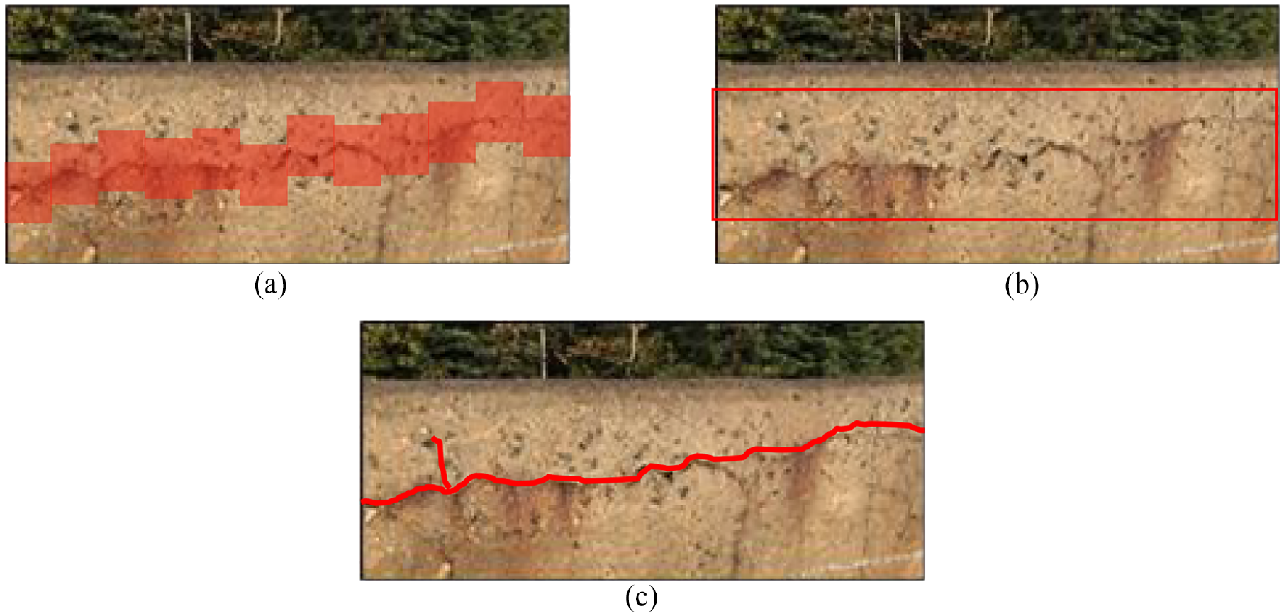
Defect detection with (a) image patch classification, (b) boundary box regression, and (c) semantic segmentation.

Designing a new CNN model by accounting for the relevant parts of a pretrained model is named transfer learning in DL. After analyzing the existing literature, it has been found that transfer learning is extensively used in vision-based investigation, as it has shown promising results in damage detection with a lower computational cost. VGGNet, ResNet, and MobileNet are the three most prevalent base models used as the backbone for damage detection using CNN models. Despite these notable achievements, some unexplored issues in concrete damage assessment include considering one specific type of damage-crack. In contrast, DL methods are well-known for multi-class classifiers. Moreover, most past studies used datasets developed with defect-targeted images, missing realistic environmental exposures. Additionally, most past studies explored the semantic segmentation detection process with one or two models, eluding the defects categorization, while a comprehensive damage assessment requires both. After exploring the existing studies, this study aimed to develop a CNN-based algorithm for damage detection and classification of concrete structures. First, a diverse dataset is developed with real images from field inspection reports and available online resources that include various background noises replicating actual field conditions to achieve this objective. This study considers two different concrete damages, cracking and spalling. After that, three different models, VGG19, ResNet50, and InceptionV3, are considered for damage classification. The sensitivity analysis of defects classification is done on two optimization functions—stochastic gradient descent (SGD) and root mean square propagation (RMSprop), with a learning rate of 0.1, 0.001, and 0.0001. For semantic segmentation, two encoder-decoder models, U-Net and pyramid scene parsing network (PSP-Net), are used where VGG16, ResNet50, InceptionV3, and EfficientNetB3 CNN models are considered as backbone base models. Finally, all the segmentation models are analyzed with two optimization functions—SGD and adaptive moment estimation (ADAM) and three learning rates 0.1, 0.01, and 0.0001, and evaluated based on accuracy, IoU, precision, recall, and F1-score. Encoder-decoder model is still a new concept for multiple defects segmentation. To the authors’ knowledge, no previous studies were conducted for concrete crack and spalling area detection using U-Net and PSP-Net architecture-based encoder-decoder models. Also, this study has used U-Net and PSP-Net architecture with four backbone models, including InceptionV3 and EfficientNetB3. No previous studies used these two backbone models for concrete spalling detection.

Research method

This study is conducted in two steps—first, multi-class damage classification and then damage area detection using semantic segmentation. As shown in Figure 2, the overall process for both cases starts with image acquisition for concrete cracks and spalling from available online resources and inspection reports, followed by processing the images into the desired resolution. Then, the whole dataset is randomly split into training, validation, and testing datasets for data preparation. After finalizing the datasets comes the adoption and implementation of different CNN models. Multiple CNN-based models are used for classification and segmentation, such as—VGG16, ResNet50, InceptionV3, and EfficientNetB3.

Figure 2.

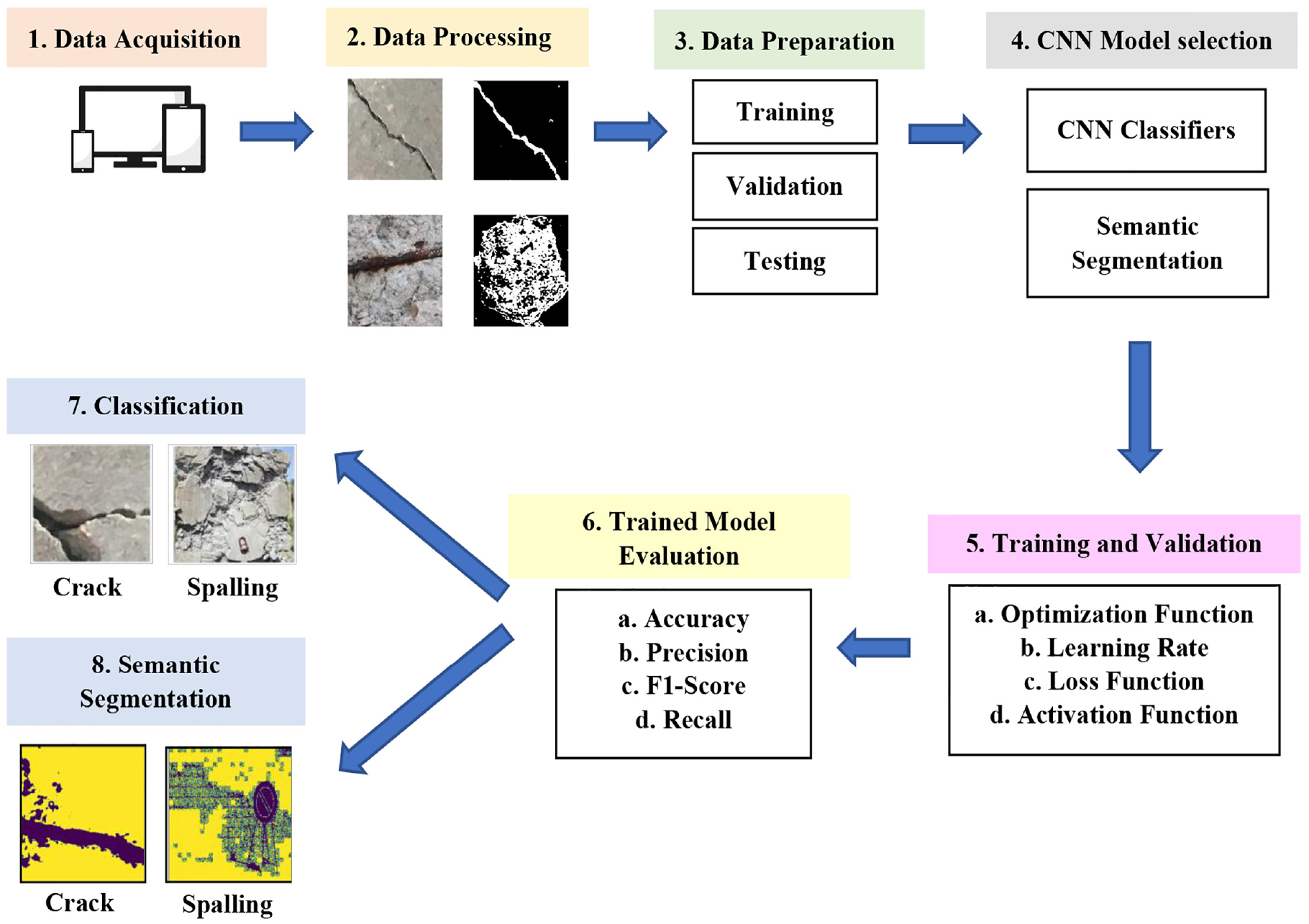
Overall process of proposed defects identification and condition assessment model.

For training and validation, the models use optimization, learning rate, loss, and activation functions to tune the hyper-parameters to achieve a better training performance. Hyper-parameters are the parameters that control the training process to achieve the optimization point of the model. Later the trained model is evaluated based on four different evaluation metrics—accuracy, precision, F1-score, and recall. Finally, the testing dataset is used to predict defects classification and segmentation. In the segmentation process, two encoder-decoder models (U-Net and PSP-Net) are used to detect the image’s defect area. In contrast, the classification model uses a classifier function, softmax, to categorize the defects.

Optimization function and loss function

The optimization technique in a neural network works as finding the minimum or maximum output of the function depending on the input parameters or arguments. While updating the weights during the training process, the model minimizes the loss function and optimizes the prediction performance. The loss function guides the optimizers by quantifying the difference between the expected result and the predicted result of the model. For this study, two optimizers are used—SGD and ADAM.

SGD is a process linked with a random probability. Here, a single random image is taken for each iteration. SGD uses a single sample to find the gradient of the loss function rather than using the summation of the loss function of all the samples. RMSprop has a special feature which restrains the swaying in the vertical direction when helping the learning rate to learn faster in the horizontal direction, making the converging faster. ADAM is a gradient descent optimizer that includes two types of gradient descent—Momentum and RMSprop algorithm, which is very efficient and requires very little memory. ³⁹ Momentum helps speed up the gradient descent of the network by taking the exponentially weighted average. RMSP also accelerates the optimization process by reducing the number of function evaluations. This optimizer is formulated by taking the average of weights squared gradients and dividing by the square root of the mean square.

Activation function

In a neural network, the activation layer uses an activation function (nonlinear) to navigate how the weighted sum of the input transforms from nodes to output. In this study, Rectified Linear Activation (ReLu) function (Figure 3) is used for all the CNN models and shown in Equation (1). This ReLu activation function f () can be described mathematically using the max () function over the set of 0 and the input z.

$$f\left(z\right)=\max (0,z)$$

(1)

Figure 3.

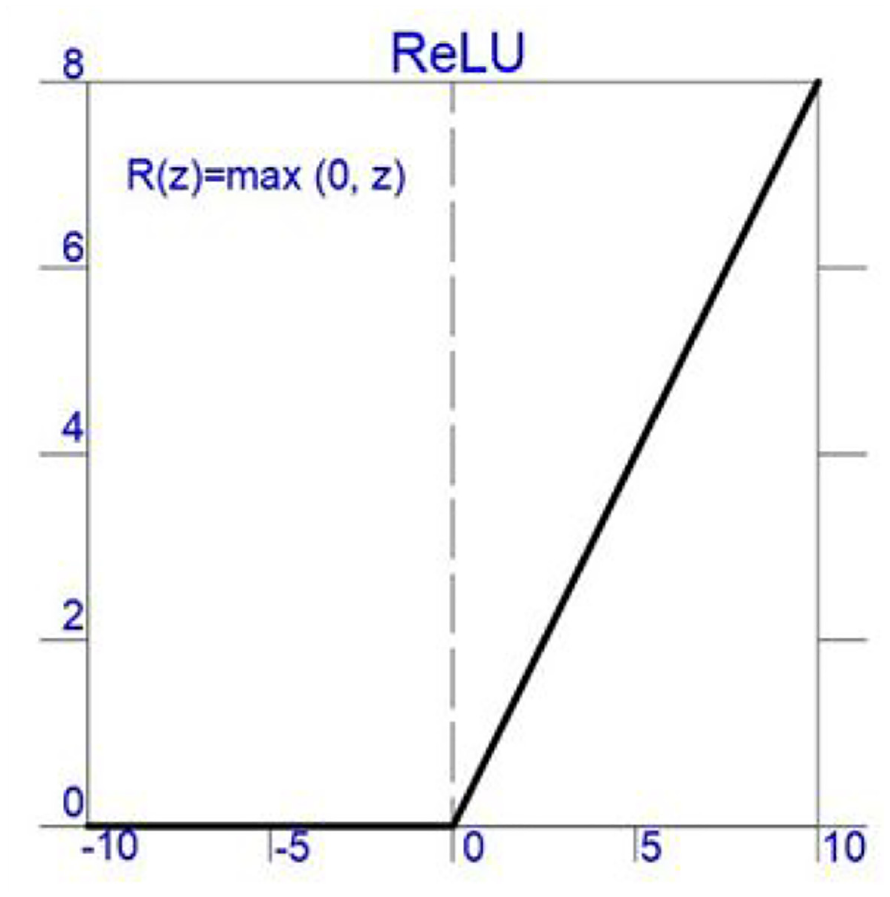
Activation function (ReLu).

Softmax layer

The smooth approximation of the argument max function, Softmax, is an activation function implied in the output layer of the neural network model, which predicts the multi-nominal probability distribution and acts as a multi-class classification layer. The softmax function allocates a decimal probability to each class, adding up to 1. Equation (2) denotes the formulation of the softmax layer.

$$\mathrm{softmax}\left(z_i\right)=\frac{\exp \left(z_i\right)}{{\sum }_j\exp \left(z_j\right)}$$

(2)

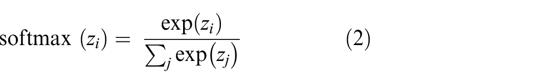
Here z denotes the values from the output layer. The exponential function represents the nonlinear function. The summation of the exponential value in the formula works as the normalization term, ensuring that the function’s output values will sum to 1.

Data preparation

Data collection

One of the main aspects to guarantee CNN models’ robust performance is developing an organized dataset. For achieving significant performance with the CNN model, a dataset should consist of high-quality images with various noises, replicating the real-time environmental conditions, such as surface roughness, background debris, lighting conditions, shadow, and so on. As mentioned by Zhang et al., ⁴⁰ the DL model’s performance severely relies on the quality and quantity of the dataset and is highly affected by low-quality images. Moreover, studies have observed that DL methods can perform better with a monotonous image background. Still, accuracy can easily drop when a prediction is made on an image with a complex background. For example, Choi and Cha ²⁷ observed that when a CNN model is trained with targeted images of noise-free background and subsequently tested on images with rough background, the performance accuracy drastically declined, dropping the precision from 0.874 to 0.231.

This study has focused on developing a dataset using real-world structural inspection reports to collect images with rough backgrounds to comply with the aforementioned statement. However, due to the shortage of images from inspection reports, this study has also taken advantage of the online resources. Crack and spalling images are retrieved from a freely available annotated open dataset, ⁴¹ inspection reports of concrete structures obtained from local industries, and available damage images from various experimental tests on concrete members. The annotation is done manually for the images from the inspection reports. The resulting crack and spalling datasets have 4087 and 1100 images, respectively. The entire dataset is pixel-based, presenting one single defect per image. Therefore, it is improbable to have a crack and spalling close by in practical conditions. A few sample photos of concrete crack and spalling are presented in Figure 4.

Figure 4.

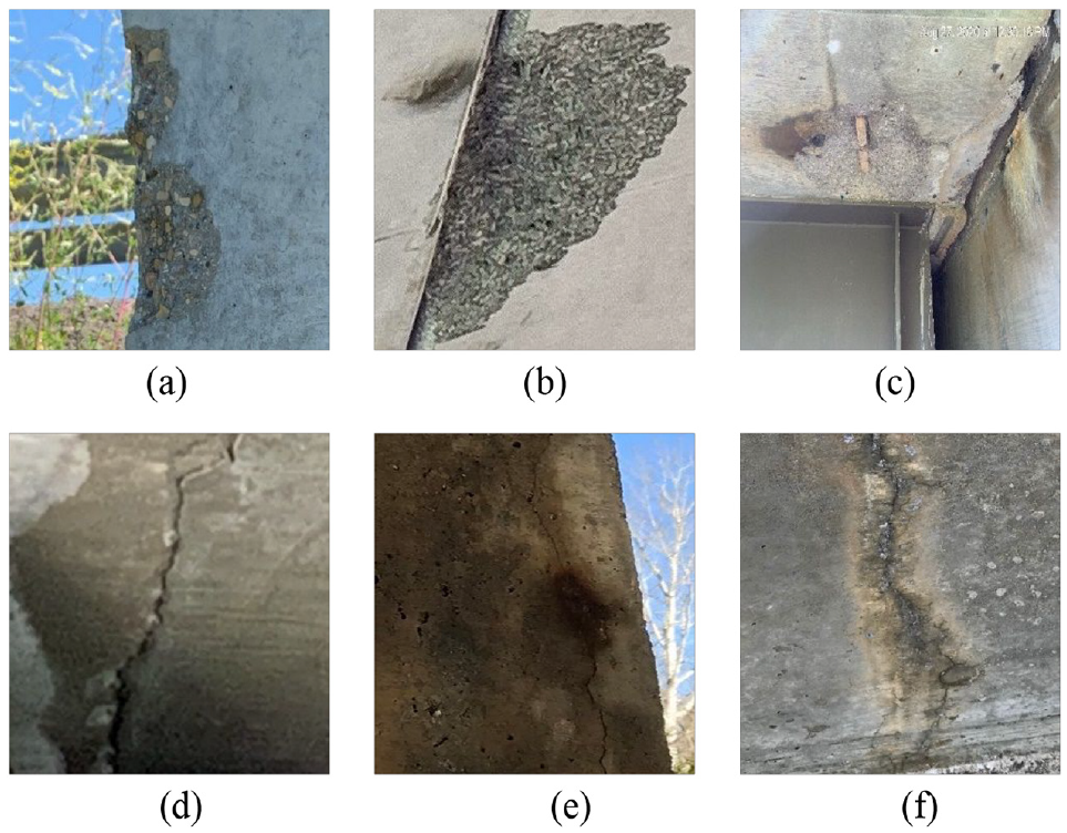
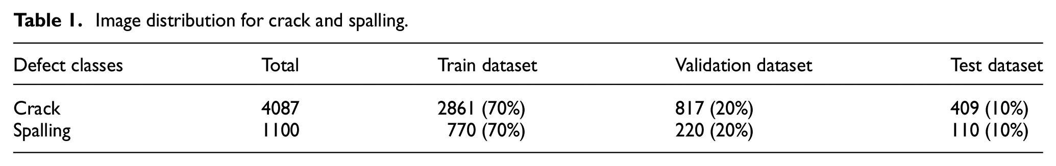
Sample images for defects dataset (a, b, and c) spalling and (d, e, and f) crack.

Data processing

The dataset contains images of various resolutions as the defects images are collected from multiple sources. To standardize the image format for DL analysis, images are converted into a resolution of 224 × 224 pixels with red-green-blue (RGB) channels for both the classifier and semantic segmentation CNN models. As suggested in a previous study, when the DL model is trained using images with comparatively small pixels, the model can learn the desired features more precisely. ⁴² The developed dataset considers various crack and spalling image resolutions and dimensions. Different areas, lengths, widths, and shapes, including vertical, horizontal, and zigzag on various concrete surfaces, are studied for both cracks and spalling. For a proper model generation, the dataset must be utilized properly as training, validation, and testing dataset. In general, an 80–20% train-test split is adopted by many researchers. For instance, Wang et al., ⁴³ Li and Zhao, ⁴⁴ and Yang et al. ⁴⁵ used 80% of the dataset for training and validation and 20% as the testing subset. However, there is no universal approach for dataset division, as some researchers have used 70 and 60% of the whole dataset for training and validation and the rest of the 30 and 40% for the testing purpose, respectively.^46,47 The entire dataset is randomly split into 70–20–10% for training, validation, and testing in this study for both classification and segmentation cases. Table 1 presents the distribution of images used for training, validation, and testing. A ground truth mask dataset is created for semantic segmentation using the original 224 × 224 pixel images. Ground truth refers to the location of the exact features on an image, which helps the model measure the features more accurately. The threshold method is implemented to develop the ground truth dataset. The threshold is an image-processing technique that separates the object from the background pixels.

Table 1.

Image distribution for crack and spalling.

Defect classes	Total	Train dataset	Validation dataset	Test dataset
Crack	4087	2861 (70%)	817 (20%)	409 (10%)
Spalling	1100	770 (70%)	220 (20%)	110 (10%)

Transfer learning

For defects classification and semantic segmentation, transfer learning is an important criterion for weight training initialization and fine-tuning. Transfer learning refers to reutilizing a pre-developed CNN model to develop other related models. Typically, initializing a new CNN model’s training requires a large amount of data, and transfer learning can reduce the size of the trainable parameters. But, to successfully use the transfer learning from the pretrained model, the model needs to be pretrained with a large amount of data. ⁴⁸ There are two methods for transfer learning—(a) feature extraction and (b) fine-tuning. In the first method, the existing pre-built network works as a feature extractor to learn the features from the input images. Then the trained features are implemented in the new model for training purposes. In the latter method, the pretrained hyper-parameters are used for training a new dataset, and with every iteration, the new model learns with the help of the loss function and optimization function. Table 2 shows the details of the hyper-parameters used in this study.

Table 2.

Details of hyper-parameters.

Name of parameters	Value of parameters
Batch size (CNN-classifiers)	10
Batch size (CNN-segmentation)	10
Learning rate (CNN-classifiers)	0.1, 0.001, 0.0001
Learning rate (CNN-segmentation)	0.1, 0.01, 0.0001
Optimizers (CNN-classifier)	SGD, RMSprop
Optimizers (CNN-segmentation)	SGD, ADAM
Activation function	ReLu
Evaluation metrics threshold	0.5
Loss function (CNN-classifiers)	Binary cross-entropy
Loss function (CNN-segmentation)	Focal dice loss
Pretrained weights	ImageNet
Callbacks	Early stopping, reducinglearning rate

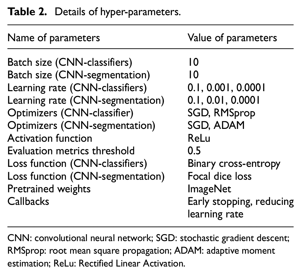
CNN: convolutional neural network; SGD: stochastic gradient descent; RMSprop: root mean square propagation; ADAM: adaptive moment estimation; ReLu: Rectified Linear Activation.

Semantic segmentation

For defects localization, this study considered the semantic segmentation process. In the semantic segmentation process, first, the objects are identified individually by assigning a class label to each pixel and later on, a segmentation mask is created for the same pixel values to locate the different objects from an image. Figure 5 shows a general overview of the semantic segmentation process where “1” indicates defects (i.e., crack) and “0” indicates background. According to Xing et al., ⁴⁹ encoder-decoder models are frequently used for the semantic segmentation process. In encoder-decoder model, the encoder part works on extracting the features and patterns of objects from an image, whereas the decoder part predicts the specific class of objects based on the trained features. In this study, two types of encoder-decoder models are considered—(a) U-Net and (b) PSP-Net.

Figure 5.

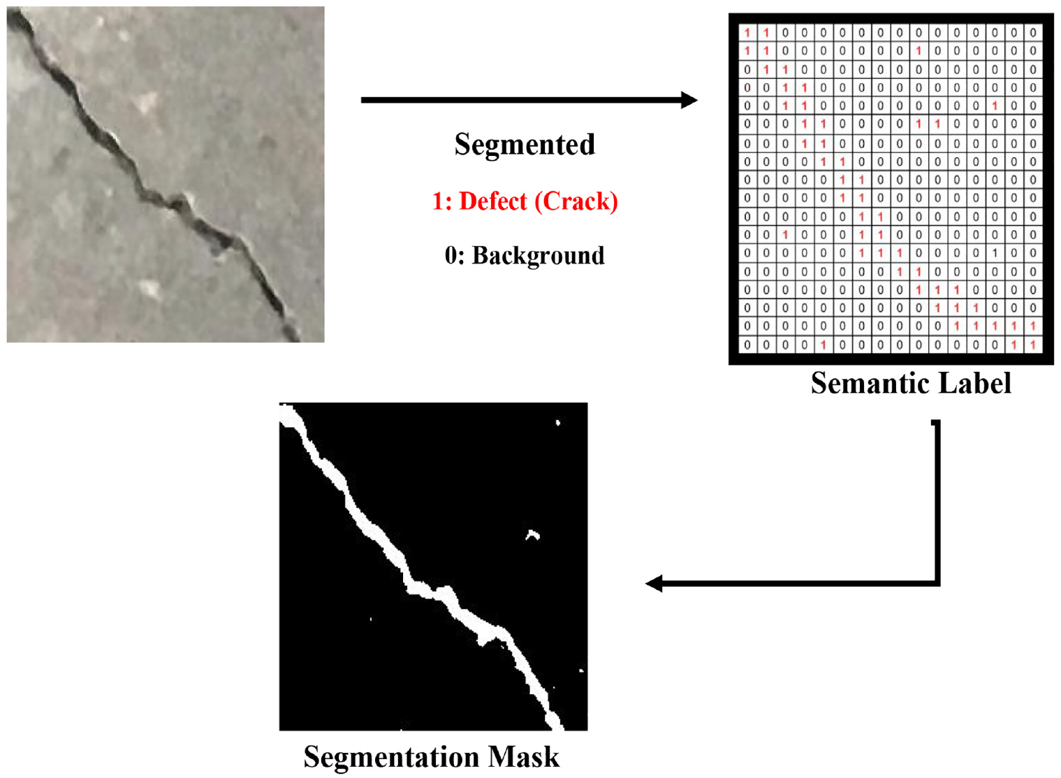
Schematic diagram of semantic image segmentation process.

U-Net architecture

U-Net ²⁹ is an encoder-decoder model which has a network architecture shape of “U” (Figure 6). The encoder component analyzes an input image through convolutional, activation, and pooling layers to learn different feature maps from the image. During this encoding process, the feature map reduces its size by losing the background information until the bottleneck segment of the U-Net. The encoder section starts with two repeated blocks of 3 × 3 convolutional layers followed by activation layer ReLu and batch normalization. These layers are named ConvBlock and come with a 2 × 2 max-pooling layer with a two-stride size, which helps downsample the image’s dimension. For the encoder network, four pretrained backbone models are considered—VGG19, ResNet50, InceptionV3, and EfficientNetB3 (Figure 7).

Figure 6.

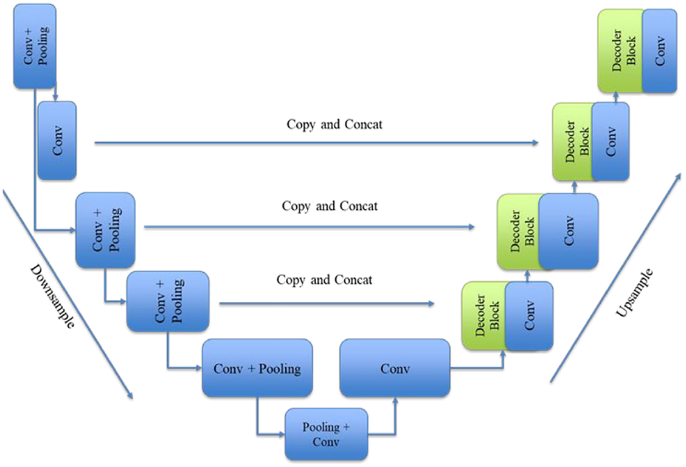
Schematic diagram of U-Net architecture.

Figure 7.

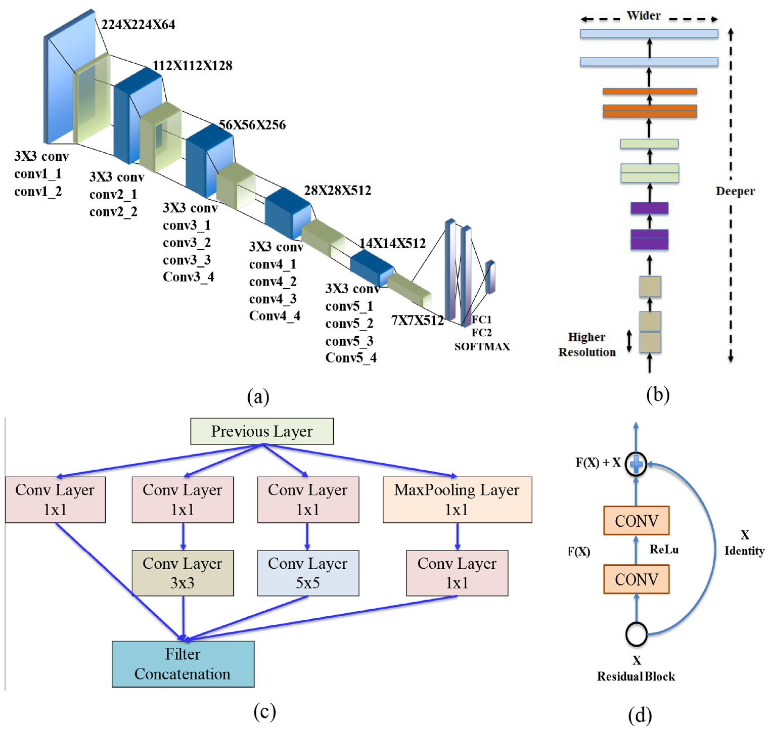
CNN base model architecture (a) VGG19, (b) EfficientNetB3, (c) InceptionV3, and (d) ResNet50.

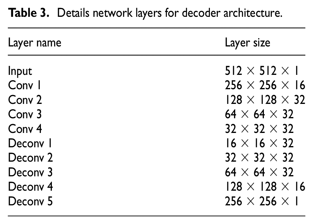
After the encoding part trains on recognizing the patterns from the image, the decoder part aims to recover the lost feature maps of the image. Here the model first encodes a 1/6 feature map from the ground truth image and then decodes a 1/6 feature map from the previous encoder part to make a segmentation prediction. Later, a 4 × 4 transpose convolutional layer is infused to increase the size of the image dimension. This model used a 3 × 3 convolutional layer for concatenation and a 1 × 1 convolutional layer for final detection. Table 3 shows the detailed network specification for the decoder architecture.

Table 3.

Details network layers for decoder architecture.

Layer name	Layer size
Input	512 × 512 × 1
Conv 1	256 × 256 × 16
Conv 2	128 × 128 × 32
Conv 3	64 × 64 × 32
Conv 4	32 × 32 × 32
Deconv 1	16 × 16 × 32
Deconv 2	32 × 32 × 32
Deconv 3	64 × 64 × 32
Deconv 4	128 × 128 × 16
Deconv 5	256 × 256 × 1

PSP-Net architecture

The semantic segmentation process uses the scene parsing technique, where the model assigns a unique class to each pixel while trying to understand the image. PSP-Net uses the scene parsing technique to predict the label of an object and recognize the geometrical parameters, that is, location and shape of the object. According to Zhao et al., ⁵⁰ the encoder part of PSP-Net has a pyramid pooling layer along with a CNN backbone model to extract a feature map, and the decoding part predicts the object using an upsampling technique.

The encoder part for PSP-Net has two elements—(a) a dilated convolutional layer and (b) a pyramid pooling module. First, the last convolutional layer of the CNN backbone model is replaced with a dilated layer which facilitates upscaling an image’s spatial information. At the next stage, the pyramid pooling module helps the model to acquire information from the image in a global context meaning the new feature map is upscaled to match the original size of the input feature map. Finally, the decoder part uses its inputted feature from the previous layer to predict defects segmentation. For this study, a simple 8× bilinear upsampling module is used. Figure 8 shows the summary detail of a PSP-Net where the H and W represent height and width. Similar to U-Net, PSP-Net is also analyzed for four different CNN backbone models, that is, VGG19, ResNet50, InceptionV3, and EfficientNetB3.

Figure 8.

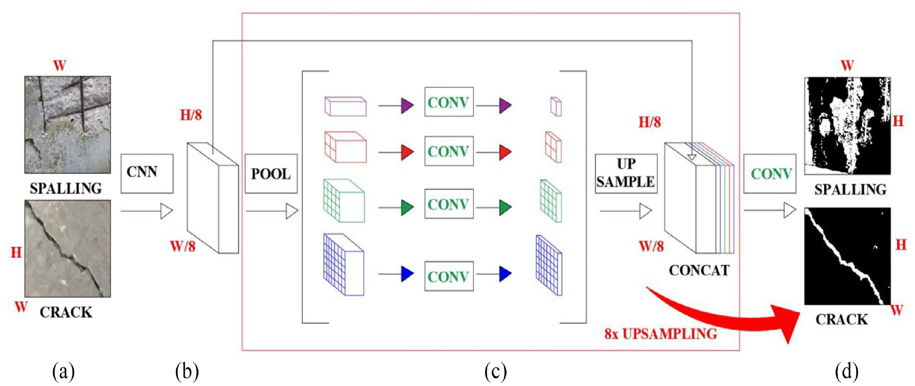
Schematic diagram of PSP-Net (a) Input layer, (b) feature map, (c) pyramid pooling module, and (d) final predictions.

Details of defects classification

Training configuration and evaluation metrics

For this study, three types of CNN-classifiers are used—(a) VGG19, (b) ResNet50 and (c) InceptionV3. To train the CNN models, the pretrained weights of ImageNet (1.2 million images with 1000 categories) are examined to achieve the efficiency of classifying the type of the defect—crack and spalling.

As Goodfellow et al. ⁵¹ stated, the epoch size, batch size, and optimization function are the most important parameters for an optimized convergence. For classification models, these parameters’ values are selected after carefully analyzing the learning process with a variety of hyper-parameter values to achieve the best output. Finally, the networks are trained for 100 epochs for image classification, and the models are evaluated based on their performance. An epoch refers to the entire neural network training process in one cycle, including a forward pass and a backward pass. Forward Pass indicates the calculation process from the first layer to the last layer, and backpropagation refers to updating the weights by reducing learning loss. Two functions, that is, the early-stopping function and the reduced learning rate, are introduced for the training purpose. This function helps the model avoid overfitting in the learning process and reduces the computational cost. After analyzing all the combinations, it is observed that all the models reached their convergence point within 100 epochs. A batch size of 10 is used to feed the images in the network, and ReLu (Rectified Linear Unit) activation function is introduced to help the model learn complex patterns. For optimization, the networks have used SGD and RMSprop. According to some previous studies, SGD and RMSprop are frequently utilized optimizers for CNN model training.^52–54 The size of the epoch, batch size, and the optimization function were selected after carefully analyzing the learning process to achieve the best output. Regarding the optimization algorithm, a loss function helps the model guide through the right learning direction while minimizing the prediction error. For this study, cross-entropy (CE) loss function is used and the formulation is shown in Equation (3).

$${\mathrm{Loss}}_{\mathrm{CE}}=-(x\log \left(x^{\prime }\right)+\left(1-x\right)\log (1-x^{\prime }))$$

(3)

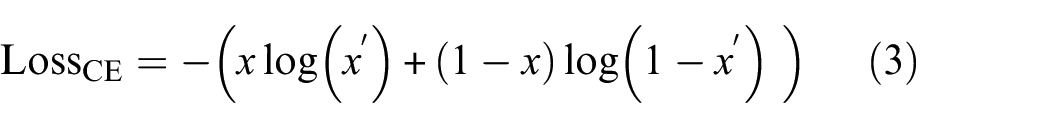
Here, $x$ and $x^{\prime }$ denotes the ground truth and prediction. The value of $x$ is equal to “0 (crack)” or “1 (spalling)” and the prediction of $x^{\prime }$ can be either “0” or “1.”

Four evaluation metrics, accuracy (Equation (4)), precision (Equation (5)), recall (Equation (6)), and confusion matrix, are used to evaluate the performance of the aforementioned models. The following are formulations for the evaluation metrics:

$$\mathrm{Accuracy}=\frac{\mathrm{TP}+\mathrm{TN}}{\mathrm{TP}+\mathrm{TN}+\mathrm{FP}+\mathrm{FN}}$$

(4)

$$\mathrm{Precision}=\frac{\mathrm{TP}}{\mathrm{TP}+\mathrm{FP}}$$

(5)

$$\mathrm{Recall}=\frac{\mathrm{TP}}{\mathrm{TP}+\mathrm{FN}}$$

(6)

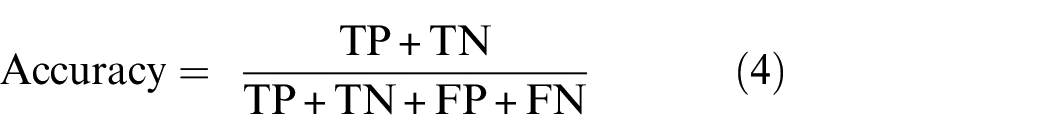
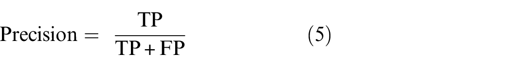
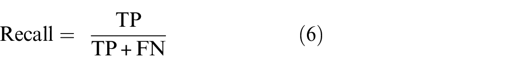
TP = True Positive, TN = True Negative, FP = False Positive, FN = False Negative

Here, TP denotes if the crack image is classified correctly while TN shows if the spalling image is classified correctly. Whereas, FP means if the crack image is classified incorrectly while FN represents if the spalling image is classified incorrectly. The confusion matrix shows a summarized graphical presentation of TP, TN, FP, FN.

The networks are developed using Keras ⁵⁵ applications, written in Python, backend by TensorFlow and analyzed using Google Collaboratory.

Results for defects classification

This study has focused on different optimization functions and learning rates for sensitivity analysis. Table 4 shows that among the three models, the InceptionV3 model has got the best accuracy, followed by ResNet50 and VGG19. One of the possible reasons for InceptionV3 to outperform others is that it focuses on reducing computational costs while going deeper to achieve an optimized performance. Meanwhile, ResNet tries to achieve the convergence point without concerning the optimization, which introduces overfitting issues in the training process, which finally affects the model’s prediction accuracy.

Table 4.

Summary results of defects classification models.

CNN models	Learning rate	Accuracy		Precision		Recall
		SGD (%)	RMSprop (%)	SGD (%)	RMSprop (%)	SGD (%)	RMSprop (%)
*InceptionV3	0.1	86	88	78	82	100	97
	0.001	91	89	83	79	100	100
	0.0001	84	89	81	84	94	100
ResNet50	0.1	85	87	72	76	97	100
	0.001	82	87	69	77	89	97
	0.0001	79	85	69	74	89	97
VGG19	0.1	63	65	60	62	81	82
	0.001	61	62	64	68	80	84
	0.0001	63	67	61	62	82	86

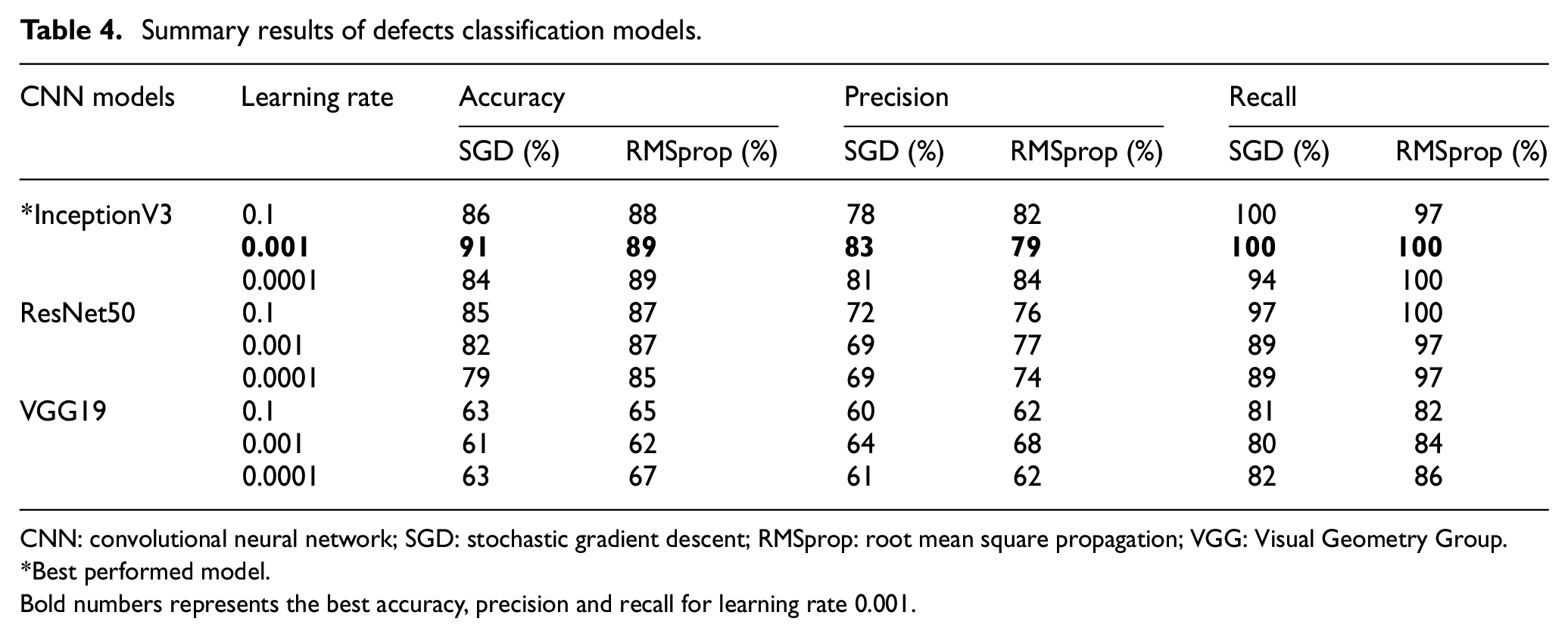
CNN: convolutional neural network; SGD: stochastic gradient descent; RMSprop: root mean square propagation; VGG: Visual Geometry Group.

*

Best performed model.

Bold numbers represents the best accuracy, precision and recall for learning rate 0.001.

The defect classification models are analyzed using the SGD and RMSprop optimization function and three different depths of learning rate—0.1, 0.001, and 0.0001, where the learning rate of 0.001 showed the best performance (Table 4). While training with a learning rate of 0.1, the model skipped many features, which has ultimately reduced the model’s prediction accuracy, whereas, with a learning rate of 0.0001, the training process has taken a slow pace raising the computation cost without actually increasing the accuracy. From Figure 9 it is prominent that with optimizer SGD, InceptionV3 has the best performance with an accuracy of 91%, precision of 82%, and recall of 100%. In a previous study, it was stated that while training the CNN models, SGD has the better generalization capacity and stability rather than the adaptive optimization functions (i.e., RMSprop), which eventually helps the model to reach its optimization point better than others. ⁵⁶ Also, Wilson et al. ⁵⁷ studied experimental and empirical analysis for CNN classification models, concluding that SGD has better converged proficiency than adaptive optimizers.

Figure 9.

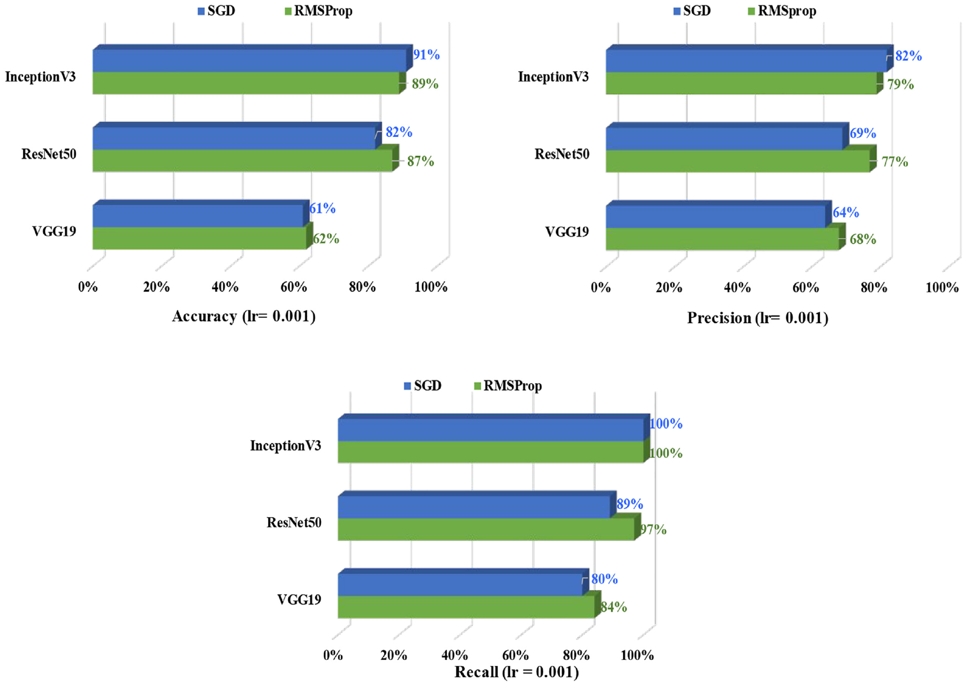
Defects classification: comparison of the evaluation metrics based on SGD and RMSprop optimization function for learning rate 0.001.

Another evaluation metric, the confusion matrix in Figure 10 gives a closer look at the true and predicted labels distribution for crack and spalling. For the confusion matrix diagram, the x-axis and y-axis represent the true label and predicted label, respectively, where “0” denotes the crack and “1” refers to “spalling.” Among the 57 crack test images, the InceptionV3 model identified 49 images successfully, whereas the model successfully identified all 39 spalling test images. For the classification of crack and spalling test dataset, InceptionV3 has correctly identified the crack and spalling images with 86 and 100% accuracy, respectively.

Figure 10.

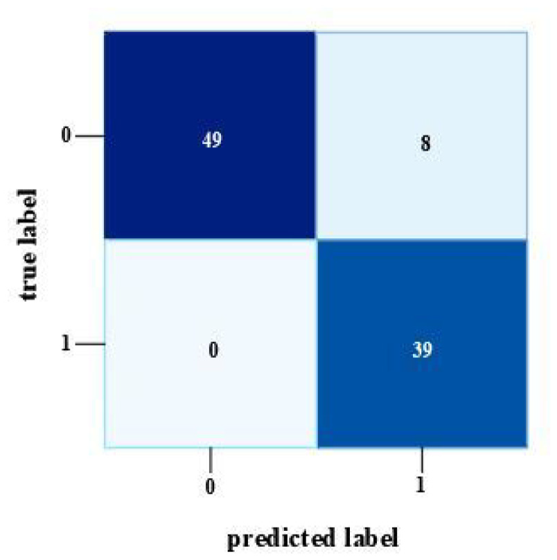
Confusion matrix for InceptionV3.

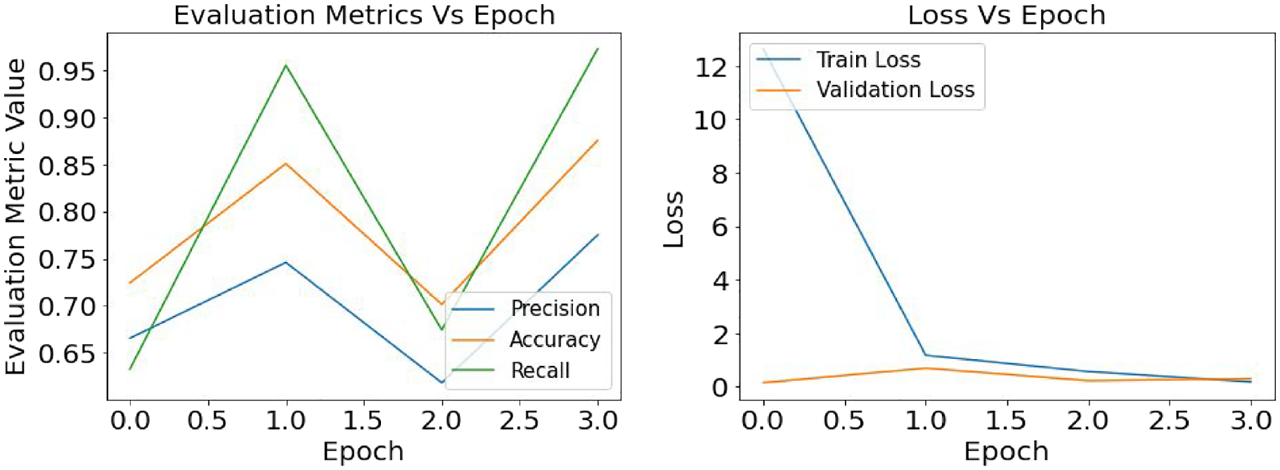
As mentioned earlier in this study loss function helps the model to understand the difference between the true value and predicted value and directs the model to reduce the losses while training the weights. Figures 11, 12, and 13 present the graphical understanding of the loss distribution of the InceptionV3 model for three learning rates 0.1, 0.001, and 0.0001. From all the graphs, it is prominent that in the training module with a learning rate of 0.001, the InceptionV3 model has the least loss while the model has achieved an accuracy, precision, and recall close to 100%.

Figure 11.

Defects classification with InceptionV3: result of the evaluation metrics and model loss for optimizer SGD and learning rate 0.0001.

Figure 12.

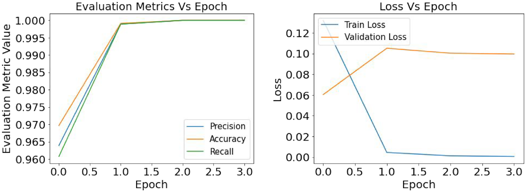
Defects classification with InceptionV3: result of the evaluation metrics and model loss for optimizer SGD and learning rate 0.001.

Figure 13.

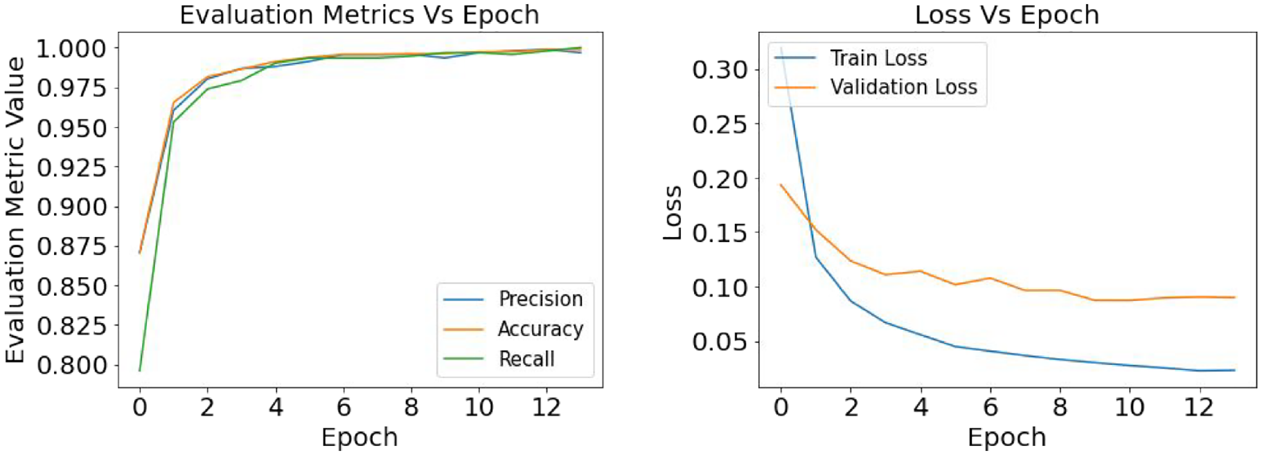
Defects classification with InceptionV3: result of the evaluation metrics and model loss for optimizer SGD and learning rate 0.1.

After comparing all the models, it can be observed that InceptionV3’s deepest and most complex learning layers have helped the model to achieve robust performance. A few sample results of defects identification are presented in Figure 14(a) and (b), where the first sentence describes the prediction result, and the second line shows the type of the actual defect. Figure 14(a) clearly indicates that for InceptionV3, most of the cracks are predicted with 100% accuracy, and the rest have more than 90% accuracy. Also, the VGG19 model has the least crack prediction accuracy, even with some false predictions. Figure 14(b) shows that similar to crack prediction, the InceptionV3 model also performed best for spalling detection and VGG19 has the least accuracy.

Figure 14.

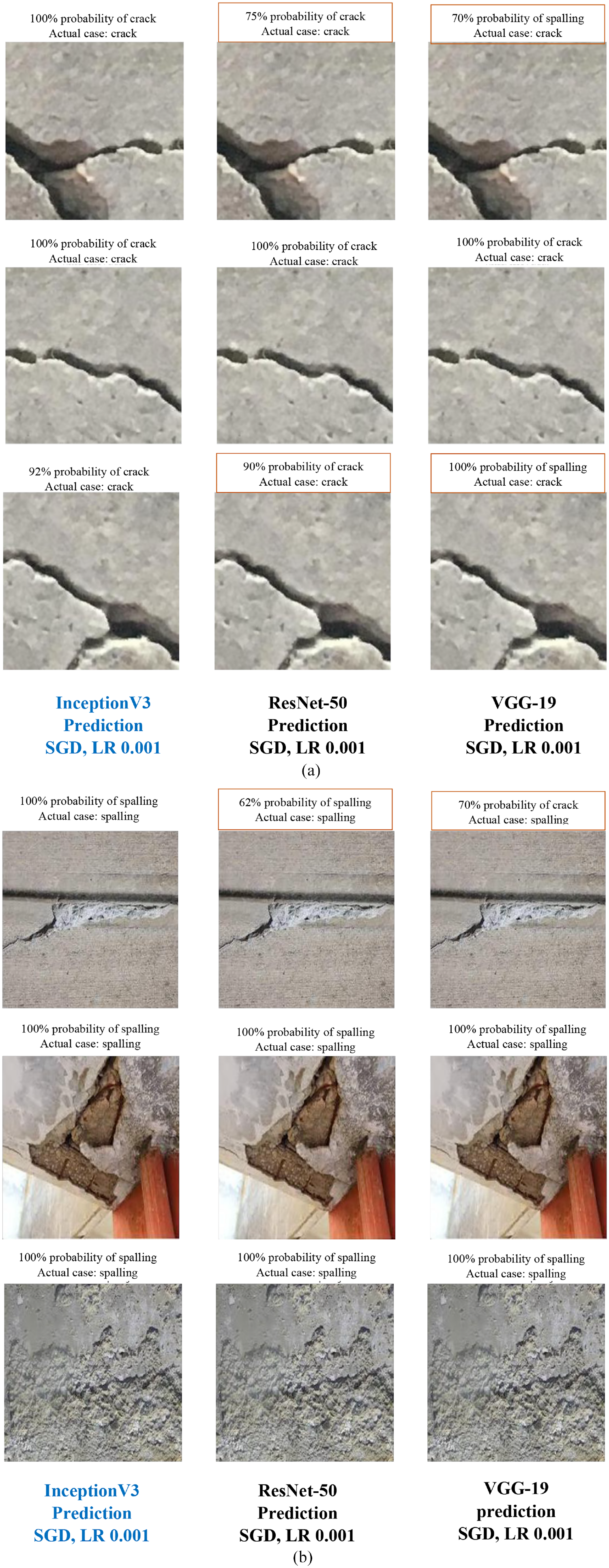
Sample images for defects identification using InceptionV3 model. (a) Crack prediction and (b) spalling prediction.

Semantic segmentation of defects

Training configuration and evaluation metrics

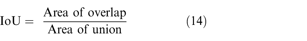
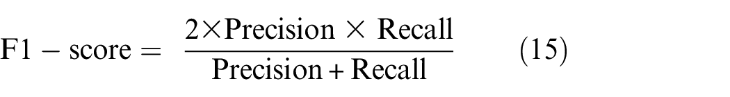
The encoder-decoder model with U-Net and PSP-Net architectures is used for the semantic segmentation process. The encoder part of both U-Net and PSP-Net architecture is built with four different backbone models—VGG19, ResNet50, InceptionV3, and EfficientNetB3. As mentioned earlier, sensitivity analysis is performed for the semantic segmentation, and the hyper-parameters are nominated based on model’s optimized output. Each network has gone through 100 epochs to train the models, and a batch size of five images is applied. Similar to the classification technique, two optimizers—SGD and ADAM are designated for defects segmentation. Also, three different depth of learning rates 0.1, 0.01, and 0.0001 are considered in both crack and spalling segmentation cases and ReLu is used as an activation function. To initialize the weight training, ImageNet weights are used for segmentation, and later the specific weights considered for this study are implemented for case-specific performance evaluation. In the context of the loss function, a summation of dice loss and focal loss is applied. Focal loss is an improved version of CE loss used to solve the class imbalance problem between easy and hard examples, where misclassified examples are penalized with higher weights. On the other hand, Dice loss only considers the imbalance between the foreground and background of the images, overlooking the imbalance between easy and hard samples. Combining these two loss functions, Focal Dice Loss proposes a novel balanced sampling system that helps the network focus on hard examples more than the easy ones. ⁵⁸ For semantic segmentation, generally, IoU and F1-score are considered. Apart from these two, precision and recall metrics are also applied here. IoU quantifies the overlap area between the original and predicted image, and the F1-score is a harmonic mean of the combination of precision and recall metrics. Therefore, F1-score is one of the most indicative metrics to identify the best-performed network. Equations (14) and (15) presents the formulation of IoU and F1-score.

$$\mathrm{IoU}=\frac{\mathrm{Area}\mathrm{of}\mathrm{overlap}}{\mathrm{Area}\mathrm{of}\mathrm{union}}$$

(14)

$$\mathrm{F}1-\mathrm{score}=\frac{2\times \mathrm{Precision}\times \mathrm{Recall}}{\mathrm{Precision}+\mathrm{Recall}}$$

(15)

Results for crack semantic segmentation

Crack semantic segmentation: U-Net model

This section presents the crack detection results using U-Net semantic segmentation based on four CNN backbone models. A training dataset of 2861 images and a validation dataset of 817 images are used to validate the training performance of all four models. During the testing phase, all four models used their own pretrained model’s weights to predict the crack areas on the test images (409 images). The summary of all the 24 models’ results for crack segmentation is presented in Table 5. Among all the models, EfficientNetB3-based U-Net has achieved a maximum IoU score of 91.98%, an F1-score of 95.66%, a precision score of 94.73%, and recall score of 97.59%. Also, the ADAM optimizer and learning rate of 0.01 has facilitated the model to obtain the optimized performance.

Table 5.

Evaluation summary of U-Net-based crack segmentation models’ results depending on different optimizers and learning rate.

Evaluation metrics	Learning rate	U-Net		U-Net		U-Net		U-Net
		EfficientNetB3		InceptionV3		ResNet50		VGG19
		SGD	ADAM	SGD	ADAM	SGD	ADAM	SGD	ADAM
IoU	0.1	87.81	80.64	86.61	86.59	89.50	87.61	86.81	80.64
	*0.01	89.40	*91.98	88.81	91.83	91.91	89.55	87.35	89.54
	0.0001	88.67	90.05	88.83	91.46	90.85	82.02	83.59	91.27
F1-score	0.1	92.75	88.17	92.29	92.19	94.11	92.89	92.35	88.17
	*0.01	94.09	*95.66	93.66	95.53	95.62	94.16	92.76	94.14
	0.0001	93.66	94.47	93.62	95.32	94.58	89.42	90.42	95.21
Precision	0.1	93.38	80.64	91.97	95.31	92.86	92.99	89.95	80.64
	*0.01	93.90	*94.73	95.04	93.82	93.42	94.54	95.81	95.00
	0.0001	92.84	93.86	94.16	94.42	94.58	85.73	92.65	93.97
Recall	0.1	93.72	100	93.14	90.16	95.54	93.45	95.28	100
	*0.01	94.57	*97.59	92.74	97.35	97.97	93.94	90.41	93.47
	0.0001	94.42	94.38	93.54	96.25	95.36	94.94	88.55	96.52

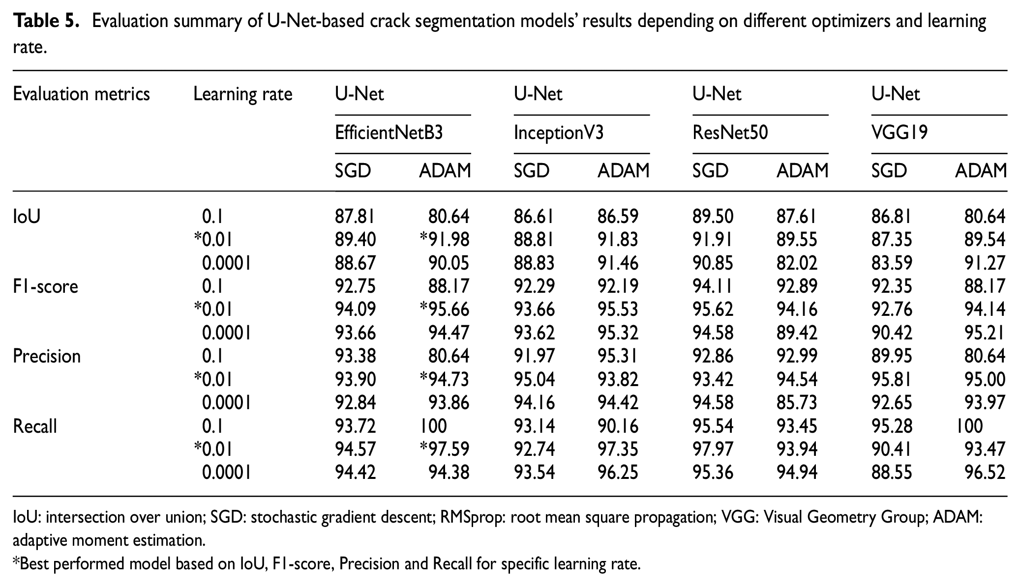
IoU: intersection over union; SGD: stochastic gradient descent; RMSprop: root mean square propagation; VGG: Visual Geometry Group; ADAM: adaptive moment estimation.

*

Best performed model based on IoU, F1-score, Precision and Recall for specific learning rate.

In Figure 15, the crack semantic segmentation performance of U-Net is compared with optimizers SGD and ADAM. Figure 15 represents that for crack detection, all networks have achieved the best performance using the optimization function ADAM indicating that with ADAM, the model has recognized the most crack features with a limited computational cost. This statement agrees with the findings of some previous studies that ADAM is the best optimizer.^39,42 After studying the state-of-the-art performance of nine different optimizers on the segmentation process, Yaqub et al. ⁴² found that ADAM is the best optimizer. Choi and Cha ²⁷ claimed that with the best tuned model, adaptive optimizers have better generalization potential than gradient-based optimizers. Also, ADAM has distinctive features like the momentum and adaptive learning method, which helps the model converge faster than any other optimizer.

Figure 15.

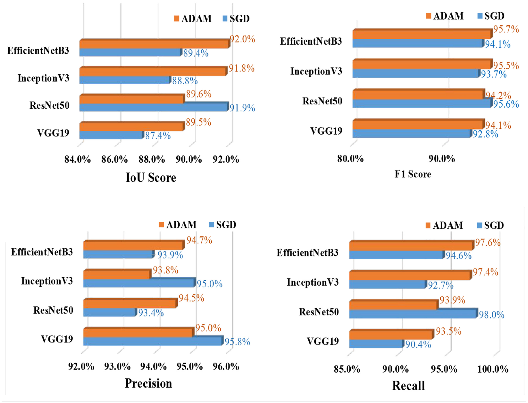
Crack segmentation: U-Net—comparison of the evaluation metrics based on SGD and ADAM optimizers for learning rate 0.01.

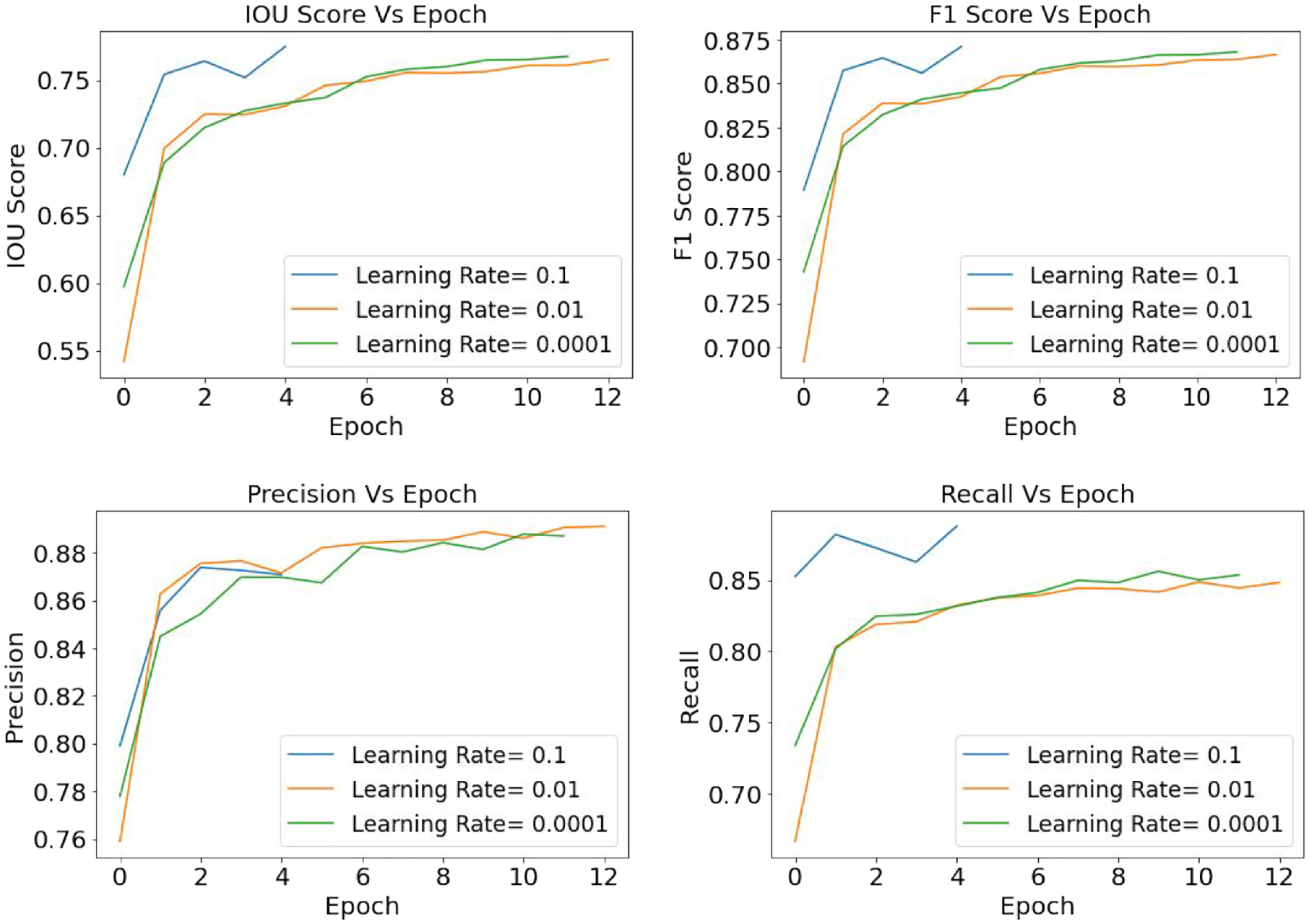
Figure 16 illustrates the different evaluation metric values for three different learning rates 0.1, 0.01, and 0.0001, for EfficientNetB3-based U-Net model. From Figure 16 it is clearly visible that with a learning rate of 0.01, the model has the most training performance with 40 epochs, indicating that with a learning rate of 0.01, the model has learnt the defect features more precisely than other learning rates. Also, similar to defects classification, the learning rate of 0.01 has the optimal performance, while the learning rate of 0.1 has skipped many features from the image, and the learning rate of 0.0001 has only slowed down the model’s training without contributing to prediction accuracy.

Figure 16.

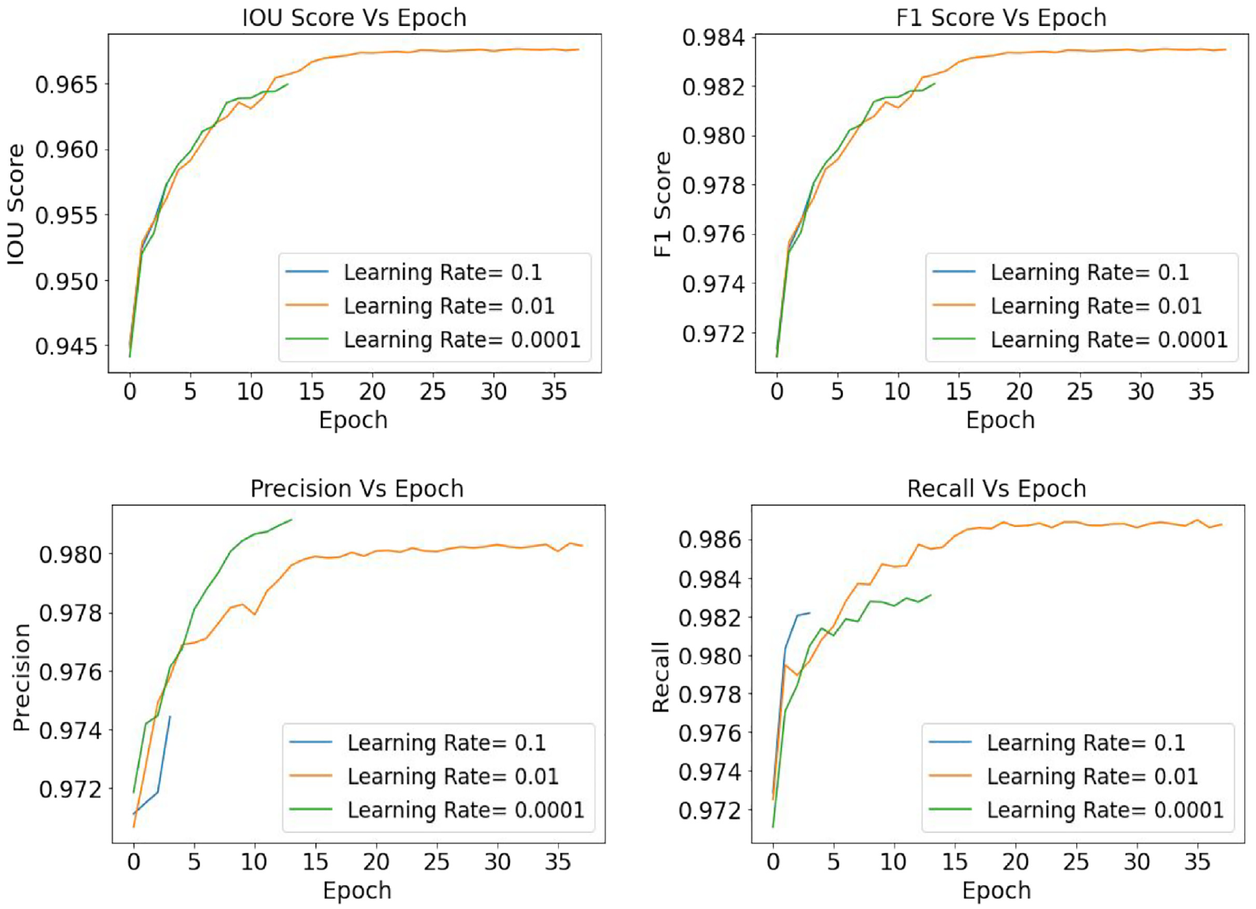
Crack segmentation: U-Net (EfficientNetB3)—comparison of the evaluation metrics based on ADAM optimizers and learning rate 0.1, 0.01, and 0.0001.

Among all the models, EfficientNetB3 achieved a maximum F1-score of 92.1%, IoU 84.6%, precision 90.9%, and recall 91.8%. Figure 15 illustrates some sample crack detection images performed by EfficientNetB3 where ground truth images are created using the threshold method, and prediction images are the final output of the trained model. For crack detection, EfficientNetB3 attained the best performance. One of the possible reasons behind this is that the EfficientNet model’s architecture is developed based on an optimized depth, width, and high-resolution learning process. This optimized condition has helped the model to identify and learn the complex features of the images in a high pixel-depth without losing much information.

Crack semantic segmentation: PSP-Net model

Table 6 summarizes the outputs of 24 models for crack segmentation utilizing PSP-Net, and it is highlighted that most of the best performance is achieved with a learning rate of 0.01 and optimizer ADAM. Table 6 shows that among all the models, EfficientNetB3-based PSP-Net has outranked all the other models and achieved a maximum IoU value of 89.55%, F1-score 94.13%, precision value of 92.56%, and recall value of 95.94%. Figure 17 presents the models’ performance values for two different optimizers, that is, SGD and ADAM, with a learning rate of 0.01.

Table 6.

Evaluation summary of PSP-Net-based crack segmentation models’ results depending on different optimizers and learning rate.

Evaluation metrics	Learning rate	PSP-Net		PSP-Net		PSP-Net		PSP-Net
		EfficientNetB3		InceptionV3		ResNet50		VGG19
		SGD	ADAM	SGD	ADAM	SGD	ADAM	SGD	ADAM
IoU	0.1	81.56	85.39	81.59	84.43	74.56	80.82	72.39	78.49
	*0.01	86.03	*89.55	84.33	87.64	76	83.2	74.4	80.7
	0.0001	85.65	88.59	83.41	86.75	77.01	82.96	73.69	79.58
F1-score	0.1	89.95	91.22	88.76	91.38	83.74	83.85	83.94	83.12
	*0.01	91.30	*94.13	90.98	92.83	85.6	86	85.3	88.1
	0.0001	90.89	93.97	89.35	91.45	84.59	85.38	84.58	87.65
Precision	0.1	91.88	90.10	85.38	90.33	79.58	85.49	81.24	89.58
	*0.01	93.07	*92.56	89.67	91.74	82.2	88.6	83.4	92.2
	0.0001	92.03	92.45	88.96	91.57	82.59	87.96	82.87	91.97
Recall	0.1	90.39	91.74	91.24	90.84	82.38	88.23	81.64	85.38
	*0.01	92.31	*95.94	93.10	91.62	85.3	90.4	84.7	88.4
	0.0001	91.76	94.39	92.40	90.88	84.79	89.54	83.67	87.57

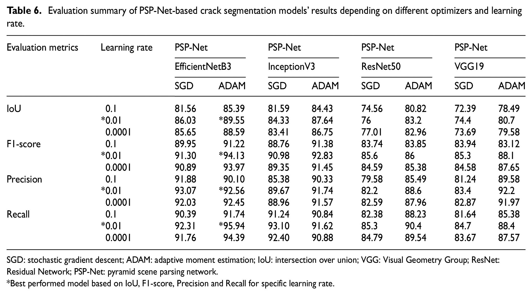
SGD: stochastic gradient descent; ADAM: adaptive moment estimation; IoU: intersection over union; VGG: Visual Geometry Group; ResNet: Residual Network; PSP-Net: pyramid scene parsing network.

*

Best performed model based on IoU, F1-score, Precision and Recall for specific learning rate.

Figure 17.

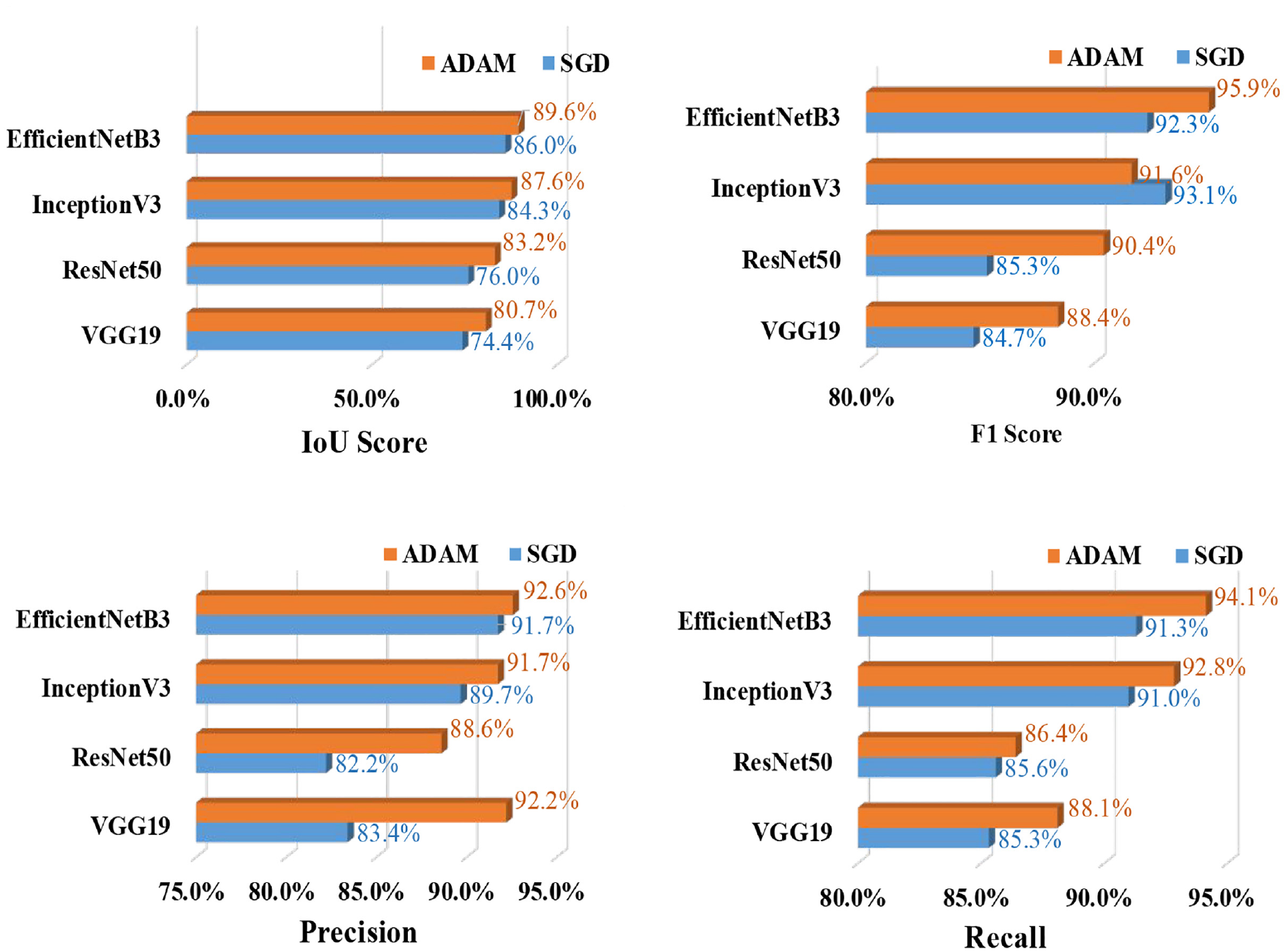
Crack segmentation: PSP-Net—comparison of the evaluation metrics based on SGD and ADAM optimizers and learning rate 0.01.

Figure 18 illustrates that with a learning rate of 0.01, EfficientNetB3-based PSP-Net has trained for 40 epochs, which is also the maximum epoch size of other learning rates of 0.1 and 0.0001. Also, during the training process, the abovementioned model has gained performance higher than 95% for all the evaluation metrics, that is, IoU, F1-score, precision, and recall.

Figure 18.

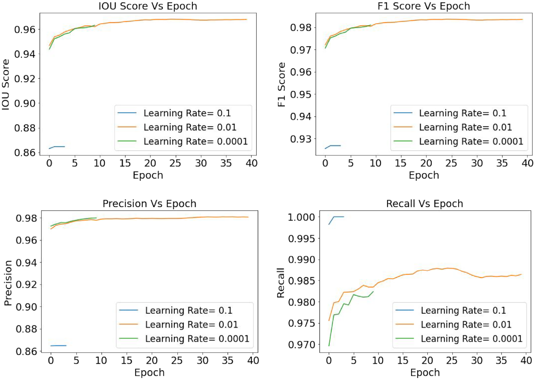
Crack segmentation: PSP-Net (EfficientNetB3)—comparison of the evaluation metrics based on ADAM optimizers and learning rate 0.1, 0.01, and 0.0001.

After analyzing both the U-Net and PSP-Net models for crack semantic segmentation, it is evident that EfficientNetB3-based U-Net has the best performance, while optimizer ADAM has shown superiority over other hyper-parameter values. Also, the learning rate of 0.01 has exhibited efficient weight learning steps to achieve optimal performance. After comparing Tables 5 and 6, it is observed that the EfficinetNetB3-based both U-Net and PSP-Net models have a quite similar performance which eventually agrees on the proficiency of encoder-decoder models for semantic segmentation of objects.

Results for spalling semantic segmentation

Spalling semantic segmentation: U-Net model

Training and a validation dataset of 770 and 220 images are considered for spalling segmentation, respectively. Following a similar sensitivity analysis approach as crack segmentation, the spalling semantic segmentation has also considered SGD and ADAM optimizers. Table 7 presents the performance of the U-Net models for spalling segmentation based on four backbone models, three learning rates, and two optimizers. From Table 7 and Figure 19 it is found that for spalling segmentation, ADAM performed better than SGD, and InceptionB3 outperformed the rest of the models. This InceptionV3-based U-Net model has achieved the best training performance with an IoU value of 81.30%, F1-score of 89.43%, the precision value of 86.40%, and recall value of 92.87%.

Table 7.

Evaluation summary of U-Net-based spalling segmentation models’ results depending on different optimizers and learning rate.

Evaluation metrics	Learning rate	U-Net		U-Net		U-Net		U-Net
		EfficientNetB3		InceptionV3		ResNet50		VGG19
		SGD	ADAM	SGD	ADAM	SGD	ADAM	SGD	ADAM
IoU	0.1	72.33	50.30	72.03	74.69	63.66	70.63	65.38	56.10
	*0.01	77.16	78.10	77.31	*81.30	80.78	74.68	74.98	81.28
	0.0001	40.01	79.53	36.37	79.90	81.86	42.19	72.32	81.46
F1-score	0.1	83.16	49.05	83.03	84.88	76.37	81.93	78.24	69.55
	*0.01	86.73	87.30	86.75	*89.43	89.13	84.95	85.10	89.42
	0.0001	55.39	88.30	52.35	88.52	89.79	58.22	83.24	89.56
Precision	0.1	88.28	77	85.33	87.45	95.66	88.49	79.21	56.20
	*0.01	87.70	88.58	87.20	*86.40	82.02	84.86	85.94	88.38
	0.0001	59.65	85.65	56.86	86.07	86.64	58.43	88.32	83.73
Recall	0.1	79.66	51.24	82.20	82.87	65.53	77.48	78.03	66.34
	*0.01	85.93	86.27	86.57	*92.87	97.92	83.34	82.61	93.31
	0.0001	56.00	91.24	51.86	91.29	93.22	62.08	79.37	96.48

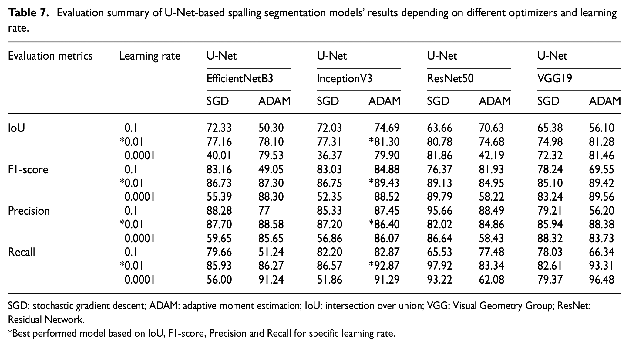
SGD: stochastic gradient descent; ADAM: adaptive moment estimation; IoU: intersection over union; VGG: Visual Geometry Group; ResNet: Residual Network.

*

Best performed model based on IoU, F1-score, Precision and Recall for specific learning rate.

Figure 19.

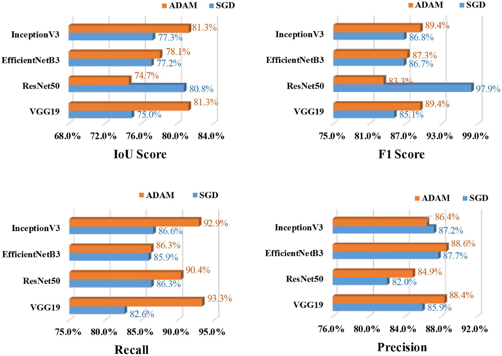
Spalling segmentation: U-Net (InceptionV3)—comparison of the evaluation metrics based on SGD and ADAM optimizers and learning rate 0.01.

Subsequently, the best-performed model, InceptionV3, is analyzed for learning rates of 0.1, 0.01, and 0.0001 and results are summarized in Figure 20. From the graphs, it is prominent that the model training has kept a straight line over the epochs indicating that during the training process, the model attained its convergence quite early. The probable explanation for this scenario is that to build the ground truth mask, this study has applied a generalized annotation system which could have affected the learning process.

Figure 20.

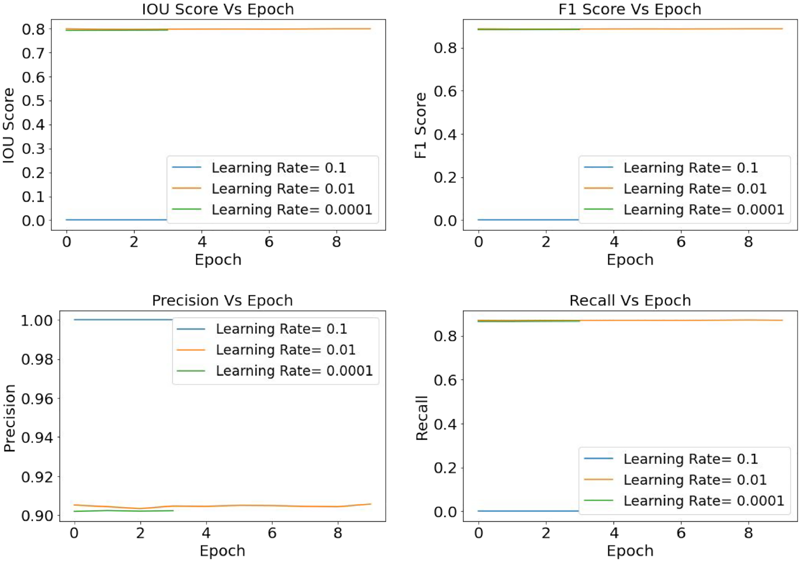
Spalling segmentation: U-Net (InceptionV3)—comparison of the evaluation metrics based on ADAM optimizers and learning rate 0.1, 0.01, and 0.0001.

Spalling semantic segmentation: PSP-Net model

Similar to U-Net analysis PSP-Net model is also analyzed for four CNN backbone models, and the results are summarized in Table 8 and Figure 21. From Table 8, it is found that the PSP-Net has obtained the best performance with the backbone CNN model EfficientNetB3 and similar to previous segmentation model optimizer ADAM and learning rate 0.01 has showed the most efficient performance. Also, Figure 22 illustrates the performance of EfficientNetB3-based PSP-Net for three different learning rates 0.1, 0.01, and 0.0001. In this case, with a learning rate of 0.01, the model has the maximum learning epochs and the best numerical value of evaluation metrics. These abovementioned values indicate that ADAM is the best optimizer and a learning rate of 0.01 is the most effective learning step to train the model.

Table 8.

Evaluation summary of PSP-Net-based spalling segmentation models’ results depending on different optimizers and learning rate.

Evaluation metrics	Learning rate	PSP-Net		PSP-Net		PSP-Net		PSP-Net
		EfficientNetB3		InceptionV3		ResNet50		VGG19
		SGD	ADAM	SGD	ADAM	SGD	ADAM	SGD	ADAM
IoU	0.1	68.34	69.68	62.59	61.24	59.32	71.84	58.48	64.38
	*0.01	70.78	*75.30	66.89	65.09	60.66	74.67	63.94	68.76
	0.0001	70.43	74.31	63.91	64.91	61.24	73.72	61.38	65.10
F1-score	0.1	79.75	79.47	71.34	73.80	69.47	80.46	72.40	76.61
	*0.01	82.25	*85.28	79.10	77.51	73.60	84.84	77.13	80.63
	0.0001	81.86	84.83	74.49	76.42	71.56	82.35	76.39	80.54
Precision	0.1	81.05	80.25	76.29	75.39	72.38	85.66	77.05	85.98
	*0.01	84.10	*86.88	81.64	77.43	78.25	88.45	79.28	86.9
	0.0001	85.63	85.44	79.50	78.23	76.77	87.30	78.98	87.20
Recall	0.1	80.88	81.40	70.94	77.86	69.58	79.66	73.44	74.23
	*0.01	82.08	*84.41	78.90	81.87	72.97	82.31	75.89	76.28
	0.0001	81.37	84.34	77.48	81.36	72.45	81.98	74.09	75.20

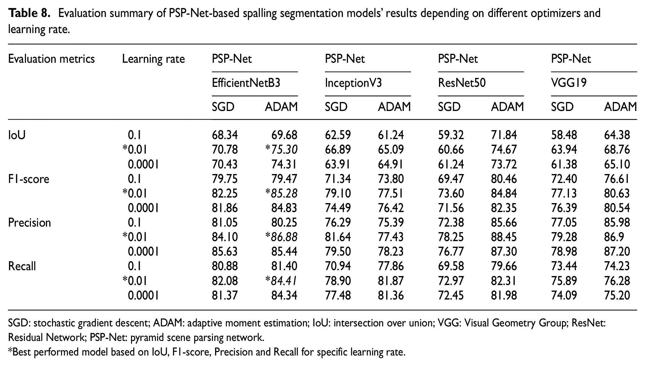
SGD: stochastic gradient descent; ADAM: adaptive moment estimation; IoU: intersection over union; VGG: Visual Geometry Group; ResNet: Residual Network; PSP-Net: pyramid scene parsing network.

*

Best performed model based on IoU, F1-score, Precision and Recall for specific learning rate.

Figure 21.

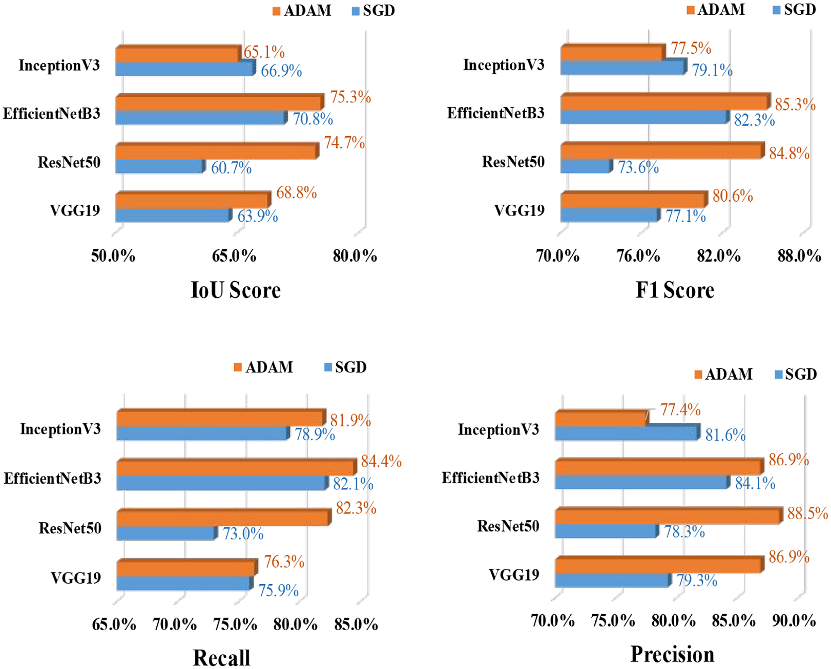
Spalling segmentation: PSP-Net (EfficientNetB3)—comparison of the evaluation metrics based on SGD and ADAM optimizers and learning rate 0.01.

Figure 22.

Spalling segmentation: PSP-Net (EfficientNetB3)—comparison of the evaluation metrics based on ADAM optimizers and learning rate 0.1, 0.01, and 0.0001.

After analyzing both U-Net and PSP-Net models for spalling segmentation, it can be witnessed that InceptionV3-based U-Net has outranked all the other models, followed by EfficientNetB3-based PSP-Net. Some of the sample images of concrete crack and spalling segmentation prediction by the best-performed models are presented in Figures 23 and 24, respectively. Here in the image section, the column indicates the original images of defects, and the second column shows the ground truth mask dataset. The rest of the two columns indicate the prediction done by the U-Net model and PSP-Net model, respectively. The graphs show that the crack area prediction quality is relatively similar for both models, with a slightly better performance with U-Net.

Figure 23.

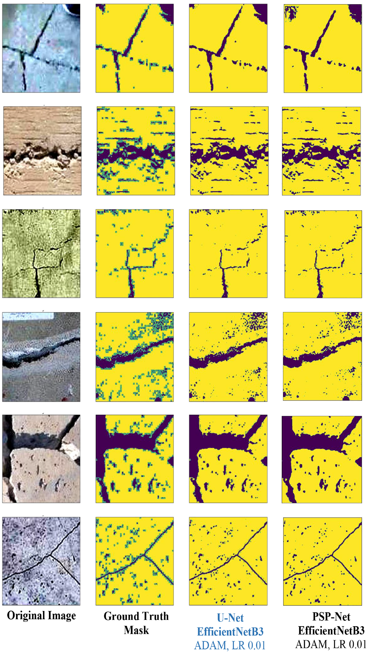
Semantic segmentation of crack detection using best two models.

Figure 24.

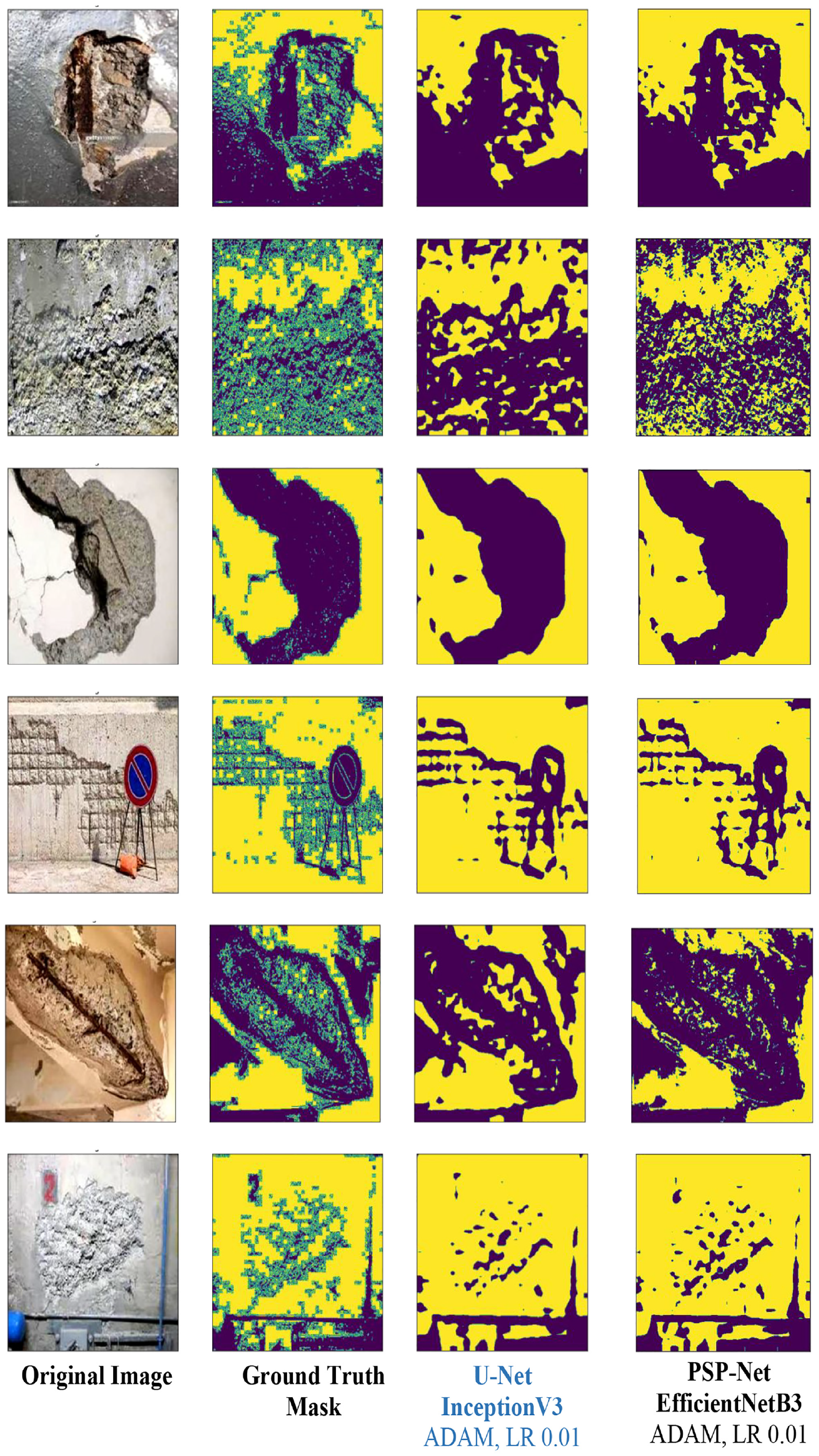
Semantic segmentation of spalling detection using best two models.

Conclusion

This study developed a DL-based automated concrete defects identification and classification model using CNN algorithms. Three different types of pre-built CNN models—VGG19, ResNet50, and InceptionV3 are used to compare the performance of defects categorization models. For semantic segmentation, two encoder-decoder models are proposed—U-Net and PSP-Net architecture and used four backbone models, namely—VGG19, ResNet50, InceptionV3, and EfficentNetB3, to evaluate the performance of the best defect detection model. A crack dataset of 4087 images and a spalling dataset of 1100 images are used for classification and segmentation techniques. The RGB images are processed into 224 × 224 pixel resolution and divided into training, validation, and testing datasets with a split of 70:20:10. Based on the performance of CNN algorithms, the following conclusions are drawn from this study:

• As the performance of CNN models is highly dependent on a diverse dataset, this study has developed a concrete defects image dataset (4087 crack images and 1100 spalling images) with background noises to replicate the realistic inspection scenario. The images are collected from real-time inspection reports of local industry partner and web-based resources. The developed dataset is the largest to date for both crack and spalling with real-time inspection images and without any image augmentation process implication.

• For sensitivity analysis of CNN-classifiers, this study used two different optimization functions, that is, SGD and RMSprop and three learning rates 0.1, 0.001, and 0.0001. Comparing the three learning rates’ performance, the finest performance is achieved by using a learning rate of 0.0001. InceptionV3 with optimizer SGD and learning rate 0.001 performed best, which indicates that in CNN training, a lower learning rate does not give surety for better performance and sometimes it can increase the model’s computational cost without significantly improving the performance.

• Using the pretrained weights from ImageNet, the CNN-classifier InceptionV3 successfully identified defects (i.e., crack and spalling) and presented the best prediction results with the test dataset. The model has an overall accuracy of 91%, precision of 83%, and recall of 100%. Also, the confusion matrix indicated that the model has successfully identified spalling images with 100% accuracy, whereas the crack identification accuracy is 86%.

• For CNN segmentation of defects, SGD and ADAM optimization functions are used. In crack detection, SGD has performed better than ADAM, whereas, in spalling segmentation, ADAM has shown the best performance. Crack and spalling segmentation gained the best output in the training phase by using a learning rate of 0.01.

• Two encoder-decoder models with U-Net and PSP-Net architecture are proposed for the semantic segmentation of defects. The encoder model is mainly responsible for feature extraction from the image and is built on four types of backbone models. On the other hand, the decoder part is used for up-sampling the image features to build a sparse feature map. After completing the training, for crack segmentation, EfficientNetB3-based U-Net architecture outperformed the other models, whereas InceptionV3-based U-Net performed much better than other models for spalling segmentation.

• For crack area detection, the EfficientNetB3-based U-Net model gained F1-score of 95.66%, IoU of 91.98%, precision of 94.73%, and recall of 97.59%. In case of spalling area detection, the recorded testing evaluation metrics values are found to be F1-score 89.43%, IoU 81.30%, precision 86.40%, and recall 92.87% for InceptionV3-based U-Net model.

• Even though U-Net performs better in the crack and spalling segmentation, it is also evident that PSP-Net models also obtained a performance adjacent to U-Net models, where all the evaluation values are higher than 80%, which certainly glorifies the overall architecture of encoder-decoder models.

Even with the satisfactory performance of the proposed models, future studies are substantially encouraged to obtain a more precise prediction. One of the biggest challenges this study has encountered is the crack and spalling dataset size imbalance. The crack dataset consists of 4087 images, whereas the spalling dataset has 1100 images (almost one-fourth of crack dataset). Also, collecting images with complex background replicating the original site condition is relatively difficult. Some previous research collected concrete crack images for crack identification but in case of other types of defects (i.e., concrete spalling) open-source dataset is not easily available. To build a comprehensive concrete defects detection model, future research should develop defects dataset from original site inspection reports. Future studies should also focus on analyzing all possible types of defects in concrete structures.