
Abstract
Information on the presence and location of cracks in civil structures can be precious to support operators in making decisions related to structural management and scheduling informed maintenance. This paper investigates the efficacy of supervised machine learning to solve the inverse electrical impedance tomography problem and to reconstruct the conductivity distribution of a piezoresistive sensing film. This film consists of a conductive paint applied onto structural components, and operators can use its conductivity distribution to identify crack sizes and locations in the underlying structure. A deep neural network is employed to reconstruct a dense conductivity distribution within the painted area by using only voltage measurements collected at sparse boundary locations. Since one of the most challenging aspects of using supervised learning tools for real-world applications is generating a representative training dataset, this paper presents a new approach to test the suitability of synthetic datasets built using a finite element model of the sensing film. Results are reported for four sensing specimens fabricated with two different techniques (i.e., using carbon nanotubes and graphene nanosheets, respectively). Crack-like damage is induced to the substrate of the sensing film and identified using the proposed machine learning technique. Promising results are obtained as compared to conventional methods.
Keywords
Introduction
Several structural health monitoring (SHM) strategies have been proposed in the last few decades for the early detection of structural anomalies resulting from repeated load cycles, material degradation or strong and exceptional events. However, only a minor subset of damage identification techniques can accurately localize or quantify spatially distributed damage. These methods generally employ dense and expensive sensor networks. Vibration-based approaches 1 typically rely on several accelerometers to estimate structural features at the instrumented locations (e.g., mode shapes 2 ). However, these features are representative of global structural behavior and only provide an approximate estimate of damage location and entity. Foil strain gages are accurate and inexpensive, but very dense networks are typically necessary for civil applications, raising the problem for data collection and management. 3 In long-term applications, they also suffer from adhesion issues. 4 For accurate damage identification in metallic or composite structures, dense piezoelectric transducer networks have also been employed to conduct wave propagation- and electromechanical impedance-based SHM. 5 Reflections and mode conversions due to material discontinuities typically hamper practical applications of these techniques on complex structural elements. 6
As an alternative to SHM solutions based on discrete sensor networks, vision-based techniques have been widely employed for crack identification. Das et al. 7 used a deep neural network (DNN) and image-processing techniques for crack identification and computation of their statistics in cementitious composites. This method did not require optimal lighting conditions nor special surface treatment. However, few methods based on image data are robust to varying lighting and uneven material patterns. Moreover, vision-based methods need cameras fixed on the structures, and physical obstacles may hamper their identification ability.
Self-sensing materials have gained enormous interest in different engineering domains, especially among the civil engineering community. The intrinsic piezoresistivity of fiber-reinforced concrete (FRC) and engineered cementitious composite (ECC) have been leveraged for sensing loads and detecting cracks and micro-cracks.8–13 All cement-based composites exhibit piezoresistivity, 12 and some of them also showed autogenous healing properties. 14 Hou and Lynch 13 explored the piezoresistive properties of cementitious materials under loading, identifying a tensile gage factor of the considered ECC between 13 and 15. However, the authors believe that exploiting the self-sensing ability of plain concrete may be challenging in real applications due to the very low conductivity of the material and high sensitivity to environmental influences. Moreover, considering 3D structural elements would make modeling the imaging problem particularly challenging and sensitive to errors or assumptions. While Sun et al. 12 demonstrated that, in general, both plain concrete and carbon-FRC have piezoelectric properties, more recent studies15,16 showed that the quantity and orientation of carbon fibers and their combined use with carbon nanotubes (CNT), lead to different conductivity levels and sensitivity to stress states. Also, Ranade et al. 8 found that crack patterns significantly affected the composite electrical behaviors of ECCs obtained with different mixtures. Yoo et al. 17 studied the effects of CNTs, graphene, and graphite nanofibers, on the piezoresistive properties of cement paste, showing that the CNT-based material yielded the best piezoresistive performance, followed by graphite nanofibers and graphene. Han et al. 18 employed CNT-based cement composites for traffic monitoring, exploiting their sensitivity to compressive stress. Han et al. 10 and Rana et al. 11 presented reviews on intrinsic self-sensing materials employed for SHM, which highlighted three general issues that persist among current state-of-the-art self-sensing materials: (1) the typically high cost of conductive fillers; (2) the challenge of applying smart material-based monitoring to existing structures and large-scale components; and (3) the difficulty of precisely identifying damage location. In fact, many studies have been geared toward addressing these limitations. D’Alessandro et al. 19 tested different fabrication procedures for casting electrically conductive cement-based materials to investigate the applicability for large-scale self-sensing structural components. Gupta et al. 9 altered the cement-aggregate interface using conductive nano-engineered coatings that reduced the amount (and cost) of dispersed conductive additives while keeping concrete mix designs and casting procedures the same. The result is a low-cost smart concrete with electrical properties that varied in response to physical damage such as cracks.
While self-sensing cement-based composites may one day replace conventional concrete, civil infrastructure systems are constructed from a wide variety of materials that can also benefit from being self-sensing. Therefore, another approach is to apply on the surface or embed functional (self-sensing) coatings within structural materials such as steel and fiber-reinforced polymer composites, respectively. Due to the higher conductivity of the two-dimensional sensing material, this solution allows using lower currents for interrogation and simplifying the imaging problem by only considering plane surfaces. Loh et al. 20 proposed a CNT-polyelectrolyte thin film fabricated by a layer-by-layer method, encoding multiple transduction mechanisms for strain and corrosion sensing. Also, Ryu and Loh 21 proposed a photoactive thin film for multi-modal sensing to selectively detect strain and pH, which does not require external power to operate. This technology used light illumination to generate an electrical current representative of the applied strains or pH levels. Loyola et al. 22 characterized the strain-sensing capabilities of piezoresistive CNT-based thin films deposited onto glass fiber substrates studying the bulk resistive behavior of the film and the inter-nanotube electrical behavior. These two responses showed to be representative of micro-cracking and compressive forces due to Poisson’s effect, respectively. Li et al. 23 presented a self-sensing polymer composite coating with functionalized graphene oxides for early-warning of corrosion in steel structures through color changes. Hallaji et al. used copper 24 and silver 25 paint to localize cracking and corrosion in structural substrates. Besides these, McAlorum et al. 26 studied the installation of smart coatings using robots that sprayed a self-sensing geopolymer-based material.
Several tomographic methods have been employed recently for nondestructive testing and SHM. 27 It has been shown that the electrically conductive or semi-conductive nature of self-sensing materials can be coupled with an electrical impedance tomography (EIT) 28 measurement strategy and algorithm to achieve densely distributed sensing. 29 In short, EIT is a well-established soft-field imaging method originally developed for medical imaging28,30,31 and recently employed for nondestructive evaluation and SHM.32,33 This non-invasive method uses electrical excitations and measurements on the boundary of a conductive body to estimate its electrical properties, which can be correlated to the mechanical characteristics of the interrogated body. Two approaches can be followed in EIT: (a) absolute imaging, which consists of identifying the conductivity distribution of the interrogated body in a given time instant from a single set of boundary measurement data; and (b) difference imaging, which provides an estimate of the variation in the conductivity distribution from the difference of boundary measurements collected at two different instants.
Tallman et al. 34 applied the EIT to detect damage in different materials, such as carbon nanofiber-filled epoxy composite plates and glass fiber/epoxy laminates with carbon black filler, 35 showing the ability of difference imaging approaches to identify through holes, impact damage, and delamination. 36 The first use of EIT coupled with sensing skins for SHM was presented by Hou et al., 37 where the authors fabricated a multifunctional CNT thin film to localize mechanical and chemical changes by mapping the conductivity distribution in the material. Loh et al. 33 used EIT for strain monitoring and defect identification in aluminum plates, employing a sensing skin fabricated by the layer-by-layer deposition of CNT–polymer thin films. More recently, Loyola et al. 29 applied strain-sensitive CNT-based thin films over glass fiber-reinforced polymer composites to identify subsurface damage. Using self-sensing coatings, Hallaji et al.24,25 employed the total variation (TV) method 28 in an absolute imaging approach for crack detection in concrete and polymeric substrates. While, in this study, absolute imaging showed superior performance over difference imaging, the latter approach is generally less sensitive to noise and modeling errors, providing however only a qualitative indication of the defect location. 38 Exploiting difference imaging, Gupta et al. 39 and Lin et al. 40 designed a patterned nanocomposite sensing mesh and leveraged EIT to identify strain magnitudes in different directions based on a priori knowledge of the mesh geometry.
Very recently, machine learning (ML)-based techniques have been applied in several applications to improve the resolution of conductivity distributions obtained from difference imaging data. Lin et al. 30 compared two approaches, consisting of an end-to-end artificial neural network (ANN) and a supervised descent method that employs an ANN to calculate the partial results of a traditional iterative procedure. The end-to-end ANN approach was faster and generally provided more accurate results; however, the hybrid procedure showed more robust generalization capability when dealing with different setups. Chen et al. 41 used a convolutional neural network (CNN) to reconstruct the absolute conductivity distribution in the interrogated body from voltage measurements. The authors also employed group sparsity regularization to identify different conductivity levels. Hamilton and Hauptmann 42 studied a combined approach based on the “D-bar method” and a CNN to deblur conductivity distributions obtained from absolute EIT imaging. Other applications employed ML algorithms to improve the resolution of conductivity distributions obtained by using traditional algorithms.31,43 For most of these studies, the regions with reduced conductivity are relatively large compared to the sensing area and have two-dimensional development. For this kind of conductivity variation, a satisfactory resolution was generally achieved. On the other hand, structural defects, such as cracks, typically are thin and line-shaped. Therefore, accurate identification of their location and extension may be challenging using difference imaging data.
This paper presents the experimental results obtained for crack detection and localization by employing two different smart paints based on CNTs and graphene nanosheets (GNSs). A DNN is trained using simulated difference imaging data and used to reconstruct the conductivity distribution of the paint, which is assumed as representative of the state of health of the underlying substrate. One of the main challenges of using supervised ML tools is building a realistic training dataset suitable for real applications. However, it is difficult to find a standardized procedure to verify if synthetic data is representative of real measurements. This paper proposes a new strategy to generate a potentially unlimited training dataset to be used with an end-to-end ML tool that enables high-resolution crack localization, which is suitable for practical applications. Besides, an original method to assess the suitability of the training set for the desired application is proposed based on self-organizing maps (SOMs), which is an unsupervised ML tool generally employed for data visualization.
The paper is structured as follows: Section “Electrical resistance tomography” reports the main theoretical concepts of the forward and inverse EIT problems in the case of direct current (DC) interrogation. Section “Machine learning approach” describes the proposed ML-based identification strategy, together with a procedure to assess the suitability of the training dataset. This applies to different ML-based applications and is not restricted to crack identification. Section “Experimental investigation” reports the results and discussion of the experimental campaign, while Section “Conclusions” concludes the paper.
Electrical resistance tomography
In EIT, the forward problem refers to calculating the voltage distribution on the boundary of a conductive body obtained by injecting current at given locations. In this case, the conductivity distribution of the body is known. On the other hand, the inverse problem involves calculating the conductivity distribution inside the interrogated body by only using boundary current excitation and voltage measurement data. The main theoretical aspects of these two problems are reported in the following subsections for the DC interrogation case, for which EIT becomes electrical resistance tomography (ERT).
Forward problem
Let

The potential on the boundary
A Dirichlet to Neuman (DtN) map can thus be defined as
Since evaluating the voltage distribution in
Inverse problem
The EIT inverse problem was initially formulated by Calderón
44
and consists of recovering a distribution of

where
In general,
The inverse problem in ERT is known to be severely ill-posed and ill-conditioned. Thereby, most literature algorithms employ a priori information to retrieve a physically meaningful conductivity distribution from sparse voltage measurements. 28 Such methods typically employ regularization strategies, which drastically reduce the resolution of the reconstruction. One of the most effective regularization approaches is known as the TV method, 28 which will be employed in this study as a reference to evaluate the performance of the proposed ML-aided method. For the sake of brevity, the TV formulation is not reported in this paper. Interested readers can refer to other studies.28,32
ML approach
In this paper, discontinuities in the sensing material, representative of cracking in the underlying structure, are identified using a DNN. In particular, the difference between two voltage measurements obtained during different ERT interrogations (i.e., the first conducted in an initial—and undamaged—baseline condition, and the second corresponding to a—possibly cracked—inspection condition) is used as an input of the DNN, which provides the conductivity difference distribution within an FE mesh (i.e., a conductivity value for each mesh element) representative of the interrogated body as an output.
The DNN is a supervised ML tool that needs a preliminary training phase conducted using known input-output instances. Due to the generally high number of instances necessary to train a DNN properly, it is almost impossible to use real data in this phase. Moreover, due to several sources of noise that affect real measurements and the simplifications adopted in the FE model, generating a training dataset that allows proper reconstruction in real applications is not straightforward. In this section, an approach to generate a synthetic training dataset is first proposed, along with a general method to understand if the dataset is representative of real measurements. Then, the architecture of the DNN employed in this study is described, and a strategy to solve the inverse ERT problem obtaining high-resolution conductivity reconstructions is outlined.
Preparation of the training dataset
In this paper, the Sheffield measurement protocol 29 is considered for interrogating the conductive body with DC. This protocol consists of injecting DC to couples of adjacent pairs of electrodes. The resulting boundary voltages across all the other couples of adjacent electrodes are recorded simultaneously for each pair. This process must be repeated until the current is injected into all unique adjacent pairs of boundary electrodes.
Let
Consider now vectors
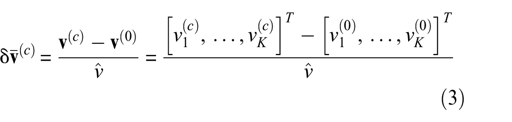
where
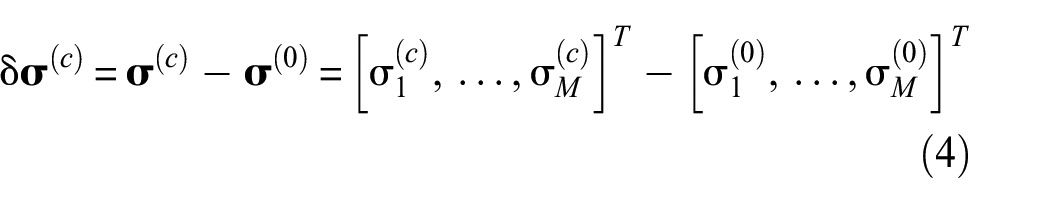
Given a cracked condition of the conductive body, represented by a conductivity distribution
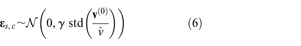
To improve the robustness of the DNN, jitter
46
is included in the training dataset as Gaussian white noise, added to the elements of
with
where
Quality assessment of the training set
Consider now a matrix
In this application, the voltage space is K-dimensional, where each dimension is represented by an interrogated electrode couple. The objective of this section is to define a simple procedure to understand if the distributions of
Due to the high-dimensionality of the problem, visualizing the distribution of real and synthetic measures may be challenging. SOMs 48 can be used to represent the space spanned by the voltage measurements in a human-friendly, low-dimensional representation. Based on this representation, this section also proposes a correlation coefficient that quantifies the similarity between the real and synthetic datasets.
SOMs are unsupervised learning tools that operate through two steps, consisting of (1) a training phase and (2) a mapping process of input data in a low-dimensional (generally, two-dimensional) space. In the first step, competitive learning is employed to find the intrinsic structure of unlabeled input data.
49
In this application, a SOM is trained using the
Without loss of generality, consider a competitive layer formed of a square grid (also called “map”) of neurons with a size of
where
where
After the training process is concluded, one of the most popular approaches to depict the distribution of input instances in 2D consists of representing all the neurons of the SOM as a regular grid with hexagonal mesh,
51
where each link has a color proportional to the Euclidean distance between the neuron weights. Moreover, new voltage instances (or even the ones used for training) can be classified by the trained SOM. The classification process consists of associating each instance to the closest neuron (i.e., its BMU). It is also possible to build a “topological matrix” or “sample hit matrix”
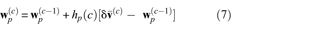
Let
where
The correlation coefficient can also be used to choose between different synthetic datasets obtained using different strategies. For instance, considering H different synthetic datasets, the optimal one to train the network for a specific application can be selected as the one with maximum
Proposed strategy to select the optimal synthetic training set.
Crack identification using DNN
After generating a training set with a high correlation with real data, the DNN can be trained and used to predict the conductivity distribution associated with real voltage measurements collected during future inspections. A DNN with three fully-connected hidden layers, each containing N neurons, in addition to the input and output layers (having K and M neurons, respectively), was employed in this study, as schematized in Figure 2. After the input layer (here indicated as
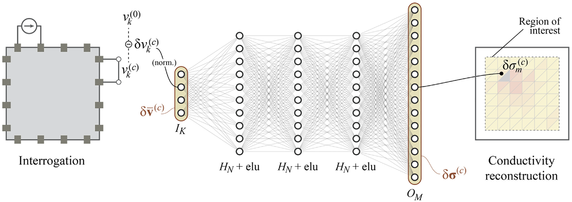
Scheme of the proposed ML-based method to solve the ERT inverse problem.
After training the network, a prediction of the conductivity variation in the inspected body
Experimental investigation
This section presents the results obtained using the proposed framework to solve the inverse ERT problem in four specimens fabricated with two different techniques, the first based on multi-walled carbon nanotubes (MWCNTs) and the second based on GNS. Two different nanocomposite sensing films were prepared to demonstrate that the proposed approach is not confined to a particular type of self-sensing material.
Experimental setup
The sensing layers were fabricated by depositing piezoresistive (i.e., MWCNT or GNS-based) thin films on substrates consisting of polyethylene terephthalate (PET) sheets. PET was selected as the substrate material only for convenience. Since this study aims to investigate the accuracy of EIT in detecting and localizing discontinuities in the piezoresistive sensing film, this choice does not substantially affect the experimental results.
The procedure to fabricate the MWCNT thin film consists of mixing 0.339 g of MWCNT (with an outer diameter of 8 nm (NanoIntegris)) and 0.806 g of N-methyl-2-pyrrolidinone (Sigma-Aldrich) with 33.855 g of 2 wt% poly-(sodium 4-styrenesulfonate) (PSS) solution (which is obtained by dissolving the PSS (Sigma-Aldrich) into deionized (DI) water). The mixture was then immersed in an ice bath and subjected to high-energy tip ultrasonication (5 s on and 5 s off; 6.35 mm tip; 30 min at 30% amplitude) for 1 h to disperse the MWCNT. Then, an appropriate amount of latex solution (Kynar Aquatec) and DI water was added to the MWCNT dispersion to generate sprayable ink. This MWCNT ink fabrication process is described in detail by Wang and Loh. 53
On the other hand, the GNS-based ink was fabricated according to the process described by Lin et al. 40 and is briefly reported herein. GNS, synthesized using water-assisted liquid-phase exfoliation, 54 was added to ethyl cellulose (EC) solution and subjected to bath sonication to disperse the GNS properly. Then the mixer was heated to 60°C and stirred for 12 min to make a sprayable ink.
The MWCNT-latex ink and GNS–EC ink were manually sprayed onto four 108 × 132 mm2 PET substrates (two for each sensing material) using a Paasche airbrush. Each specimen was air-dried at room temperature for at least 12 h before use. After the thin film was completely dry, electrodes were attached along the boundaries of the specimen using copper tape strips. Colloidal silver paste (Ted Pella) was applied over copper tapes to reduce the contact impedance. A total of 18 electrodes arranged in a 4 × 5 pattern were deployed. The fabrication procedure of the specimens is illustrated in Figure 3.
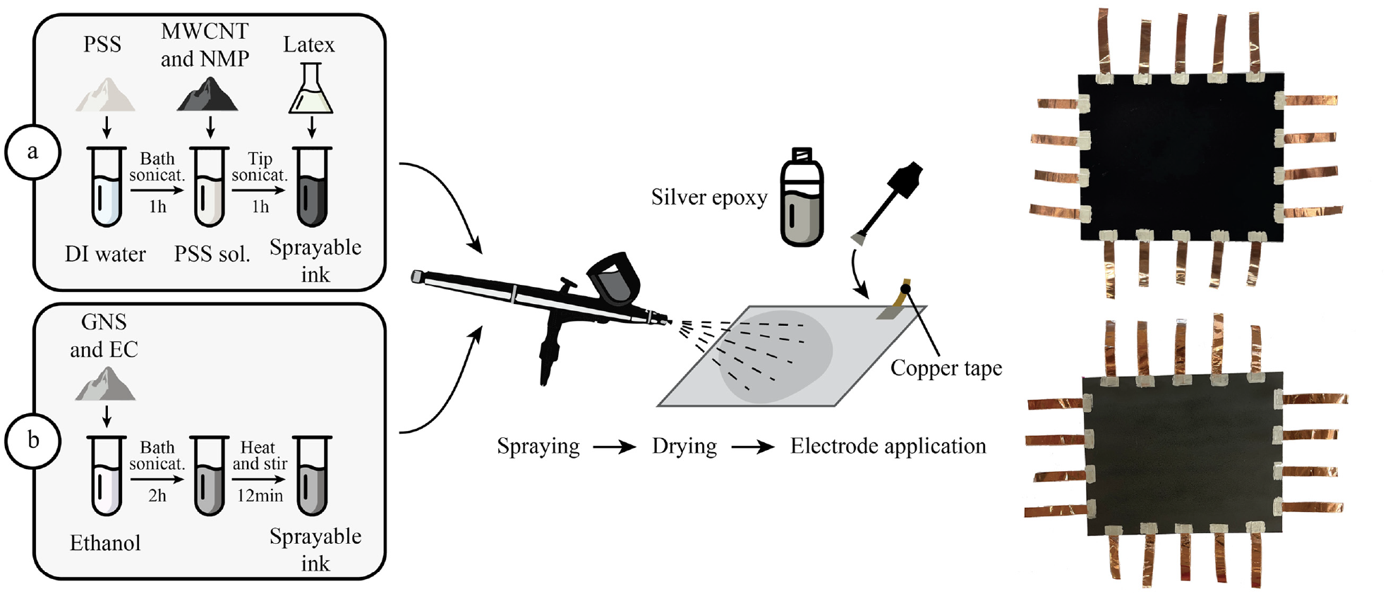
Fabrication process of the specimens: (a) MWCNT- and (b) GNS-based sensing films.
A razor blade was used to cut the specimen to simulate cracking of the substrate (which represents a structural component coated by the sensing film). The crack conditions reported in Figure 4 were induced on the four specimens (each line of the figure represents a different specimen, while each column is a different damage condition obtained by cutting more material along the red lines). Pictures of the experimental setup and an example of a crack are reported in Figure 5. Since PET sheets are flexible, the specimen and the electrodes were fixed on the table using an electrical insulating tape.
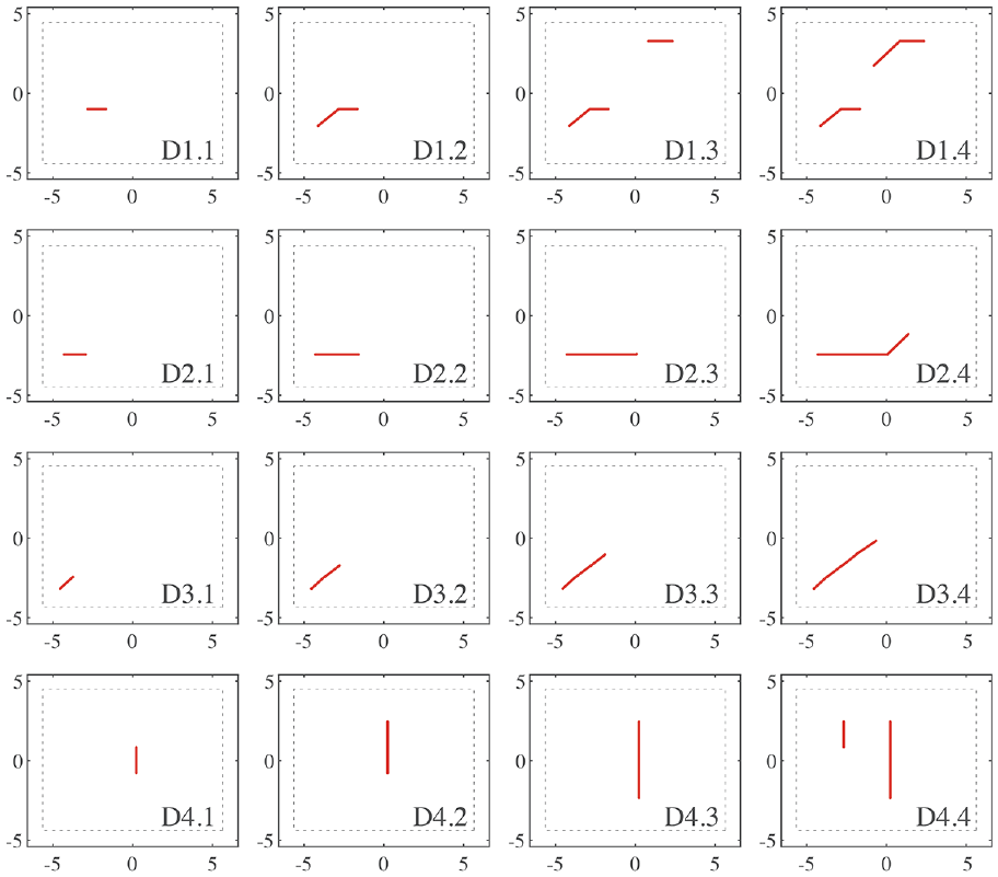
Crack patterns induced in the four specimens.
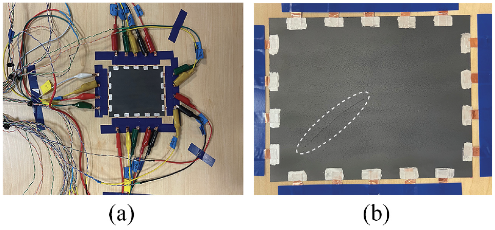
Laboratory test: (a) experimental setup and (b) simulated damage.
For each specimen, a baseline voltage measurement was taken before inducing the damage, when the specimen was intact. After each damage, a new voltage dataset
Selection of the synthetic dataset for training
A FE model of the sensing specimens was built with a triangular mesh structure, as depicted in Figure 6. Then, two different synthetic datasets were generated according the procedure explained in Section “Preparation of the training dataset.” The first dataset was built by considering single and multiple polygonal defects, with random shapes and positions in the region of interest, where conductivity was reduced by a random factor (0%–100%). More details about data generation for polygonal defects can be found in Quqa et al. 55 The second dataset was generated considering randomly distributed line-shaped regions with zero conductivity in the sensing surface. Specifically, a crack was modeled as a random number of connected segments (between 1 and 10) with random length (max 2 cm) and inclination. The position of the crack was also randomly selected within the region of interest of the FE model. The triangular elements of the mesh touching this line were considered as damaged. Two examples taken from these two datasets are shown in Figure 7, where the input (measured voltage difference) and output (conductivity variation in the region of interest) of the inverse problem are represented. In the output, the regions with reduced conductivity are represented with a color proportional to the conductivity variation (according to the color bar on the right of the figures).
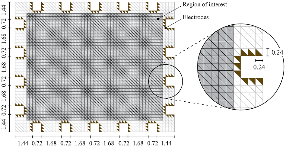
Finite element model of the sensing specimens. Dimensions are in cm.
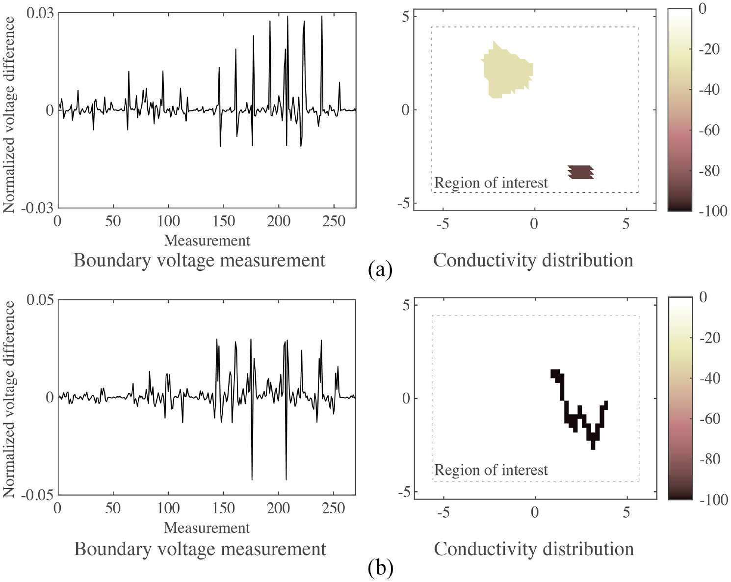
Two examples from the synthetic datasets built for training, consisting of pairs of conductivity distribution and related voltage measurement: (a) polygonal defect and (b) crack-like defect. Axis dimensions in the conductivity distributions are in cm.
Using the four specimens described in Section “Experimental setup,” 16 voltage datasets were collected under different damage conditions (see Figure 4), organized in column vectors
First, this study investigated which of the two synthetic datasets was more suitable to train a DNN to reconstruct the conductivity variation associated with the real voltage measurements. To this aim, the process described in Figure 1 was applied, using SOMs to calculate the correlation factor
Two examples of SOMs trained using the two complete datasets are reported in Figure 8(a) and (b) using a representation style typical for SOMs. 51 The neurons of each SOM are represented in 2D as a regular grid of hexagons. In this representation, the yellow-red colors denote the Euclidean distance between couples of connected neurons. Specifically, yellow indicates close neurons, while dark red denotes large inter-neuron distances. Thereby, yellow areas denote highly populated regions in the K-dimensional voltage space, while red areas signify remote regions.
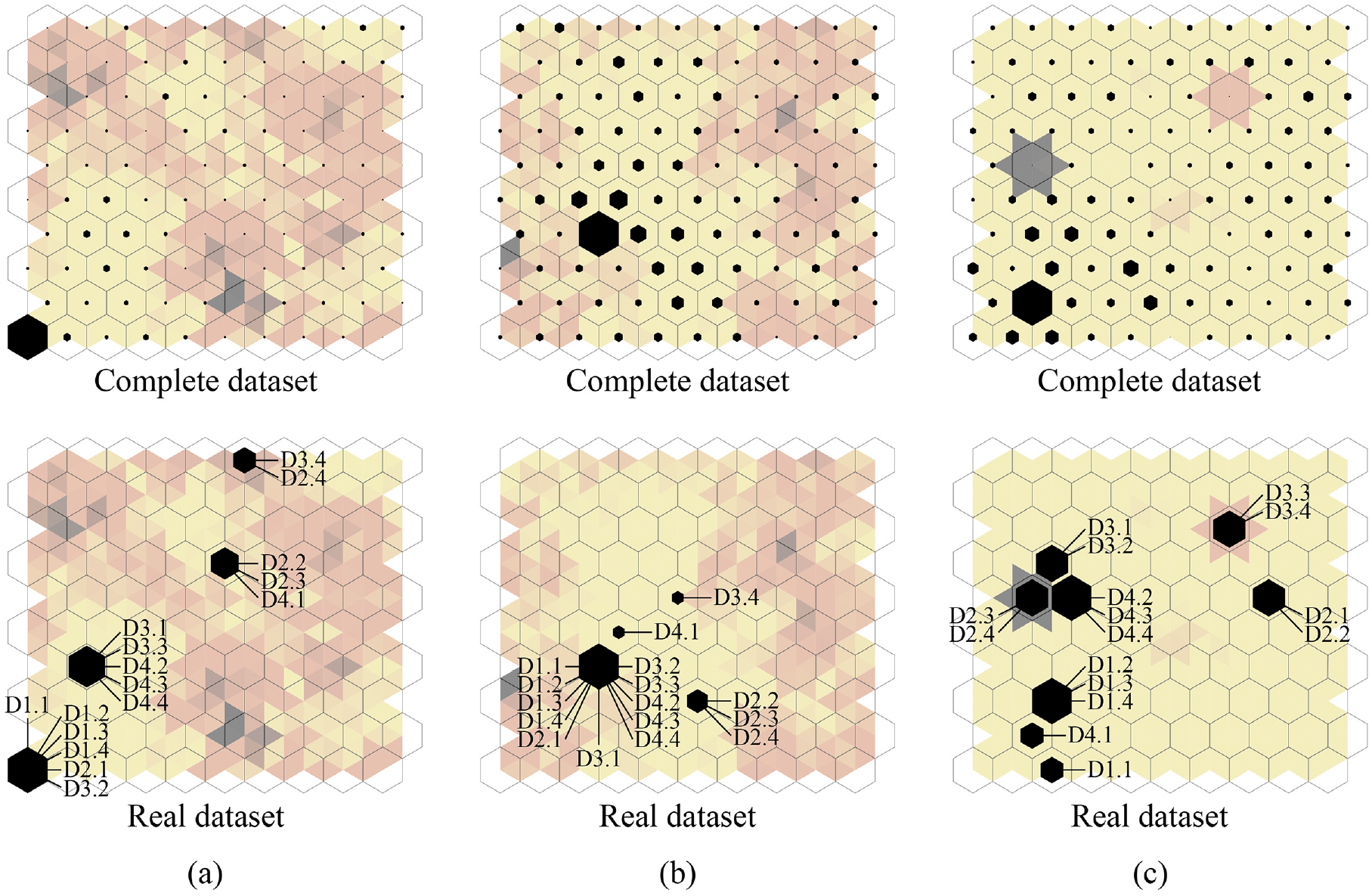
(a) SOMs obtained for polygonal defects with normalized voltage data, (b) crack-like defects with normalized voltage data, and (c) crack-like defects with non-normalized voltage data; the size of full black hexagons is proportional to the sample hits of synthetic (top figures) and real (bottom figures) voltage data.
The full black hexagons have a size proportional to the sample hits of the synthetic (top figures) and real (bottom figures) datasets, that is, the number of instances classified in each neuron from the synthetic and real portion of the training datasets, respectively. In Figure 8, the bottom figures also indicate the detailed classification results obtained using the instances of the real datasets (with reference to the crack patterns schematized in Figure 4). Since the real dataset is much smaller than the synthetic one for lack of real recordings, some neurons are empty in the bottom figures (i.e., they do not classify any real measurements). It should be noted that the real instances are the same for the two cases reported in Figure 8(a) and (b). However, a different structure of the SOM can lead to a different sample hit map.
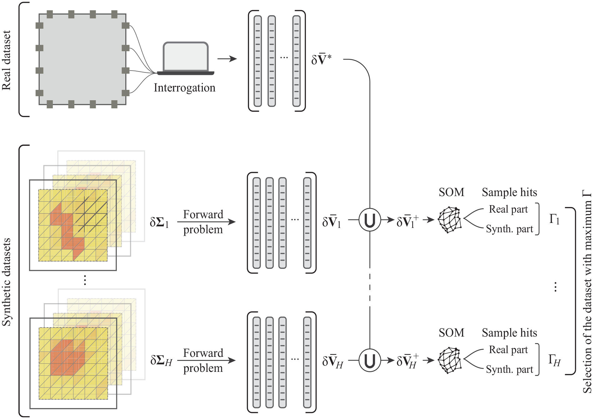
The sample hit distributions of the synthetic and real datasets, normalized with respect to their maximum values, can be compared by calculating the correlation coefficient reported in Equation (9). As previously mentioned, the correlation coefficient quantifies the similarity of the input space structure between a synthetic and a real dataset, that is, it measures the overlap of the instance distribution in the K-dimensional space. This measure is indicative of the suitability of a synthetic dataset to train a supervised ML tool able to predict the real instances. 47 The average correlation coefficients calculated on 100 different SOMs are 0.7871 and 0.9245 for the datasets obtained for polygon and crack-like defects, respectively. These results indicate that the structure of the synthetic dataset representing crack-like defects is more similar to that of the collected voltage measurements.
It is worth noting that the normalization performed in Equation (3) is fundamental since training the SOM with non-normalized data would lead to the result reported in Figure 8(c), where synthetic and real data populate different regions of the voltage space. Indeed, two remote spots in the SOM are clearly visible (in dark red), which only include real instances. In the case of non-normalized data, the average correlation coefficient calculated on 100 SOMs would be only 0.1943, representing a training dataset that is poorly effective in predicting the real instances.
While data normalization proved essential to maximize the generalization capabilities of the network, this approach does not allow for a physical quantification of conductivity variation. Furthermore, the batch normalization layer of the network (see Section “Crack identification using DNN”) also affects the quantification ability but was fundamental in this study to obtain consistent results. The issue of data normalization will be further addressed in future works.
Discussion of the results
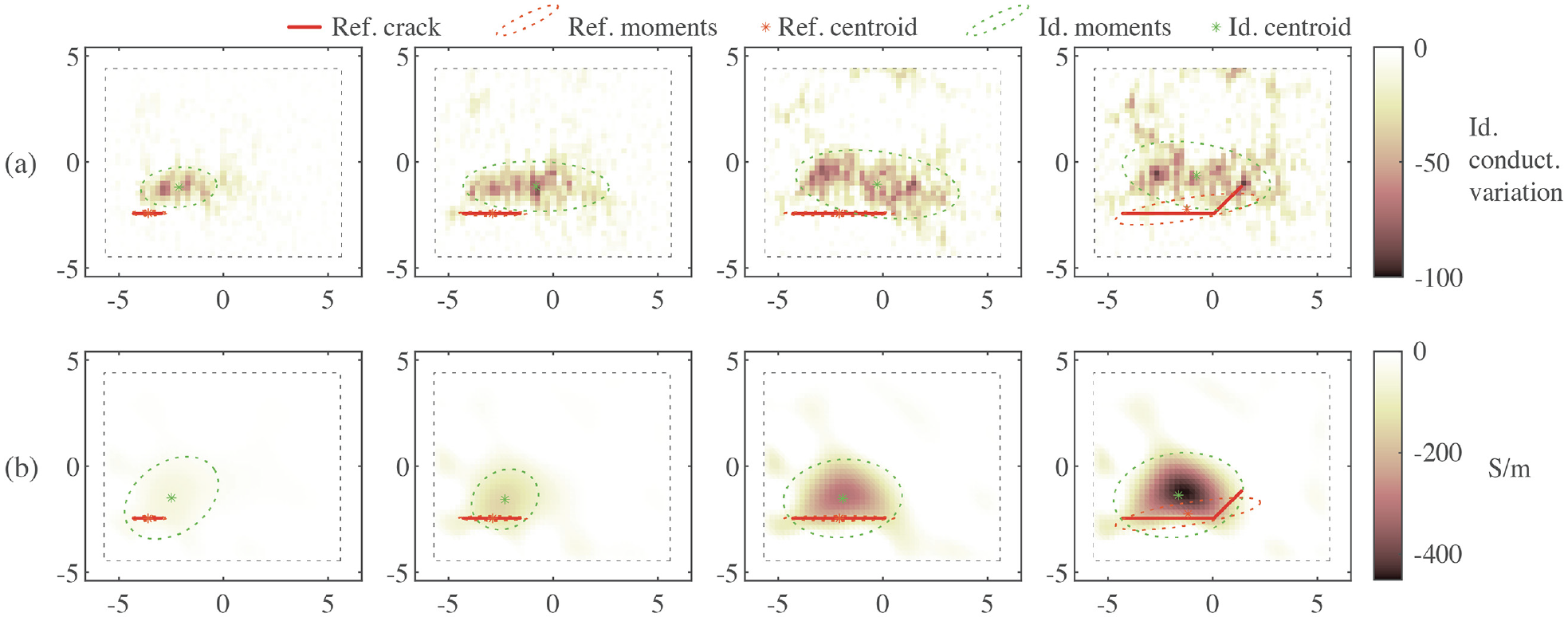
The normalized synthetic dataset representing crack-shaped defects was thus used to train a DNN employed to reconstruct the conductivity distributions associated with the real voltage measurements collected from the four specimens described in Section “Experimental setup.”Figures 9 and 10 show the reconstructed conductivity distributions corresponding to the damage states induced by cutting the two MWCNT-based sensing specimens using the razor blade in the highlighted locations (red lines). Specifically, Figures 9(a) and 10(a) plot the results obtained using the presented ML-aided method. Here, the values in the color bar (0–100) are representative of a dimensionless conductivity reduction associated with the normalized voltage measurement. For comparison purposes, Figures 9(b) and 10(b) show the results obtained with the TV method, using a weight equal to 10−6 for the regularization matrix. 28 Conductivity was reconstructed in a region of interest (dashed rectangle, 88 × 112 mm2) slightly smaller than the specimen itself (solid rectangle, coinciding with the axes of the figures, 108 × 132 mm2). The reconstruction was limited to this reduced area to avoid inaccuracies due to the modeling assumptions of the boundary region.
Conductivity distribution reconstructed for Specimen #1 through (a) the ML-aided approach and (b) the TV method. Axis dimensions are in cm.
Conductivity distribution reconstructed for Specimen #2 through (a) the ML-aided approach and (b) the TV method. Axis dimensions are in cm.
These two figures show that small cracks are generally correctly identified in both specimens. Concerning the ML-aided approach, as the crack size increases, a higher noise amount populates the reconstructed conductivity distribution. Also, the shape of multiple cracks cannot be properly recognized since the defect is reconstructed as a single connected region with low conductivity. Nevertheless, an approximate estimate of crack extension and location can always be identified. Besides, the magnitude of identified conductivity reduction is almost constant for the different damage cases, allowing easy identification of small defects. On the other hand, the shape of the damaged regions identified using the TV method is very similar between the different damage cases of the same specimen but only changing in magnitude. This result makes understanding how damage is evolving particularly challenging.
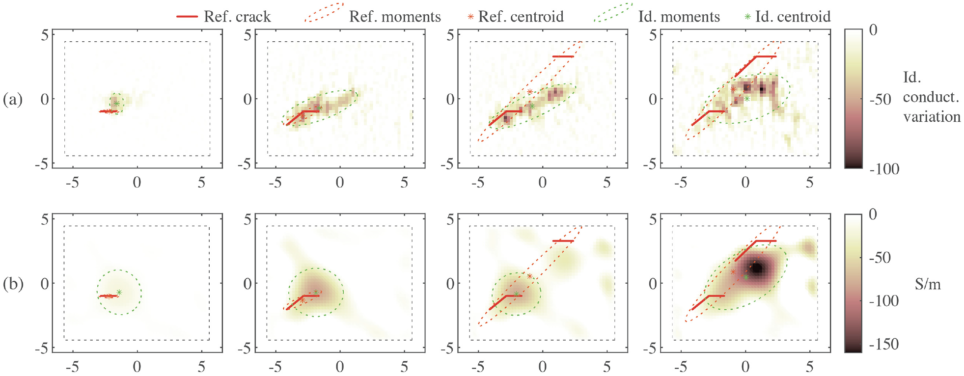
As in the previous cases, Figures 11 and 12 show the reconstructed conductivity distributions obtained using GNS-based specimens. In general, a less-detailed reconstruction of the conductivity distribution is identified. Considering Specimen #3, small defects are well localized and quantified (in terms of size) using the ML-aided approach. Although the direction of the reconstructed crack is slightly different from that of the reference damage, the crack extension and location are well approximated. On the other hand, the results obtained using the TV method represent the damage magnitude but do not provide accurate conductivity reconstructions. Considering Specimen #4, the small crack in the first damage state is not identified by any of the two methods. This result may be due to the selected interrogation pattern. Indeed, it is well known that the Sheffield measurement protocol is generally more sensitive to conductivity variations close to the boundary of the interrogated specimen. 45 On the other hand, an “opposite” 56 interrogation pattern would be more sensitive to conductivity variations in the central sensing region as the current travels more uniformly through the imaged body and is less sensitive close to the boundary. 45 Different interrogation patterns will be investigated in future research. Using the TV method, the second and third crack evolutions in Specimen #4 are identified as a conductivity reduction that increases in magnitude as the crack size grows. The conductivity distribution reconstructed using the ML-based method in the last two scenarios also presents a wider low-conductivity region in the middle of the sensing area; however, the two cracks of the last damage case are not clearly distinguishable.
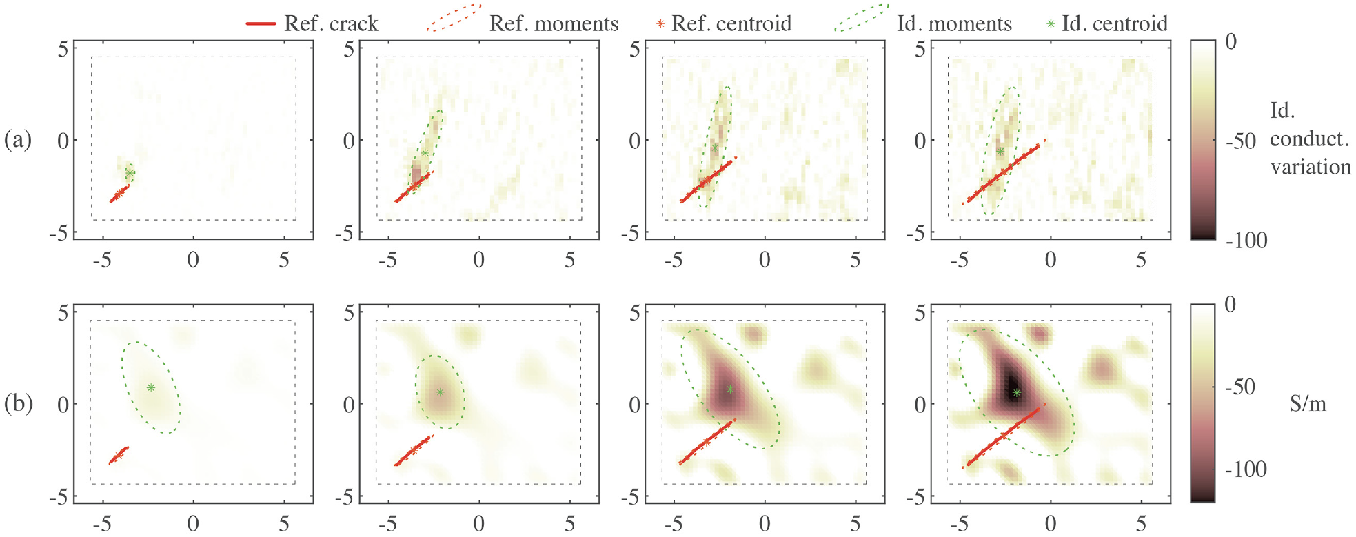
Conductivity distribution reconstructed for Specimen #3 through (a) the ML-aided approach and (b) the TV method. Axis dimensions are in cm.
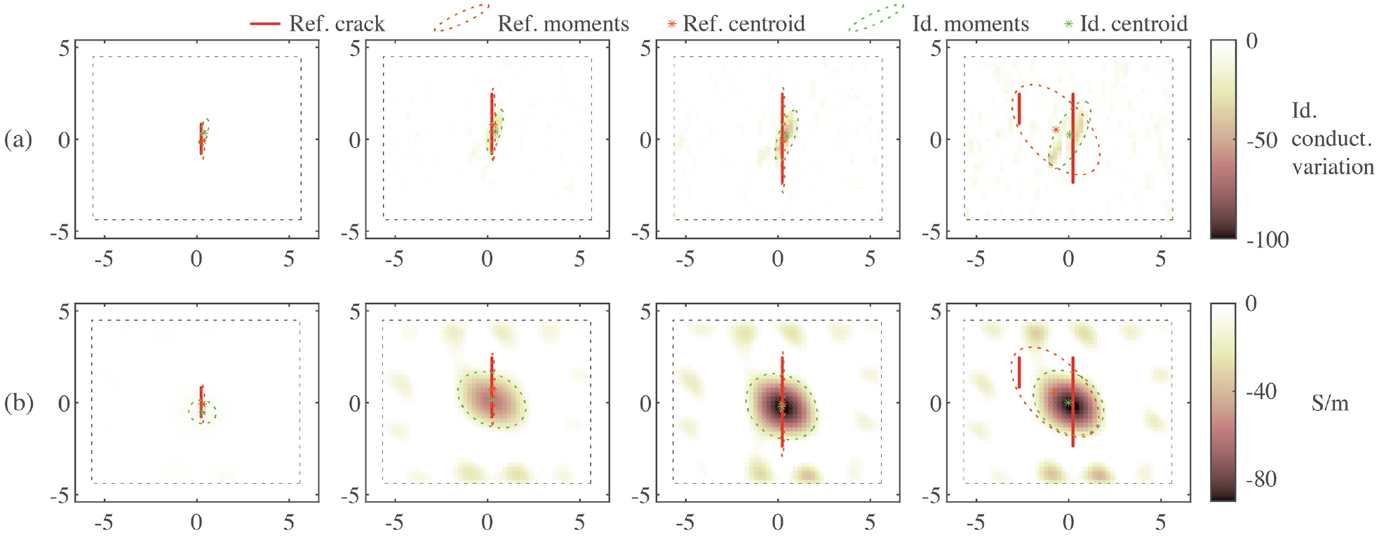
Conductivity distribution reconstructed for Specimen #4 through (a) the ML-aided approach and (b) the TV method. Axis dimensions are in cm.
Identification accuracy was also quantified using the following procedure. First, for each test (including reference cracks, ML results, and TV results), a region was calculated that included all the areas where the conductivity variation was higher than 10% of the maximum (identified or reference) conductivity variation. This process was used to exclude artifacts. Then, the centroid and the second moments (with respect to principal axes) were calculated for the identified regions. An ellipse that has the same second moments as the identified regions was thus drawn (dashed lines in Figures 9–12).
Three indicators were used to quantify the identification accuracy: (1) the Euclidean distance between the centroids obtained for the reference and the identified regions, (2) the percentual difference between the largest diameters of the ellipses of the reference and identified regions, and (3) the rotation between the largest diameter of the identified ellipses (in absolute value). These quantities are reported in Figure 13 for each test. The average parameters among all tests are also indicated with dashed horizontal lines. The three parameters employed for accuracy assessment are representative of (1) the localization, (2) the entity (in terms of size), and (3) the orientation of the cracked region, respectively. The third parameter may be particularly useful to connect the identification result to a particular physical phenomenon that generated the crack (e.g., due to shear vs flexural state) or to predict the next steps of crack propagation.
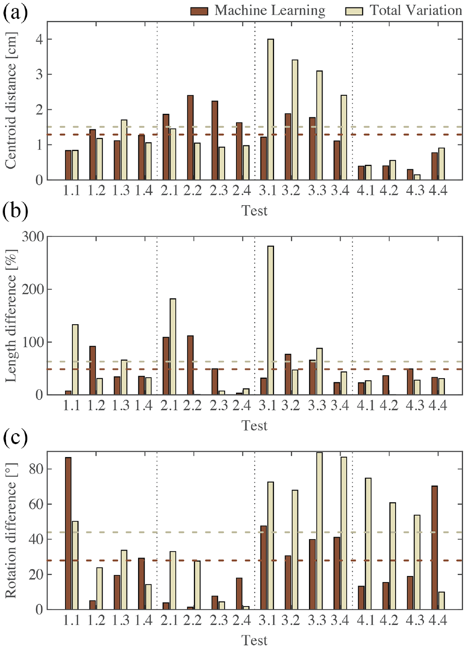
Performance indicators: (a) Distance between identified and reference centroids, (b) percentual difference between identified and reference maximum diameters and (c) absolute rotation difference between identified and reference maximum diameters. Average values are reported as dashed lines.
While identification accuracy is overall comparable between ML and TV in terms of the size of the cracked region, identification of crack orientation is considerably improved with ML (28° vs 44° difference on average). Another benefit of the ML process is the short runtime, which was two orders of magnitudes lower than the runtime of a single iteration of the TV method, that is, 0.6 vs 0.006 s using MATLAB (R2020b version) running on an Intel® (Santa Clara, California, United States) Core™ i7-8,700 6@3.20 GHz-processor CPU with 2 GB NVIDIA (Santa Clara, California, United States) Quadro P620 GPU, 32 GB RAM and Windows 10 operating system .
This study was conducted to investigate the usability of EIT to identify and localize disconnections in the sensing layer, that is, the deposited piezoresistive paint. EIT has also shown to be effective in detecting strain states. 55 Embedded cracks near the free surface (e.g., delamination) or small cracks due to a tensile state may not involve disconnections in the sensing film. However, in general, they generate a variation in the surface strain, which changes the conductivity of the sensing film. This change can be detected if the entity of the resulting surface dilation is significant.
Conclusions
This work presented the results obtained by solving the ERT inverse problem to reconstruct the location and extension of cracks in a thin sensing film employed for SHM. Specifically, a DNN was trained using a synthetic dataset generated by solving the forward problem through a FE mesh model. The suitability of the training set for practical applications involving real voltage measurements was validated using a novel procedure proposed in this work. In particular, a correlation coefficient that measures the similarity between the high-dimensional voltage space populated by real measurements and that populated by the generated synthetic data was calculated. Comparing this coefficient obtained for different synthetic training datasets allows deciding which one is the most representative for the specific application in which real data is collected. This coefficient is simple to calculate and does not necessitate any prior information on the damage location. Therefore, it can be calculated after collecting voltage measurements directly taken from the experimental campaign. Moreover, the method enables a conscious evaluation of the suitability of the generated training dataset, which is generally a challenging aspect when applying supervised ML tools for real applications.
After training the network with the most suitable dataset, the conductivity distribution was reconstructed for different damage conditions induced in four rectangular sensing specimens tested in the laboratory environment. The results showed that, in general, small cracks are accurately identified using the presented ML-based method, both in terms of size and location. As the damage size increases, the reconstruction becomes noisier. However, an approximate location, orientation, and entity of the cracked area can still be identified. On the other hand, the TV method provided conductivity distributions with less accurate defect shape, reflecting the crack entity in terms of conductivity magnitude. In general, tests conducted on the CNT- and GNS-based specimens show similar performances. Moreover, slight damage involving the central part of the sensing region is identified less accurately as compared to cracks investing boundary areas, probably depending on the current injection pattern employed for interrogation.
The performance of conductivity reconstruction strongly depends on the similarity between the instances of the training dataset and real voltage measurements. Therefore, further research needs to be conducted to make the training dataset as representative as possible of the real measurements, while keeping the complexity of the model contained.
Footnotes
Declaration of conflicting interests
The author(s) declared no potential conflicts of interest with respect to the research, authorship, and/or publication of this article.
Funding
The author(s) disclosed receipt of the following financial support for the research, authorship, and/or publication of this article: This research was partially supported by the U.S. Army Corp of Engineers, Engineer Research and Development Center (principal investigator: Prof. Michael D. Todd), under Cooperative Research Agreement W912HZ-17-2-0024 and W9132T-22-2-20014. Additional funding was also provided by the University of California San Diego, Jacobs School of Engineering. Mr. Said Quqa (working under Ph.D. advisor Prof. Luca Landi), and his visiting scholar appointment at UC San Diego and the ARMOR Lab, was supported by the University of Bologna, within the Marco Polo program.