
Abstract
In order to reconstruct the possible defects on the plate surface with arrays, a new wave tomography method based on the method of moments is established in this paper. According to the relationship between the probe number and grid amount, two algorithms, that is, the neural network and principal component analysis (PCA), are proposed and used to solve the ill-conditioned inversion equations. The neural network makes imaging feasible even if input data are not enough, and the PCA can greatly improve the computational efficiency via reducing the matrix dimension. Both numerical simulations and experimental measurements are conducted with the algorithm’s correctness and high precision validated. After investigating the influence of probe number on imaging quality, it is demonstrated that the algorithm can exactly predict the defect location when the input scattering data is not enough or fewer probes are arranged. More probes are needed for reconstructing the specific shape and thickness, especially when multiple defects are included. The qualitative results and quantitative data are conducive to providing some reference for engineering applications in nondestructive testing and structural health monitoring.
Introduction
Lamb wave, a type of guided wave in plates, has become one of the hotspots in the field of nondestructive testing (NDT) and structural health monitoring (SHM) regions because of its long propagation distance and dispersive feature.1,2 The wave velocity is related to the plate thickness, and then can be utilized for detecting corrosion defects.3,4 Taking the A0 mode for example, it is very sensitive to the plate thickness when the value of fh is small. Here, f and h are the working frequency and plate thickness, respectively. Therefore, it is viewed as the priority when detecting surface defects. Additionally, it is more easily generated and received than bulk acoustic waves,5–7 and then plenty of methods based on the A0 mode have been developed for NDT.
During the method development, the algorithm plays an important role in final defect visualization, which is directly related to the quality of final imaging. The defect profile is required to be reconstructed after utilizing a proper algorithm based on the wave amplitude,8,9 phase,10,11 wave number,12,13 and other related characteristics of received signals from transducers. Therefore, how to develop a new algorithm and establish an accurate mathematical model to realize the qualitative and quantitative analysis according to different conditions, is of great significance for NDT or SHM.
Generally, typical algorithms for defect reconstruction include the elliptic imaging algorithm,14,15 rapid imaging algorithm,16,17 intelligent evolutionary algorithm,18,19 etc. They are mainly interested in the macro-information carried by the signal from transducers, including time-of-flight and amplitude. Normally, these algorithms converge quickly and are suitable for judging the defect location. However, the imaging accuracy is not satisfactory, especially when identifying the defect profile using sparse arrays of transducers. In order to improve the resolution, the annular array with more probes is proposed and developed, as well as the corresponding algorithms, including diffraction tomography,
20
HARBUT algorithm,
21
full-waveform inversion,
22
and so forth. These algorithms are derived from the basic acoustic governing equations, in which the scattering mechanism of defects is considered. Mostly, the imaging resolution is satisfactory. However, enough data must be inputted when using these algorithms, and the transducer number N in an annular array must satisfy
In this paper, a reasonable inversion model is established by using the method of moment (MOM).24–26 The highlight is that two algorithms are proposed according to the probe number arranged and the grid amount in the detection region. After that, the influence of different probe numbers on the imaging results is investigated in detail. When the equation is underdetermined, the corresponding neural network is designed, which can update the weight through the feedback of errors. 27 After inversion, the underdetermined equation is simplified into a single-layer neural network model and the network weight can achieve a good convergence. For overdetermined problems, the principal component analysis (PCA) is developed, 28 which can reduce the data dimension and efficiently improve computational efficiency. Additionally, PCA can also coordinate the main components, remove noise interference, and reduce the error to the greatest extent.
Firstly, the inversion equation is established based on MOM in “Design of tomography algorithm”, and the corresponding algorithms are introduced systematically, including the design scheme, convergence criterion and data processing. After that, numerical simulations are carried out with the aid of ABAQUS in Section “Numerical model and results.” The wave signals obtained are implanted into previous algorithms, and the defect reconstruction is shown. Utilizing the two algorithms, the influence of probe number on imaging quality is illustrated visually. In order to furthermore validate the algorithms, experimental measurements are conducted in Section “Experimental model and results,” which is based on a self-designed air-coupled system. Finally, some conclusions are summarized in Section “Conclusion.” It is expected that the algorithms developed in this paper can provide technical guidance for NDT or SHM technologies.
Design of tomography algorithm
Basic model
It is assumed that a circular area surrounded by dotted lines in the middle of a blue rectangular plate in Figure 1 is the detecting region, around which eight transducers are set at the same angle. If a two-dimensional Cartesian coordinate system is established at the circle center, the coordinate positions of all sensors can be obtained when the probe number and the radius are known. One transducer is used for wave generation and the others are receivers. Then, transform the emitting probe one by one and repeat the above process, the scattered field can be captured. This is a typical arrangement of sparse arrays when detecting defects inside the circle. Generally, more probes can produce better imaging results. Several array patterns, such as 16, 32, and 64 arrays with the same angle of configuration, can be designed to meet different requirements of detection. However, how to efficiently solve the governing equations and realize the defect reconstruction for any arrays, is challenging. It is anticipated that the present contribution can provide some guidance on this issue.
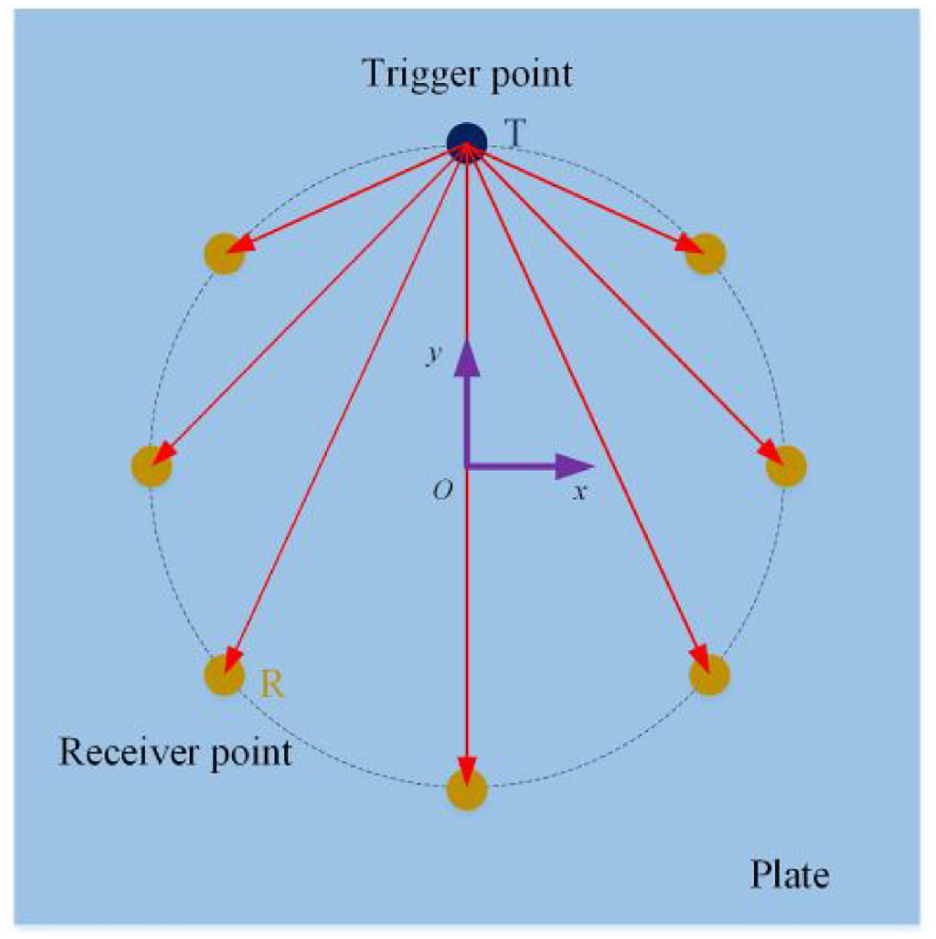
Schematic diagram of a basic detection array.
In this paper, a single A0 mode with a frequency f is utilized for NDT. Because of dispersion, the phase velocity of A0 mode is dependent on the plate thickness if the working frequency is fixed. Then, the defects in the plate can be expressed indirectly with the aid of phase velocity. In the following sections, the guided wave tomography will be adopted here to reconstruct the phase velocity distribution in the unknown area and then convert it to thickness, so that defects can be detected visually. It should be stressed that the scattering waves with more modes can be generated if the defect boundary changes drastically. 29 However, there is no mode conversion as the thickness varies slowly. 21 Therefore, it is assumed that corrosion-type defects do not lead to mode conversions. In order to illustrate the defect boundary as much as possible, an iterative solution is proposed in this paper with the specific algorithm demonstrated in the next section.
Establishment of the algorithm
The basic idea of this algorithm is to collect the scattering signal
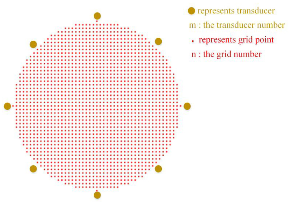
Grid diagram of the imaging area.
Originally, the Lippmann Schwinger equation requires:30–32
in which
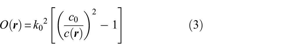
Here,
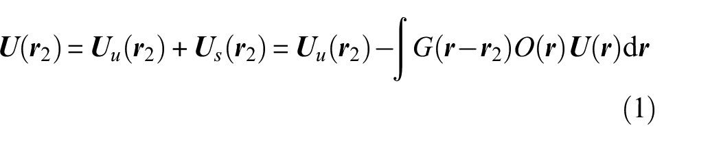
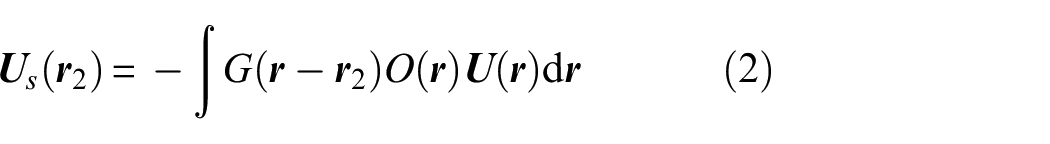
Considering Equation (2) is an integral expression, it is difficult to directly use it to solve the objective function. Based on the grids described above, the corresponding transformation of Equation (1) can be obtained by utilizing MOM:25,26
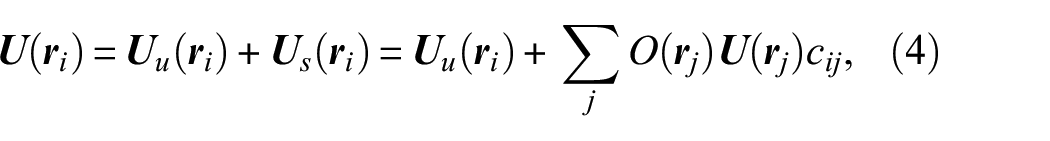
with
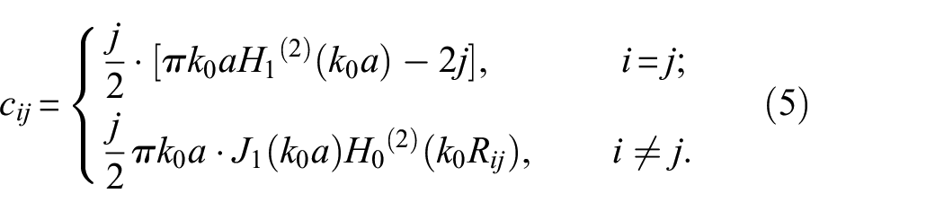
Here
Here,


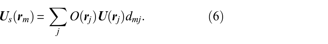
where
Figure 3 is the basic flow of the imaging algorithm in this paper. It also returns to the original problem in this section, that is, how to solve the underdetermined and overdetermined equation when using different arrays, which will be highlighted in the next section.
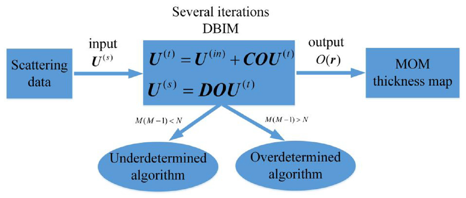
Flowchart showing the stages of iterative imaging algorithms.
Solving algorithm
Before iteration, replace
At the beginning of the iteration, the total field
Therefore, the problem of solving an iterative process can be summarized in a general form:

When Equation (9) is a system of underdetermined equations, the single-layer neural network is developed to iteratively find the stable root. On the contrary, if Equation (9) is overdetermined, PCA is utilized to solve it. The two algorithms will be introduced in detail below.
Neural network for solving underdetermined equations
Let
The weight can be adjusted by the following formula:
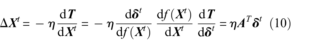
Here

with
PCA for solving overdetermined equations
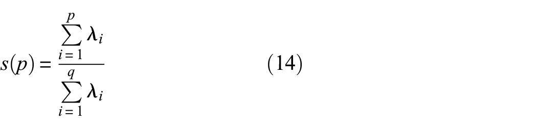
To avoid complex matrix operations, this method does not follow the standard process of PCA. At first, singular value decomposition is performed on

in which
Let

Equation (13) is a formula for finding roots using PCA. Correspondingly,
when
Convergence criterion
Section “Solving algorithm” only describes two methods for solving ill-posed equations but does not provide a convergence criterion for iteration. As defined by relative errors (RE), the following equation can be obtained:

where
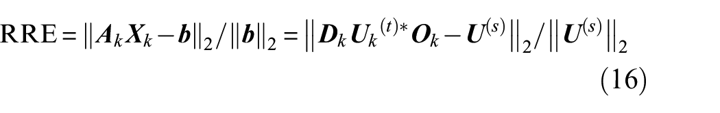
Usually, the iteration is stopped when
Data processing
Equations (7) and (8) of MOM are derived from the primal Lippmann-Schwinger equations, which are calculated in the frequency domain. Therefore, extracting the scattering field in the frequency domain during simulations or experiments plays a key role. The most basic scattering field can be achieved by the following expression:

Here
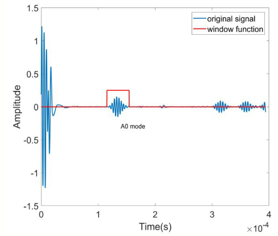
A set of experimental received signals.
In general, the incident field is equivalent to the total field of the non-destructive region. Thus, one method to obtain
in which

Here,
The utilization of Q to calibrate the scattering field is a very important step in the iterative process of inversion, which can reduce the error of simulations (or experiments). Evidently, the above methods of data processing mainly introduce the extraction of the scattering field and the proposal of the calibration factor.
After illustrating details associated with signal processing, the imaging method will be demonstrated. As mentioned above, a combination of experimental and theoretical calculations is used to obtain
Numerical model and results
Numerical model
In order to verify the algorithm, ABAQUS software is utilized to simulate several aluminum plates with different kinds of defects. The plate size is chosen as 1200 mm × 1200 mm × 3 mm, and the diameter for detection is 400 mm. For material parameters, Young’s modulus, Poisson ratio, and density are 70.8 GPa, 0.34, and 2700 kg/m3, respectively. Additionally, several layers of materials with increasing Rayleigh damping coefficients are added around the aluminum plate edges to form an absorption layer,37–39 which are used to fully absorb the reflected wave from plate boundaries. The source excitation is a 5-cycle Hanning windowed toneburst signal at a central frequency of 200 kHz. C3D8R elements are distributed with at least three meshes adopted along the plate thickness direction. Recomputation has been carried out with smaller elements before final simulations, which can make the numerical results convergent and accurate.
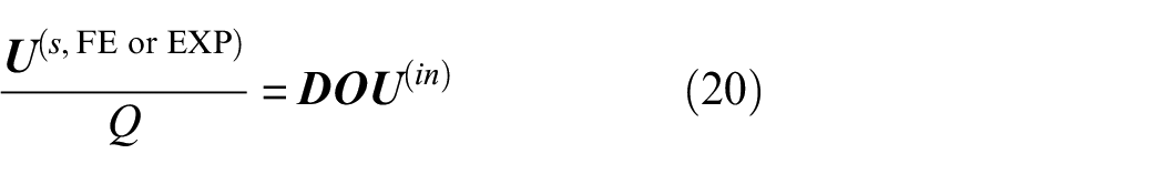
Figure 5 shows the thickness distribution of four theoretical models. Both Figure 5(a) and (b) belong to a single defect model with the defect center at (0, 0). The thickness of the triangular defect in Figure 5(a) is uniform, while the elliptical defect in Figure 5(b) has a gradient change in thickness. Additionally, two defect models are also considered in Figure 5(c) and (d), in which Figure 5(c) has double circle defects with different sizes and Figure 5(d) consists of a triangle defect and an elliptical one.
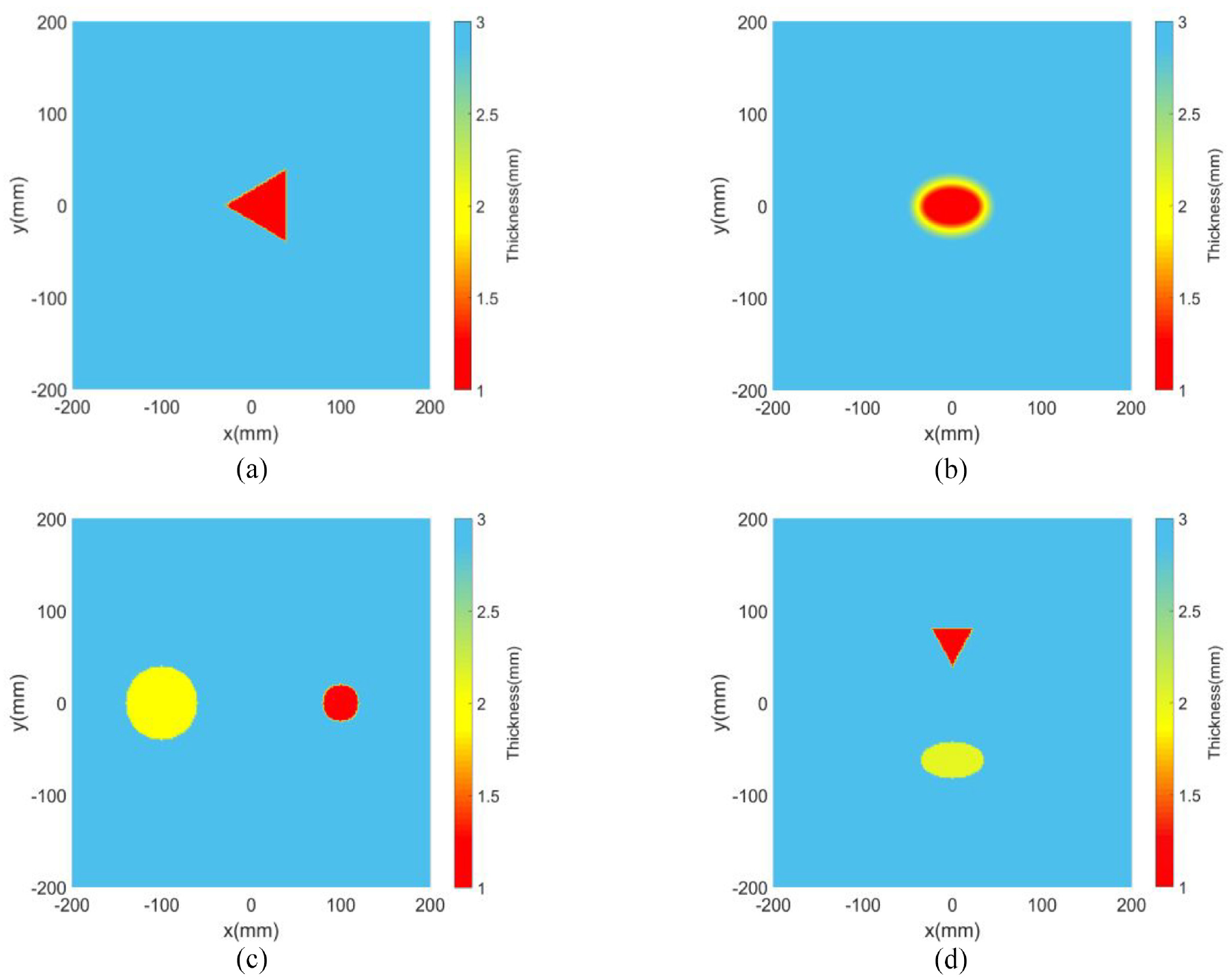
Theoretical models. (a) An equilateral triangle defect locates at (0, 0), and the side length is 80 mm with a remaining thickness of 1 mm. (b) The elliptical defect locates at (0, 0), and the long and short axes are respectively 80 and 40 mm with a remaining thickness of 1 mm. The defect thickness varies smoothly from its edge to the plate. (c) The large circle defect centered at (−100, 0 mm) has a radius of 40 mm and a remaining thickness of 2 mm, and the small circle defect located at (100, 0 mm) has a radius of 20 mm and a remaining thickness of 1 mm. (d) The equilateral triangle defect centered at (0, 60 mm) has a side length of 48 mm and a remaining thickness of 1 mm. The elliptical defect centered at (0, −60 mm), whose long axis and short axis are respectively 70 and 40 mm, the remaining thickness is 2 mm.
Reconstruction results
For detecting the defects in Figure 5, the detection region is divided into 1793 points. The array with 8, 16, 32, and 64 probes are used, respectively. The first three models obtain 56, 240, and 992 groups of input scattering data, respectively, and all of them select the neural network method for iterative solutions. The 64-array case can receive 4032 groups of scattering fields, and the PCA algorithm is selected to avoid noise pollution caused by redundant data. Correspondingly, the reconstruction results are shown in Figures 6 to 9. Meanwhile, to visually evaluate image quality, the thickness distributions across the defect center are extracted and illustrated in Figure 10. By contrast, the theoretical value of the actual defect is also included.

Reconstruction results of the triangular defect by (a) 8-array model, (b) 16-array model, (c) 32-array model, and (d) 64-array model.
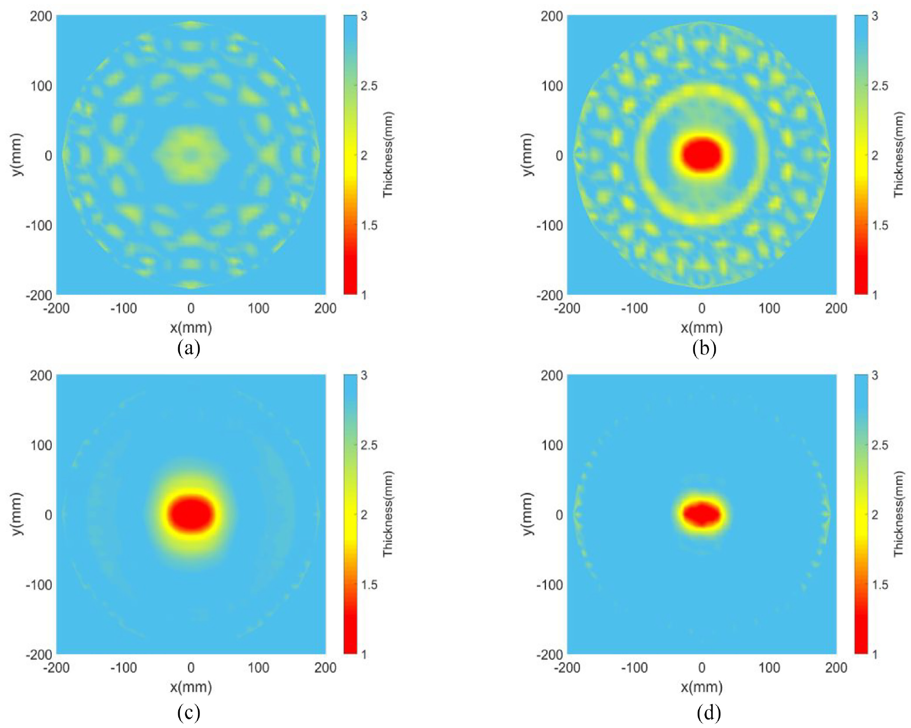
Reconstruction results of the elliptical defect by (a) 8-array model, (b) 16-array model, (c) 32-array model, and (d) 64-array model.
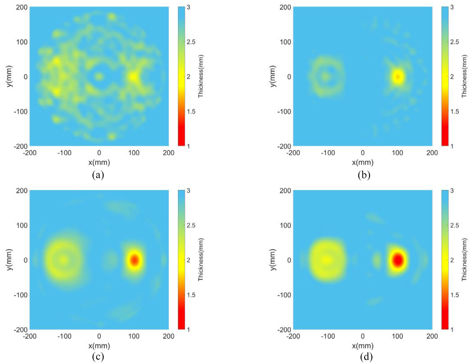
Reconstruction results of the double circular defects by (a) 8-array model, (b) 16-array model, (c) 32-array model, and (d) 64-array model.
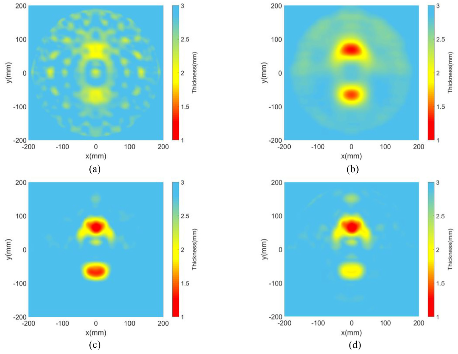
Reconstruction results of triangular and elliptical defects by (a) 8-array model, (b) 16-array model, (c) 32-array model, and (d) 64-array model.
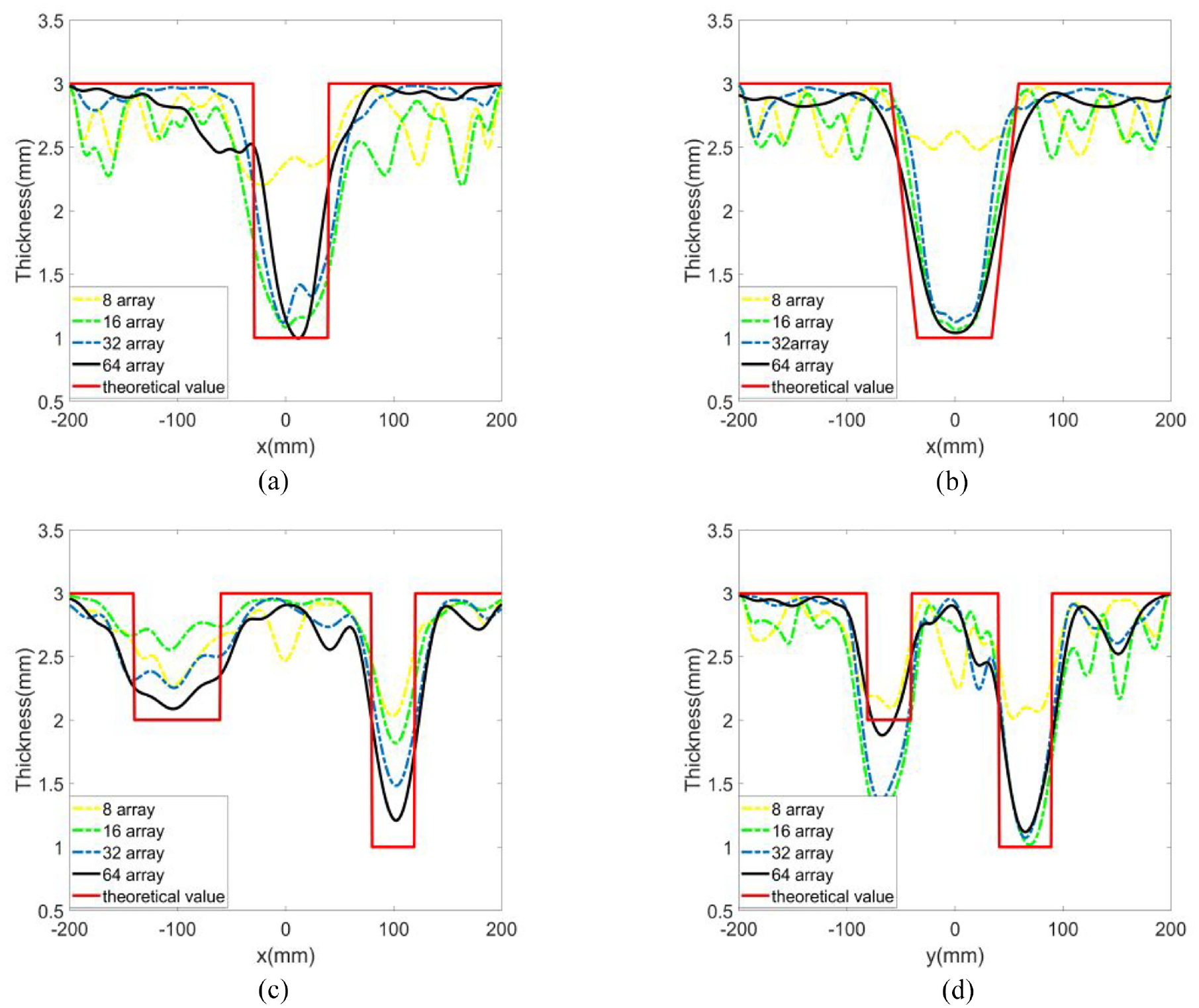
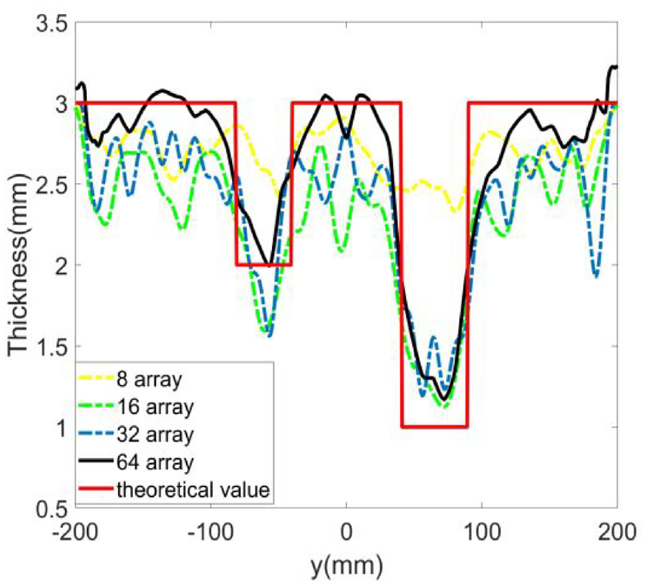
Cross-sections of the thickness reconstructions across the defect center from (a) Figure 5(a), (b)Figure 5(b), (c)Figure 5(c), and (d)Figure 5(d). The yellow, green, blue, and black lines represent the results calculated from the 8, 16, 32, and 64 probes, respectively, and the red solid line corresponds to the actual defect.
From a whole perspective, the reconstruction results of MOM can effectively distinguish the defect location. The shape and thickness information of defects are closer to reality as the probe number increases. The imaging of these four types calculated by eight probes is relatively poor. For single defect such as Figure 5(a) and (b), the 8-array model can only roughly make a distinction between noise and defect. For the two defects, it is even difficult to make a qualitative evaluation with a lot of overlap between the defect and surrounding noise. By contrast, the 16-array model can reconstruct a relatively good imaging, because it can effectively seek the damaged area. From the quantitative reconstruction results in Figure 10(a) and (b), it can be seen that the error is controlled within 0.2 mm for the single defect cases. Unfortunately, it is still not ideal for identifying the defect shape. The neural network method combined with 32 probes is able to conduct a quantitative evaluation in the single defect, with the contour and depth very close to the reality. However, when facing multiple defects with more scattering forms, there are still considerable errors in the reconstruction of thickness. As the probe number further increased to 64, the shape and depth of defects can be reconstructed accurately with the noise pollution at a very low level, and the reconstruction results are best. Totally speaking, Figures 6 to 10 efficiently validate the correctness of the wave tomography method proposed in this paper. It should be stressed that the calculation speed of PCA is fast with only partial principal components being selected to participate. For example, when inputting data from the 64-array is adopted, only less than 3 minutes are needed at a time. Therefore, this method is convenient to be applied in NDT.
Reviewing Figure 10, it also can be concluded that a defect with a small gradient variation along thickness is easier to be reconstructed. For illustrating this, the thickness value on the cross-sections in Figure 10 is extracted and a parameter RNL is defined as
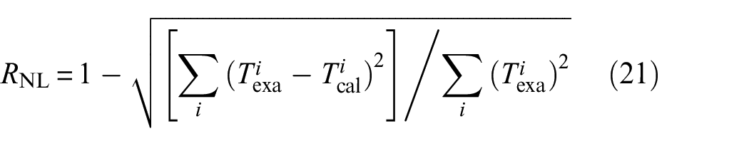
in which
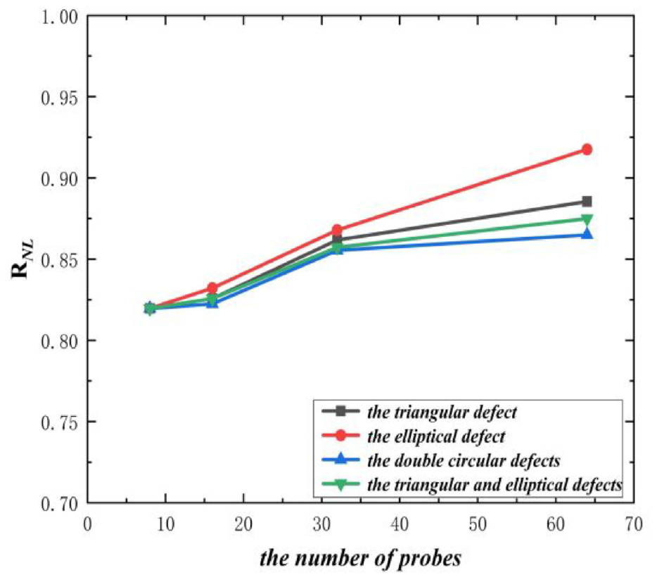
The RNL variation for different defects.
Experimental model and results
Experimental model
For furthermore validating the correctness of algorithms, as well as the influence of probe number on reconstructing different defects, experiments are carried out. An equilateral triangle defect and an elliptical defect that are the same as in Figure 5(d) are fabricated in an aluminum plate, such as in Figure 12. A pair of non-contact air-coupled probes (Japan Probe 0.2 K 14 × 20 N) are designed as transducers, and probes are located at the same position as those in numerical simulations. A 5-cycle Hanning windowed toneburst signal with the central frequency of 200 kHz is chosen as the wave generation, and the excitation and reception are integrated into a set of NDT system (JPR-600C). For eliminating the unnecessary reflected waves, damping glues are attached to the aluminum at plate edges. The air-coupled probes are suspended above the reference points, and the distance between them will be continuously changed to meet different paths of detection. For exciting a relatively pure A0 mode Lamb wave,7,40 the deflection angle of the probe should be arranged according to Snell law, that is,

Here
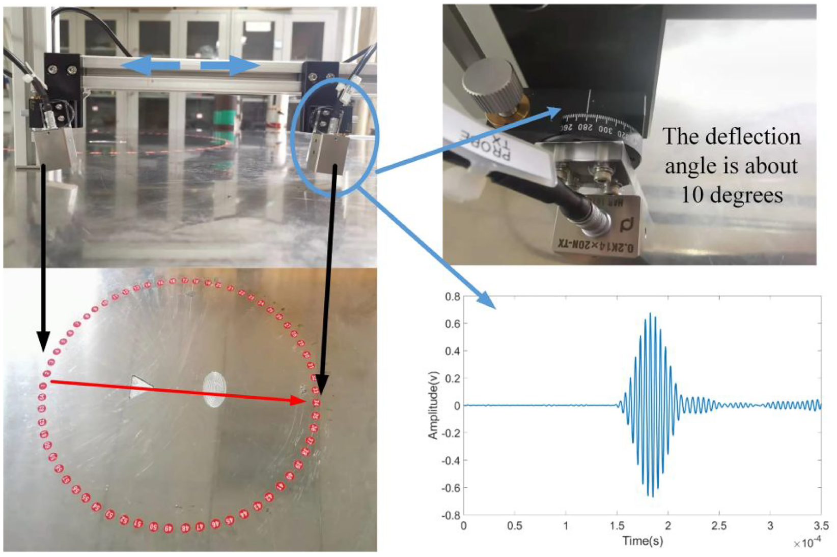
Experimental setup of an air-coupled nondestructive testing system
Reconstruction results
8, 16, 32, and 64 arrays are respectively arranged, and the signals received are treated by the neural network or PCA after FFT, with the imaging results shown in Figure 13. Meanwhile, the thickness distribution across the defect center is extracted and illustrated in Figure 14.
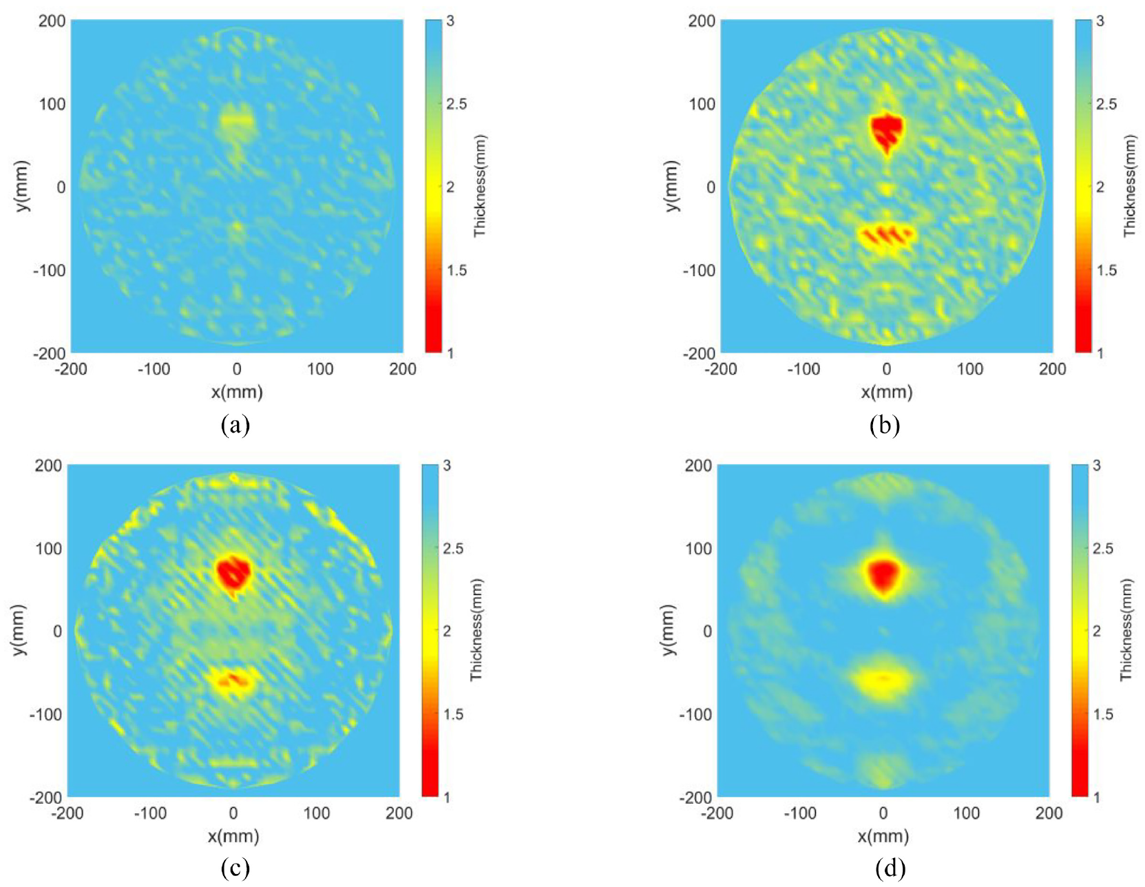
Reconstruction results of triangular and elliptical defects using experimental signals from (a) 8 probes, (b) 16 probes, (c) 32 probes, and (d) 64 probes.
Cross-sections of the thickness reconstructions by experiments. The yellow, green, blue, and black lines represent the results calculated from the 8, 16, 32, and 64 probes, respectively, and the red solid line corresponds to the actual defect.
In summary, sparse arrays, such as 8 or 16 probes, can only identify the defect location. The thickness information is inaccurate. As the probe number increases, the defect profile can be distinguished gradually. For the four cases, the noise pollution of the imaging results is more serious than that in numerical simulations, which may be due to the deviation of the measurement system. In addition, the air-coupled detection system is not limited by the coupling agent. It is difficult to accurately control the exciting point at oblique incidence. In addition, the flat probe has a finite surface area for wave excitation and reception, which also can bring in discrepancies with simulation conditions. Despite those, the results based on experimental signals match well with the numerical simulations. Similarly, RNL can be obtained and shown in Figure 15, which also demonstrates that the thickness distribution in experiments is slightly worse than that of simulations. The depth error from the 64-array imaging is less than 0.25 mm, which efficiently validates the algorithm’s effectiveness once again.
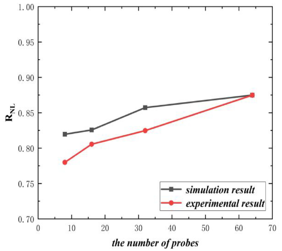
The variation trend of RNL in experiments
Final remarks
The experimental results demonstrate that the algorithm is effective to obtain the thickness imaging for plate-like structures in different arrays. Although the diffraction tomography based on the Born approximation can also reconstruct defects, 20 it still has limitations. The defect must be relative to the wavelength λ and of low contrast relative to the background. Therefore, a lower frequency is usually selected when detecting large flaws.20,21 Accompanying that, the received signal of guided waves at low frequencies is commonly noisier and the imaging resolution will be reduced. Unlike diffraction tomography, the DBIM method adopted in this algorithm overcomes this drawback as the objective function is modified at each iteration step for better convergence.
The iterative approach, widely utilized in full waveform inversion for seismic waves, 22 can also be adapted to reconstruct corrosion-type defects in plates. It usually requires 20–40 iterations, which takes 4.5 h. 22 With the same 64-array conditions set in that case, only 8 iterations are needed in this paper, and each iteration takes less than 3 min when using a common computer with 11th Gen Intel Core i7-11700 @ 2.50 GHz. The Green’s function is recalculated at each step when the objective function is obtained, so that the new scattering features are properly expressed, which induces faster convergence. Additionally, the PCA algorithm decreases the matrix dimensionality, which further improves the computing efficiency.
The rule
Conclusion
In summary, two algorithms that can be suitable for any number of probes are developed and utilized for the reconstruction of various defects. The influence of probe number is systematically investigated from perspectives of simulation and experiments, with the main conclusions drawn as follows:
(1) The MOM has the ability to transform the nonlinear Lippmann-Schwinger equation into a linear form, and the corresponding relationship between the objective function and the thickness is directly established.
(2) Two algorithms of machine learning, that is, neural network and PCA, are developed, both of which have high calculation accuracy when solving the underdetermined and overdetermined equations, respectively.
(3) The defect location can be roughly distinguished if the array is sparse. More probes are needed for reconstructing the specific shape and thickness, especially when multiple defects are included.
The research conducted in this paper is based on a single-mode guided wave. For improving the imaging resolution, a relatively short wave with the central frequency of 200 kHz is utilized. Meanwhile, in order to eliminate the interference of S0 mode, an air-coupled system is designed, which is used for wave generation and reception. A laser vibrometer may be better for improving imaging quality if experimental conditions permit, which is worthy of exploration in the future.
Footnotes
Declaration of conflicting interests
The author(s) declared no potential conflicts of interest with respect to the research, authorship, and/or publication of this article.
Funding
The author(s) disclosed receipt of the following financial support for the research, authorship, and/or publication of this article: The authors gratefully acknowledge the supports of the Natural Science Foundation of China (12061131013, 12172171, and 11972276), the Opening Project of Applied Mechanics and Structure Safety Key Laboratory of Sichuan Province (SZDKF-202002), the State Key Laboratory of Mechanics and Control of Mechanical Structures at NUAA (No. MCMS-I-0522G01), National Natural Science Foundation of Jiangsu Province (BK20211176), Jiangsu High-Level Innovative and Entrepreneurial Talents Introduction Plan (Shuangchuang Doctor Program, JSSCBS20210166), the Fundamental Research Funds for the Central Universities (NS2022011 and NE2020002), Local Science and Technology Development Fund Projects Guided by the Central Government (2021Szvup061), and a project Funded by the Priority Academic Program Development of Jiangsu Higher Education Institutions (PAPD). Prof. Iren Kuznetsova thanks the Russian Ministry of Science and Higher Education (government task #FFWZ-2022-0002) for partial financial supports.