Sage Journals: Discover world-class research

Abstract

Fatigue is a leading cause of structural failure; however, monitoring and prediction of damage accumulation remains an open problem, particularly in complex environments where maintaining sensing equipment is challenging. As a result, there is a growing interest in virtual loads monitoring, or inferential sensing, particularly for predicting strain in areas of interest using machine learning methods. This paper pursues a probabilistic approach, relying on a Gaussian process (GP) regression, to produce both strain predictions and a predictive distribution of the accumulated fatigue damage in a given time period. Here, the fatigue distribution is achieved via propagation of successive draws from the posterior GP through a rainflow count. The establishment of such a distribution crucially accounts for uncertainty in the predictive model and will form a valuable element in any probabilistic risk assessment. For demonstration of the method, distributions for predicted fatigue damage in an aircraft wing are produced across 84 flights. The distributions provide a robust measure of predicted damage accumulation and model uncertainty.

Keywords

Gaussian process probabilistic fatigue assessment posterior sampling uncertainty propagation data-driven strain prediction

Introduction

Structures are frequently retired with a large remaining useful life due to fatigue damage present before cracks are detectable. To assess this level of damage, a knowledge of the loading history of the structure is required. One provision for this could come from installed strain gauges; however, for large structures, and/or structures operating in harsh environments such as aircraft or wind turbines, maintaining such a sensor network is currently infeasible. Alternatively, budgetary constraints may mean that sensing equipment is not installed at the commissioning stage or is only available for a limited monitoring period. As a result, there is a growing interest within the structural health monitoring community in predicting loading histories indirectly. This is often referred to as virtual loads monitoring^1,2 and, ideally, would be possible to do from routinely available measurements.³ Where accurate prediction proves possible, one may use the predicted loads to characterise and refine the loading spectrum that the structure is assumed to withstand and gain a greater understanding of the level of damage that the structure has withstood. This enables both a reduced cost of ownership, due to the reduced requirement for inspection and conservative replacement, and a reduced risk of failure due to the enhanced ability to identify otherwise unforeseen structural problems.

Fatigue analysis can be broken down into three broad types: stress-life (S-N), strain-life ( $ϵ - N$ ) and a linear elastic fracture mechanics approach.^4,5 This work will focus on stress-life fatigue analysis, suitable for problems where there may be zero crack tolerance (such as aircraft landing gear which follows a safe-life design practice) or where physical inspections may be difficult (such as offshore wind turbines). This approach relies upon material S-N curves, describing how many cycles a material can withstand at a given stress range before failure. Large safety factors are frequently used in S-N fatigue analysis due to uncertainties related to load estimates and stress calculation, fatigue strength models or the natural randomness of fatigue material properties.⁶

To predict fatigue damage, a knowledge of loads across the structure at areas of interest is required. Two varying approaches in the literature consider either a physics-based or data-driven modelling approach. From the physics-based view point, finite element model updating has been considered by a number of researchers in situations where limited data are available. This has been achieved using vehicle weigh-in-motion data for conducting fatigue assessment on road bridges.^7,8 Based on the damage equivalent load (DEL) concept, Ziegler et al.⁹ use limited data in combination with aero-hydro-elastic simulations to update finite element models for extrapolation of fatigue damage prediction to locations across a monopole wind turbine where measured data are not available.

An alternative to physics-based modelling approaches is to utilise data-driven methods, which are increasing in popularity. Ziegler et al.¹⁰ present a methodology for wind turbines that opts for a regression based prediction when measured data are available at the location of interest as an alternative to the updated finite element model approach discussed previously. Avendano-Valencia et al.¹¹ use Gaussian process (GP) regression to provide a probabilistic fatigue estimate also based on the DEL concept, predicting the equivalent load using readily available data such as wind speed and turbulence intensity. Virtual loads monitoring of aircraft have used global parameters such airspeed and local measurements of, for example, acceleration to build regression models for predicting loads elsewhere. Machine learning methods have been used to predict strain on landing gear³ and at points across the main body of aircraft.^1,12 Such methods have also been extended to fatigue life assessment indirectly, using the strain prediction in S-N fatigue analysis.^1,12 Azzam et al.¹³ use the so-called indirect fatigue prediction model, importing some physical knowledge of helicopter rotor blades to train an artificial neural network to predict fatigue damage without predicting strain as an intermediate step.

Aim and contribution

A level of uncertainty in fatigue damage assessment is unavoidable. However, by pursuing a probabilistic assessment, we can allow and account for uncertainty in a controlled manner. Even in the situation where full strain measurements are available in the areas of concern, uncertainty is still present due to sensor noise. Pursuing a predictive strain model in the absence of measurements can only increase this uncertainty, which, in our view, necessitates a probabilistic approach. To fully utilise a probabilistic strain prediction, the resulting fatigue damage assessment should also be treated probabilistically. Doing so enables a greater value to be acquired from the assessment – rather than relying on large factors of safety to account for uncertainty, we can assess risk in a more controlled and evidence-based manner. How this information could be used varies depending on the application. For safe-life applications, for example, a risk-based methodology could be adopted to inform maintenance schedules and perhaps enable a greater service life to be achieved for components or structures.

A number of the studies cited above have employed GP regression.^3,12 As a Bayesian method, the output of the GP is a posterior distribution. While the usefulness of GP regression for strain prediction has been shown previously, the inherent probabilistic nature of the model is frequently ignored – often only the mean prediction is used within the literature. Many modelling approaches show the prediction of strain but stop short of propagating these predictions into a fatigue accumulation estimate, where they have done, the estimates of fatigue damage presented in the literature are solely a deterministic prediction using the GP posterior mean.^12,14 To provide a probabilistic assessment of fatigue accrual here, we will take advantage of the entire posterior distribution of the GP to characterise the uncertainty of our load prediction and assess the impact that this has on fatigue damage.

Rather than providing a single deterministic prediction of strain at a given time point, a GP provides a distribution of possible strain values. Furthermore, any finite number of these will be jointly Gaussian, allowing one to draw samples of the possible strain time histories (i.e. those that are likely given evidence from data) from the process. Here, the approach suggested is to take a large number of draws from an established GP and feed each one through a rainflow counting algorithm to establish a distribution of predicted fatigue damage. Due to the ‘black-box’ nature of the fatigue assessment procedure, in particular the rainflow counting method, such a distribution of fatigue cannot be calculated analytically. Thus, such Monte Carlo methods are required to develop understanding of the damage distribution.

Treating fatigue as a probabilistic problem is considered to be one of the most important ways of reducing our reliance on large factors of safety within fatigue analysis,^15,16 and harnessing the probabilistic potential of predictions is, therefore, crucial. Previous studies have not performed this step and the proposed method here allows us to propagate the uncertainty of the model through the fatigue assessment. It is the authors view that the resulting distribution of damage is the true reflection of the GP model, as opposed to a deterministic assessment typically found, and here we will show that an increased robustness is achieved as a result.

There are two types of uncertainty: aleatoric and epistemic. The former is related to the uncertainty of the result, which in this case could be considered to be the error of the strain gauges that are used to train the model. This type of uncertainty is considered by Reed,¹ where an error of ±5% on the strain gauges is simulated and a subsequent upper and lower limits on the measured fatigue damage are shown. Epistemic uncertainty is related to the uncertainty of the model and is often the result of the availability of data. While epistemic uncertainty can be reduced with the use of increasing data, within a data-driven approach there are conflicting demands. First, the quantity of data is not necessarily the limit, but the availability of training data that is representative of the testing conditions. Second, there are considerable computational demands that need to be considered. For GP regression, the cost of training the model is $O (m^{3})$ while drawing samples from the model requires the inversion of the complete posterior covariance matrix with cost $O (n^{3})$ , where m and n are the number of training and testing points, respectively. This work is looking at uncertainty of both types: the noise hyperparameter represents the uncertainty in the data, while the magnitude of the posterior variance is also a function of the distance between the training data (model inputs) and test data, see Equation (4).

The GP regression framework and suggested approach for fatigue damage distribution estimation are introduced and discussed in more detail in the next section. The approach is then demonstrated using a loads monitoring case study for a Tucano aircraft.^1,14

While an aerospace application is used for the case study within this work, the methodology is valid for many other applications such as offshore, rotating machinery and many other civil and mechanical applications where strain predictions can be used to inform a fatigue assessment. The application and design methodology would influence how the resulting damage distribution is used, that is, for critical structures with a high cost of failure, the most conservative damage sample may be used.

GP regression

GP regression is a powerful machine learning technique, popular within the structural health monitoring field.^17–19 GP regression is a non-parametric method, meaning that it does not specify a defined functional form, but rather a distribution over functions that are coherent with the data that the process is conditioned by. 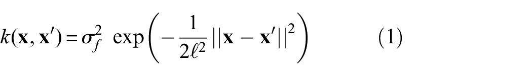A GP is specified by the choice of a mean and a covariance function, $k (x, x')$ , where $x$ and $x'$ are distinct inputs to the GP. A zero mean prior is often assumed and the squared exponential is one of the most commonly used covariance functions²⁰ (also employed here):

k (x, x') = σ_{f}^{2} \exp (- \frac{1}{2 ℓ^{2}} | | x - x' {| |}^{2})

(1)

where $σ_{f}^{2}$ and $ℓ$ are the signal variance and lengthscale hyperparameters, respectively.

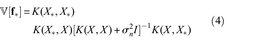
Using Equation (1), predictions now can be specified as a function of $K (X, X)$ , the covariance matrix of the training input values, $K (X_{*}, X)$ , the covariance matrix of the test (prediction) and training input values, $K (X_{*}, X_{*})$ , the covariance matrix of the test input values, and $y$ , the observed training output/target values.

During the training stage, the hyperparameters in Equation (1) are optimised by minimising the negative log marginal likelihood:

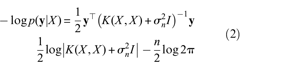
\begin{matrix} - \log p (y | X) = \frac{1}{2} y^{⊤} {(K (X, X) + σ_{n}^{2} I)}^{- 1} y \\ \frac{1}{2} \log | K (X, X) + σ_{n}^{2} I | - \frac{n}{2} \log 2 π \end{matrix}

(2)

where I is the identity matrix and n is the number of training points used. The noise hyperparameter $σ_{n}^{2}$ represents the variance of noise $ϵ$ . This is required as real-world situations are unlikely to follow a function $y = f (x)$ , but rather a noisy representation of this $y = f (x) + ϵ$ . After optimising the hyperparameters, the GP posterior mean, $E [f_{*}]$ , and covariance, $V [f_{*}]$ , functions can now be defined by Equations (3) and (4), respectively²⁰:

E [f_{*}] = K (X_{*}, X) [K (X, X) + σ_{n}^{2} I]^{- 1} y

(3)

\begin{matrix} V [f_{*}] = K (X_{*}, X_{*}) \\ K (X_{*}, X) [K (X, X) + σ_{n}^{2} I]^{- 1} K (X, X_{*}) \end{matrix}

(4)

Sampling from the GP

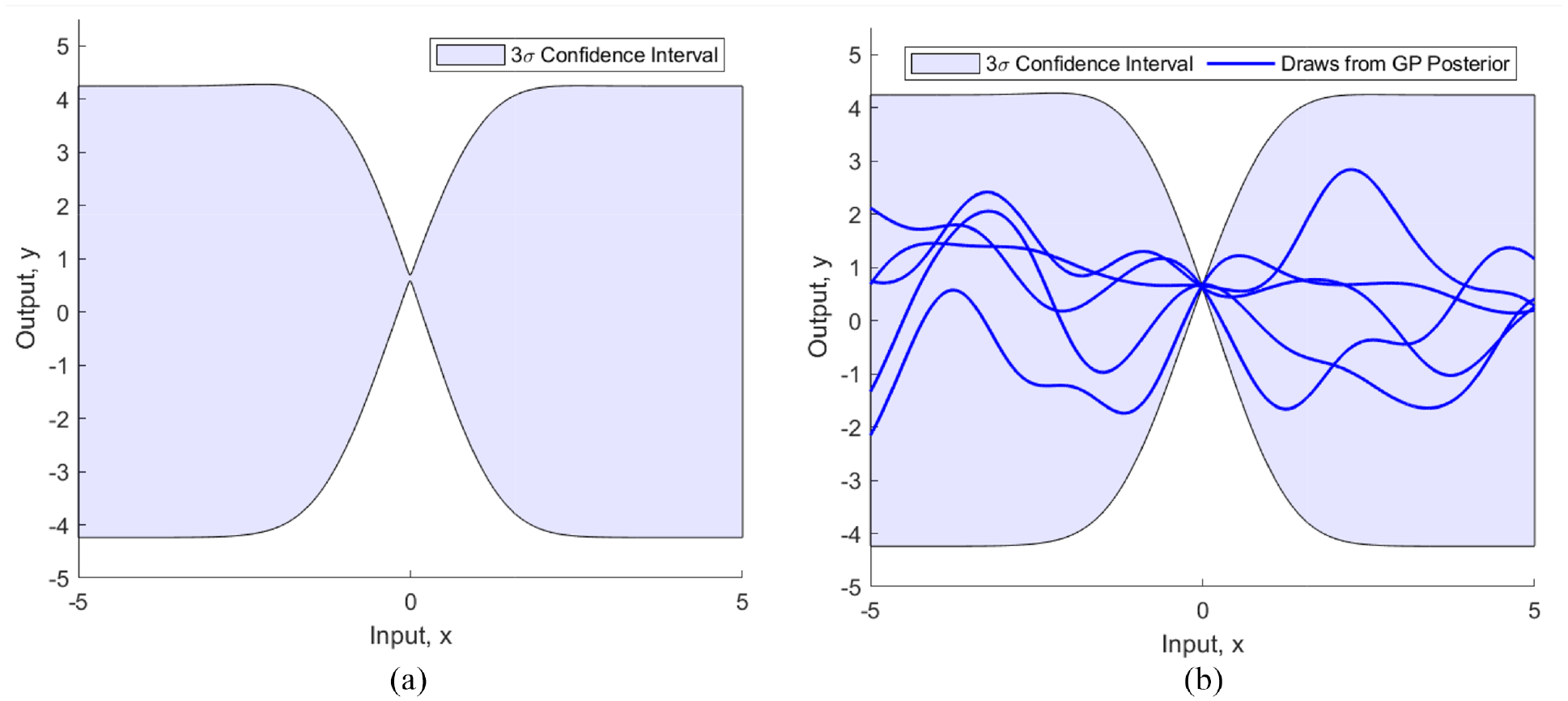
A feature of GP regression is that the distribution of any finite number of points in the output space is jointly Gaussian. This results in an infinite number of functions that can fit, or be drawn from, the posterior distribution. Figure 1(a) illustrates an arbitrary GP posterior distribution that has been conditioned on a single data point at $x = 0$ , while Figure 1(b) shows a series of functions that this non-parametric model can fit, which are often referred to as ‘draws’ from the posterior distribution. Each function fits to the training/conditioning point, away from the training data the behaviour of the functions are characterised by the prior covariance function.

Figure 1.

(a) $3 σ$ confidence intervals of (generic) Gaussian posterior, and (b) functions drawn from the posterior distribution.

The proposed method involves sampling from the posterior distribution of the GP model trained to predict strain at a given location. The novel concept in this work arises from the notion that there is no specific $f (x)$ that characterises the data, but infinite $f (x_{i})$ instead. By calling upon a large number of these functions, a probabilistic prediction for fatigue can be built from the GP posterior distribution. Specifically, by generating a large number of draws from the posterior and using the stress-life fatigue methodology to assess damage, we will be able to generate a distribution for damage accumulation given a GP strain prediction.

Samples/draws are generated from the posterior by calculating (²⁰):

f_{sample} = E [f_{*}] + L u

(5)

where $E [f_{*}]$ is the GP mean prediction calculated using Equation (3), $u$ follows an independent Gaussian distribution, $u ~ N (0, I)$ . $L$ is the lower triangular matrix of the Cholesky decomposition of the posterior covariance, such that $V [f_{*}] = L L^{T}$ , where $V [f_{*}]$ is the posterior covariance, Equation (4). This process is used to generate the draws in Figure 1.

It should be noted that this process is not equivalent to generating samples by adding the mean prediction, $E [f_{*}]$ , to Gaussian noise scaled over the magnitude of the confidence interval. Such an approach would have sampled values independent from each other and would result in effectively generating small fatigue cycles within the confidence interval, as shown in Figure 2.

Figure 2.

Sample taken from GP posterior compared to an independently sampled noise process.

Assessing the model

The normalised mean squared error (NMSE), defined by Equation (6), is frequently used as a metric of assessing the prediction accuracy and will also be employed here.

NMSE = \frac{100}{n σ_{y}^{2}} \sum (y_{p} - y_{i})^{2}

(6)

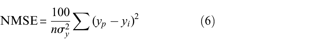
where $y_{p}$ and $y_{i}$ are the values of the prediction and the measured data at data point i, $σ_{y}$ is the standard deviation of the measured values and n is the number of data points.

Cycle counting for fatigue analysis

Following the sampling process described above, the strain predictions are converted into an equivalent stress. For fatigue analysis, this must then be converted into a set of stress ranges and mean stresses. This is achieved here using the rainflow cycle counting process following the ASTME 1049 standard.²¹

Calculating fatigue damage

Following the rainflow cycle count, the damage for each sample can be calculated using Miner’s rule:

D = \sum \frac{n_{i}}{N_{i}}

(7)

where $n_{i}$ and $N_{i}$ are the number of cycles in the stress response at a given stress range (taken from the rainflow cycle count) and the number of cycles to failure the material is capable of withstanding at that stress level, respectively. The latter value can be found from material S-N curves, which are found empirically. $D$ is the summation of damage from each of the individual stress cycles identified within the stress response, with the material expected to fail when $D = 1$ . Therefore, ‘damage’ within the context of this work will be the estimated proportion of the materials fatigue life that has been used within a flight.

The flowchart in Figure 3 outlines the process

Figure 3.

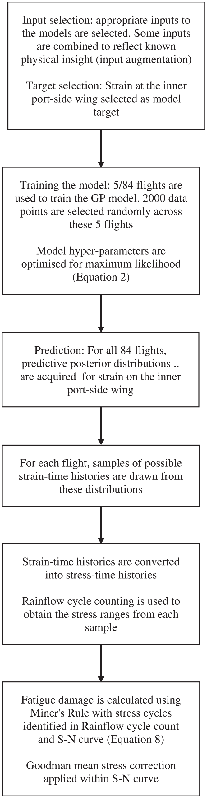
Flowchart of proposed methodology.

Case study: Tucano aircraft

To demonstrate this methodology, a case study is used from a loads monitoring campaign of a Tucano short aircraft.¹⁴ Data are available from strain measurements across the aircraft for a range of flights, and the measured strain at the inner port-side wing shall be used as the target variable. Candidate inputs to the GP model are standard in-service measurements, such as acceleration measurements on the plane wings and at the centre of gravity, airspeed and altitude. Following Reed,¹⁴ minor semi-physical adjustments²² were made to some of the inputs prior to use within the model: the indicated airspeed was squared to give an indication of dynamic pressure and the acceleration measurements used were multiplied by the mass of the aircraft to give an indication of forces at the respective locations.

At a downsampled rate of 16 Hz, each of the flights has between 20,000 and 90,000 data points. The GP posterior sampling operation requires a matrix inversion of complexity $O (n^{3})$ and therefore, for computational reasons, the study here is limited to 10,000 data points from each flight for the purpose of demonstration. The most damaging 10,000 data points in each flight are selected (based on fatigue analysis performed on the measured data prior to prediction) to ensure that non-negligible damage accumulation occurs in the studied time history. The downsampling of data to 16 Hz does result in some loss of dynamic strain behaviour for some of the flights. However, the available inputs to the model are only available at 16 Hz and, therefore, this work shall only be assessing the quasi-static behaviour shown at this sampling frequency.

Fatigue analysis is performed using the S-N curve described by Reed for an L-65 aluminium alloy, including the Goodman mean stress correction¹⁴:

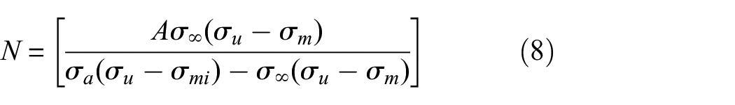
N = [\frac{A σ_{\infty} (σ_{u} - σ_{m})}{σ_{a} (σ_{u} - σ_{mi}) - σ_{\infty} (σ_{u} - σ_{m})}]

(8)

where N is the number of cycles to failure at a given stress range, $σ_{u}$ is the ultimate tensile strength of the material, $σ_{m}$ and $σ_{mi}$ are the cycle mean stress and S-N curve mean stress, respectively. The numerical constant A can be found in Reed.¹⁴ The GP regression model was trained using 2000 data points, randomly selected from five training flights and then tested on all 84 flights (including the five training flights). Note that none of the flights presented below (i.e. flights 1, 2 and 3) were within the training set. For each flight prediction, 10,000 draws are taken from the GP posterior and fed through the fatigue assessment to create a distribution of predicted fatigue damage accrual for each flight. This is compared to the equivalent damage arising from the measured strain data as a benchmark.

The strain prediction shows a very good level of accuracy across the flights, with 82 of the 84 flights having a NMSE value less than 15.7% with the majority of these being below 5%. The range of errors are displayed in a histogram shown in Figure 4. There are two flights with NMSE values greater than this (31.1% and 46.9%). These two flights showed very low stress amplitudes (leading to very little accumulation of damage) which are difficult to capture due to their benign nature and this amplifies the modelling error. The measured data are captured within the confidence intervals for both of these predictions.

Figure 4.

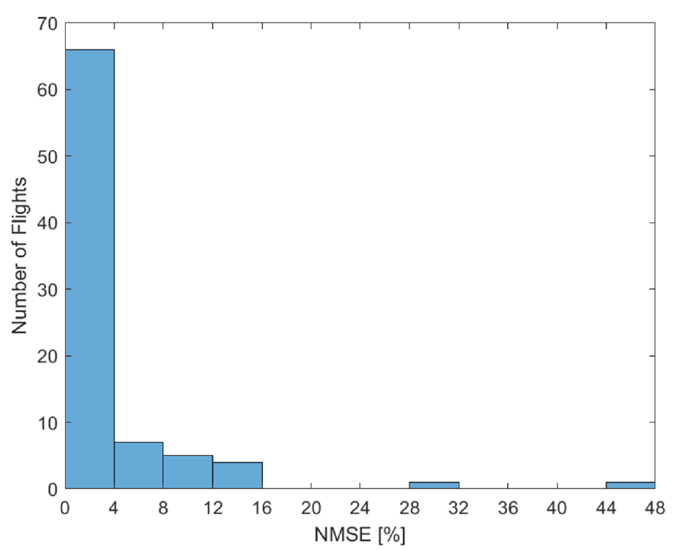
Histogram of NMSE values for the 84 flights.

Here we will first show the results from an exemplar flight to present the methodology, before considering predictions for all 84 flights and discussing the fatigue damage results for two outlying flights in further detail. The accuracy of the strain prediction arising from the GP posterior mean prediction for this exemplar flight was very good, equalling 1.4% and making the prediction one of the most accurate in the test set; however, the flight itself is one of the more damaging in terms of fatigue accrual and is therefore interesting to study as the first example.

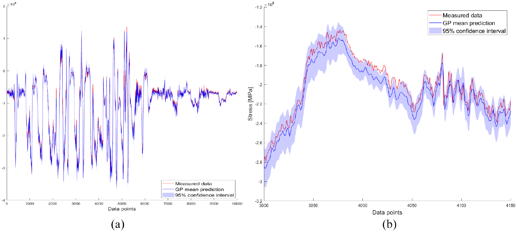
The GP prediction and posterior draws for the example flight can be seen in Figure 5. From this, one can see that the prediction is very good: the measured value is within the confidence interval across the flight and, crucially, at the extreme maxima and minima, the prediction matches the measured data well. An enhanced view of this flight can be seen in Figure 5(b), which also displays 15 of the 10,000 samples taken from the posterior distribution. We can see that in the areas of flight where there are low stress fluctuations, the samples appear as a mean offset from the GP mean prediction. This is desirable, as the model is capturing the underlying physics of the region well, but with some level of uncertainty about the magnitude of the stress.

Figure 5.

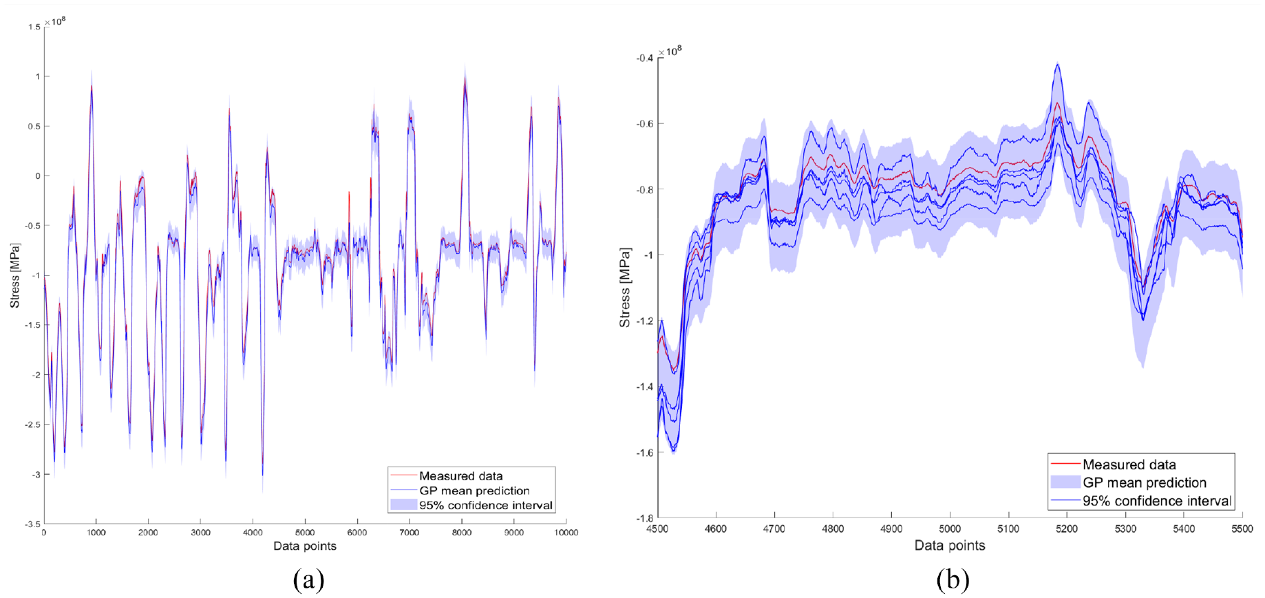
Example flight (flight 1): (a) posterior GP, and (b) enhanced view of (a) with posterior draws shown.

The output of the fatigue assessment for each of the GP posterior samples provides a distribution of damage for each flight. The histogram shown in Figure 6 presents this distribution for flight 1. Also shown are the damage accumulation values when the GP mean prediction and the measured data themselves are fed through the rainflow counting algorithm. We can see that while the GP mean and measured fatigue assessments agree closely, the mean of the sampled damages is more conservative. We can see that the mode average of the sampled damages (i.e. the most likely value in the histogram) performs better than the mean at predicting the measured damage state. The conservative result of the mean of the sampled damages is to be expected due to the non-linear relationship between stress cycle range and fatigue damage (see Equation (8)), where larger ranges cause more damage. By sampling from the GP posterior, on a cycle-by-cycle basis, we would expect to see a distribution of stress cycle ranges either side of the mean prediction value. The impact of these larger cycles would, therefore, result in a more conservative damage prediction from the mean of the samples compared to the posterior mean prediction.

Figure 6.

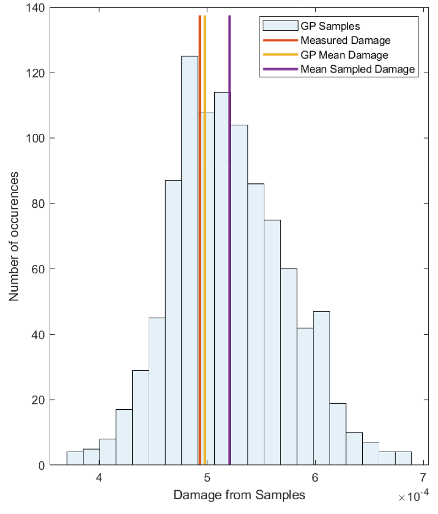
Histogram of damages for flight 1.

The predicted fatigue accumulation distributions for all 84 flights are visualised in Figure 7(a). Each vertical contour shown represents the damage distribution for a single flight and the solid line marks where the predicted damage is equal to the damage accrual from the measured strain data. One can see that for each flight the predicted damage distributions encompass the ‘measured’ damage. Circular markers are added to show the fatigue damage prediction when the GP mean is used.

Figure 7.

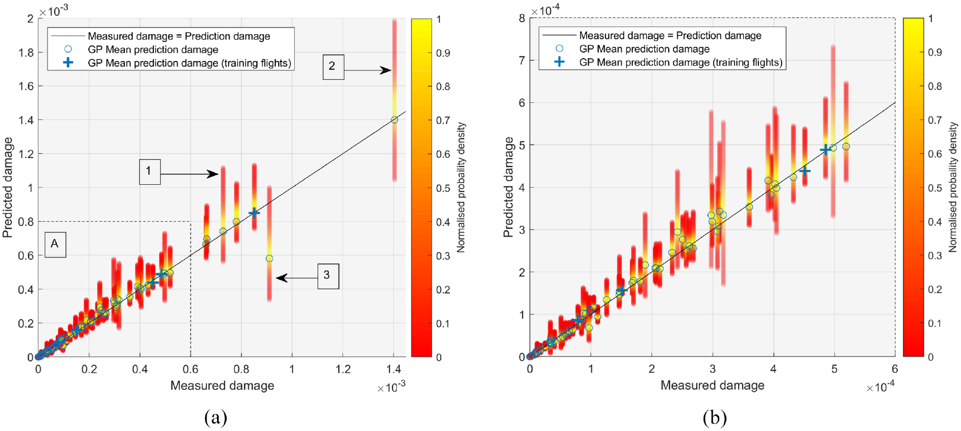
Fatigue damage distributions from the GP Mean, individual posterior samples and measured data. The GP mean prediction for the training flights is indicated with a ‘+’ symbol: (a) all 84 flights and (b) region A of (a).

The majority of flights occur in region A, a zoomed view of which is provided in Figure 7(b). The overall trend shown is that the most likely value from the sampled damages is more conservative than the mean GP prediction which, as discussed, is an expected result of sampling and attributing more damage to larger cycles. We can also see that the variance of the damage distribution generally increases with an increase in flight damage. There are two main factors that impact this – cycle stress range and cycle mean stress.

To explain this, Figure 8 shows how the variance of damage grows with increased variance in cycle amplitude and mean. The blue line shows the relationship between cycle amplitude/range and damage (see Equation (8)). The uncertainty associated with cycle amplitude is shown in purple (here the cycle range is sampled from a Gaussian distribution with a standard deviation equal to 2% of the stress amplitude). The effect of having an uncertainty on the mean stress of ±100 MPa is shown in pink, where one can see the significant growth in damage variance. Sampling from the posterior distribution can lead to large changes in the mean stress of the largest (and most damaging) cycles. The impact that this can have over thousands of stress cycles is large, and difficult to fully understand or predict due to the ‘black box’ nature of the rainflow cycle counting process. For both sources of uncertainty, we can see that the impact of uncertainty is nonlinear, with the impact of increased damage being greater than a reduced damage, as is borne out the predictions shown in Figure 7(a) and (b).

Figure 8.

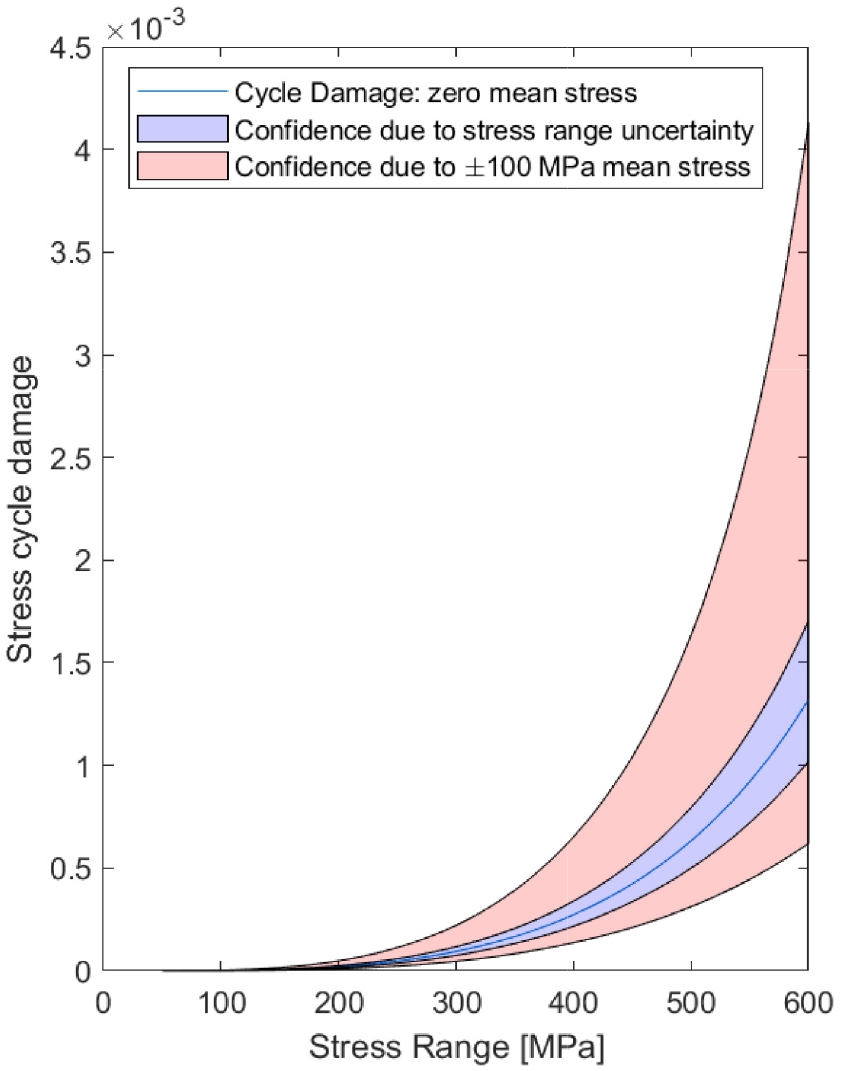
Impact of cycle mean stress and uncertainty of stress cycle range on damage.

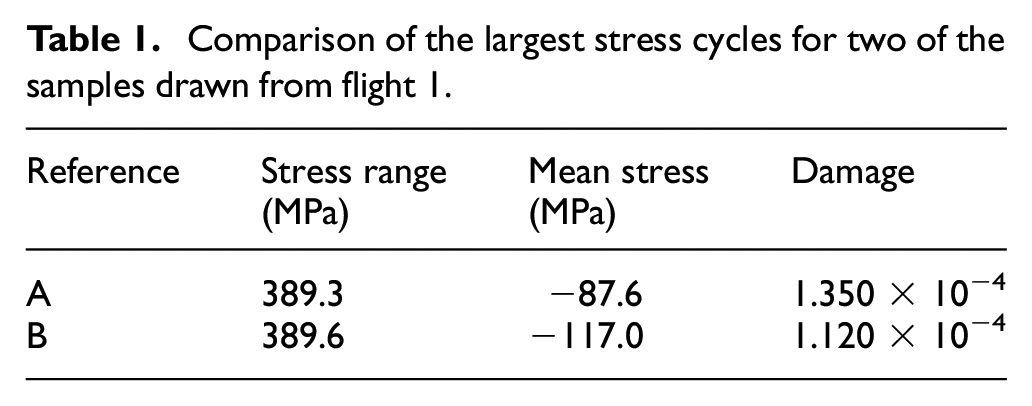
In Table 1, we can see the details of the largest stress cycles of two of the draws from the GP for flight 1. Despite the stress ranges for the two cycles being almost equal, we can see that cycle B is around 19% more damaging than cycle A, as a result of the difference in mean stress. When a large amount of the damage for each flight arises from a small number of large stress cycles (see Figures 10 and 12), the impact of this of the damage on the sampled flight is significant.

Table 1.

Comparison of the largest stress cycles for two of the samples drawn from flight 1.

Reference	Stress range (MPa)	Mean stress (MPa)	Damage
A	389.3	−87.6	1.350 × 10⁻⁴
B	389.6	−117.0	1.120 × 10⁻⁴

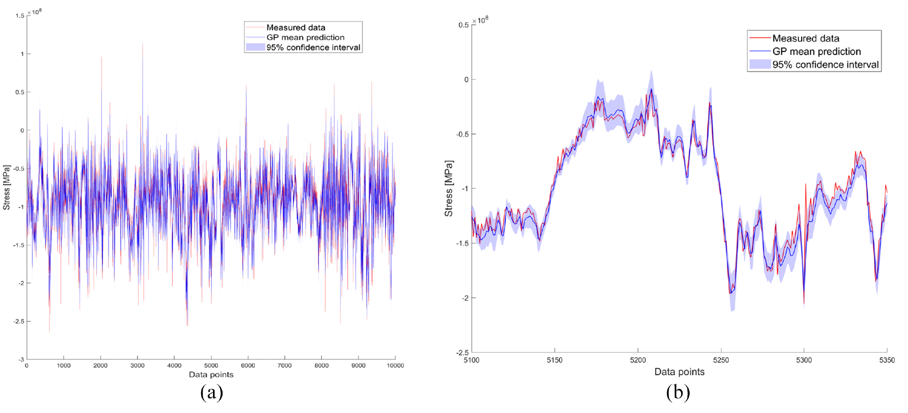
We will now look at two flights, identified as flights 2 and 3 in Figure 7(a). Flight 2 is the most damaging flight of the test set. Figure 9(a) shows the predicted versus measured stress for this flight, with an enhanced section shown in Figure 9(b) where it can be seen that the model performs well across a varied stress response. The NMSE for the GP mean prediction is 0.9%. We can see that there is a small mean offset when comparing the mean prediction to the measured data, but for the majority of the flight, the measured value is captured within the confidence bounds of the prediction and crucially, the important characteristics of the stress response are captured, with the turning points shown in the measured data are reflected in the prediction. This translates to a low error in both the damage estimate from the GP mean and the mean of the estimated damage distribution (0.4% and 5.5%, respectively).

Figure 9.

Flight 2: GP posterior and enhanced view: (a) Posterior GP stress prediction and (b) enhanced view of (a).

As discussed above, one can also note the increased variance in the estimated distribution at this level of damage. The load spectra (stress ranges vs cycle counts) from the measured strain and from the most and least damaging samples drawn from the GP are shown in Figure 10. The plot also shows the progression of damage across the stress distribution for the measured data and, as discussed, we can see that the majority of damage is caused by a relatively small number of high stress cycles. As the variance of damage is greatest at high stress levels (Figure 8), we would expect to see an increase in the stress ranges demonstrated by the most damaging sample. Indeed, this can be seen in Figure 10 alongside a reduction in the maximum stress range seen by the least damaging sample for this flight.

Figure 10.

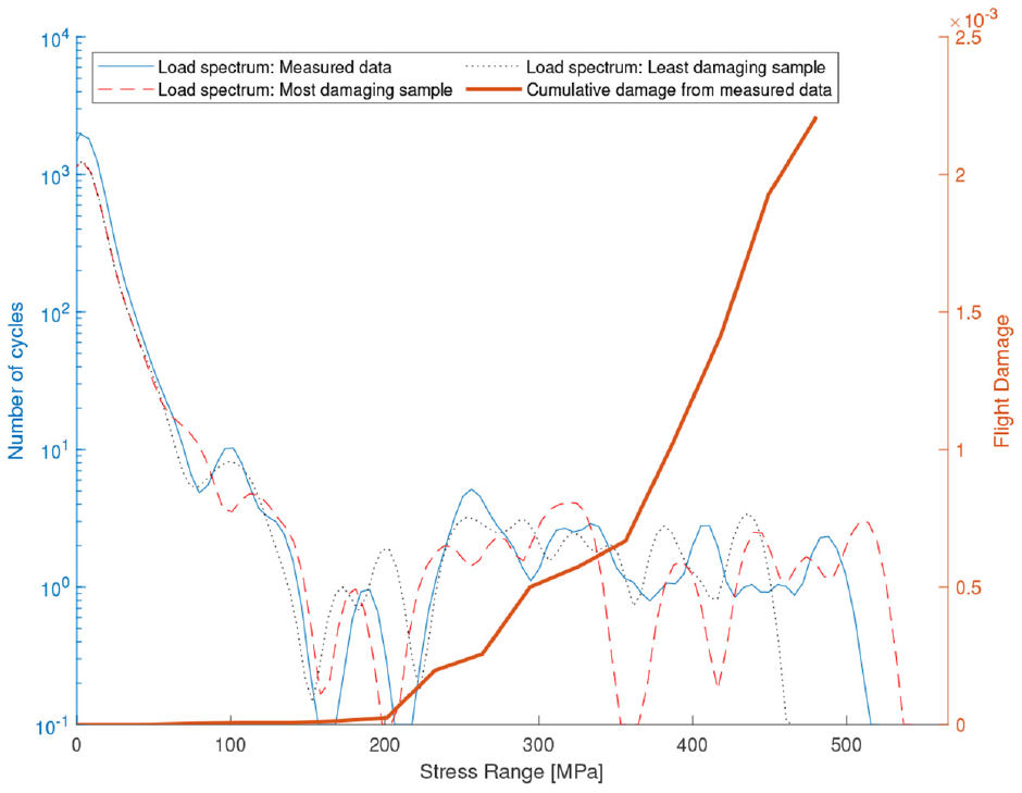
Load spectrum for flight 2.

As discussed, flight 3 has the largest error of the 84 test flights in terms of fatigue damage prediction accuracy, with the GP mean prediction underestimating the measured damage by 44.2%. The GP posterior for this flight can be seen in Figure 11(a) and (b). The mean of the sampled damages is able to reduce this error to 36%. Despite this, the NMSE for flight 3 is only 9.8% (there are numerous flights with greater errors; see Figure 4). We can see, therefore, that NMSE is not necessarily a good indicator of whether a model will be able to predict fatigue damage accrual well, as it is the accuracy of at the local maxima and minima of the largest stress cycles that is most important here, which is not reflected in an error metric which looks at the average error across the stress response. The predicted damage distribution, however, does encapsulate the measured accrual and would allow for a structural health assessment to account for that level of damage at the given probability. The low probability assigned to this level of damage can be explained by the load spectra for this flight (Figure 12), where it can be seen that both the most and least damaging samples underestimate the magnitude of the largest stress ranges.

Figure 11.

Flight 3: GP posterior and enhanced view: (a) Posterior GP stress prediction and (b) enhanced view of (a).

Figure 12.

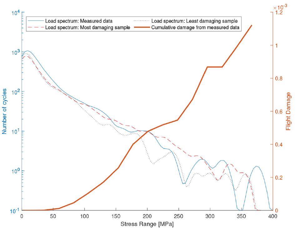
Load spectrum for flight 3.

Discussion and conclusions

The proposed methodology provides a probabilistic prediction of strain and fatigue accrual at unmeasured locations on a structure under an unknown loading. We have shown here that the GP regression model was able to accurately predict strain across the flights, with 98% of flights having a NMSE of less than 16% (Figure 4). The resulting distributions of fatigue are able to shed light on the range of potential damage accrued, with the measured damage state captured within the distribution across all of the flights.

The central argument of this work is that predicting fatigue accumulation indirectly using GP regression as a virtual strain sensor should be considered as a distribution rather than deterministic value. Using only the posterior mean to predict fatigue damage, one of the benefits of using GP regression – its inherent probabilistic nature – is lost. Indeed, it could be argued that a single, deterministic, value for fatigue damage is not truly representative of the posterior distribution of the model. We can see from Figure 7(a) and (b) that the probability of detection of the measured damage state for some flights is low. The results from flight 3 (Figure 11) provide an excellent of example of the usefulness of the approach taken here. While the applied usage of the damage distribution would depend on the individual structure and the potential cost of failure, if one were employing a deterministic strain prediction for this particular flight, or if one were simply relying on the GP mean, the predicted fatigue would be very misleading. The predicted fatigue distribution from the propagation approach, however, incorporates the true damage accumulated (albeit at a low probability). Any following risk assessment employing the distribution would be much more robust to the error in the (mean) prediction of the strain. Regardless of modelling choices, kernel selection and hyperparameter optimisation, in a data-driven environment, accurately predicting the damage using the mean prediction would be unlikely for all scenarios. Therefore, utilising the proposed methodology of sampling to develop damage distributions provides a more robust framework that can be utilised differently based on the nature of the structure. Future work will discuss ways of improving model accuracy for both the GP mean and samples drawn from the posterior. Furthermore, future work will aim to extrapolate the proposed methodology to locations on structures where measured data are not available for training.

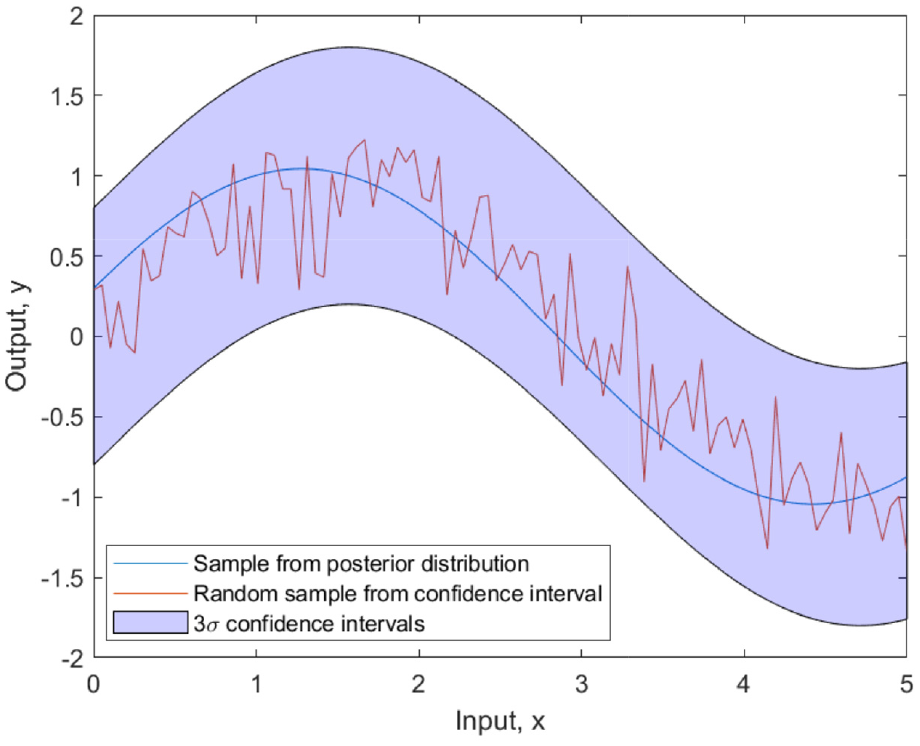
One can extract key features of interest from the predicted fatigue distributions. For example, the method provides a principled means of extracting the least and most damaging strain time histories possible for a given flight that may be used to inform a (e.g. interval based) risk assessment. An alternative means of predicting, for example, the most damaging strain time history possible for a given flight could be to sample a function that passes through the maxima/minima of the posterior GP mean plus/minus the confidence interval. An example of such a function $\pm 2 σ$ is shown in Figure A1 in the appendix. Such a naive approach neglects the joint Gaussian assumption the model is based on and produces a fatigue prediction that is a 350% over-prediction of the measured value.

While the authors advocate exploiting the probabilistic nature of the GP model, or any probabilistic model, care must be taken in how uncertainty assessments are interpreted. The uncertainty in the GP prediction is based on a measure of the distance between input training and testing points. The inputs to the GP are specified by the user and the distance measure dictated by the covariance function. This means that the predictive distributions of fatigue shown here are dependent on the selection of both of these things. So long as the strain prediction quality is acceptable, the selection of the covariance function should not be of large consequence. However, care must be taken in selection of the model inputs. For example, if an irrelevant input were included which exhibited different behaviour between training and testing sets, this would increase the uncertainty on the fatigue damage assessment in an unrepresentative manner. Here we advocate the use of an Automatic Relevance Determination (ARD) covariance function²³ with a separate lengthscale for each input to mitigate the effect of a potentially mis-specified input variable. Finally, it is important to note that, as with all data-driven methods, prediction quality and reliability of the confidence bounds will decrease in extrapolation. If the relationships between inputs and targets change outside of the training dataset, the inference here will not be valid. The importance of a representative training set cannot be understated.

In this work, uncertainty in strain prediction is quantified through the GP framework and propagated through to the final fatigue assessment. It should be recognised that in all forms of model (data driven, finite element analysis), understanding the uncertainty within the result is desirable. Here, the method accounts for the uncertainty from measurement noise and model predictions. By propagating this uncertainty, we can achieve an improved reliance upon the model predictions.

One crucial question is therefore, how to actually use the resulting distribution. Ultimately, a structure’s usage will dictate this and a risk-based maintenance and inspection strategy can be formed accordingly.²⁴ The original design methodology of the structure, that is, Safe-Life or Fail-Safe, will influence this, alongside other factors including the level of uncertainty of the prediction.

Footnotes

Appendix

Acknowledgements

The authors would like to thank Steve Reed from the Defence Science and Technology Laboratory (DSTL) for the data that has enabled this study.

Declaration of conflicting interests

The authors declared no potential conflicts of interest with respect to the research, authorship and/or publication of this article.

Funding

The authors disclosed receipt of the following financial support for the research, authorship and/or publication of this article: This work was supported by the Engineering and Physical Sciences Research Council [grant number EP/S001565/1].

ORCID iD

Samuel J. Gibson

References

Reed

SC.

Development of a parametric-based indirect aircraft structural usage monitoring system using artiﬁcial neural networks. Aeronaut J 2007; 111(1118): 209–230.

Robertson

IN.

Prediction of vertical deﬂections for a long-span prestressed concrete bridge structure. Eng Struct 2005; 27(12 SPEC. ISS.): 1820–1827.

Holmes

Sartor

Reed

, et al. Prediction of landing gear loads using machine learning techniques. Struct Health Monit 2016; 15(5): 568–582.

Pan

Lin

SH.

Fracture mechanics and fatigue crack propagation. In: Lee

Pan

Hathaway

Barkey

(eds.) Fatigue Testing and Analysis, chapter 6. Burlington, MA: Butterworth Heinemann, 2005, pp.237–284.

McDowell

DL.

Basic issues in the mechanics of high cycle metal fatigue. Int J Fract 1996; 80(2): 103–145.

Halfpenny

Chabod

Czapski

, et al. Probabilistic fatigue and reliability simulation. Procedia Struct Integr 2019; 19: 150–167.

Hajializadeh

OBrien

O’Connor

AJ.

Virtual structural health monitoring and remaining life prediction of steel bridges. Can J Civ Eng 2017; 44(4): 264–273.

Guo

Frangopol

Chen

Fatigue reliability assessment of steel bridge details integrating weigh-in-motion data and probabilistic ﬁnite element analysis. Comput Struct 2012; 112–113: 245–257.

Ziegler

Smolka

Cosack

, et al. Brief communication: structural monitoring for lifetime extension of offshore wind monopiles: can strain measurements at one level tell us everything? Wind Energy Sci 2017; 2(2): 469–476.

10.

Ziegler

Cosack

Kolios

, et al. Structural monitoring for lifetime extension of offshore wind monopiles: veriﬁcation of strain-based load extrapolation algorithm. Mar Struct 2019; 66: 154–163.

11.

Avendaño-Valencia

Abdallah

Chatzi

Virtual fatigue diagnostics of wake-affected wind turbine via Gaussian process regression. Renew Energy 2021; 170: 539–561.

12.

Fuentes

Cross

Halfpenny

, et al. Aircraft parametric structural load monitoring using Gaussian process regression. 7th Eur Workshop on Struct Health Monit2014: 1933–1940.

13.

Azzam

A practical approach for the indirect prediction of structural fatigue from measured ﬂight parameters. Proc Inst Mech Eng G: J Aerosp Eng 1997; 211(1): 29–38.

14.

Reed

A parametric-based empennage fatigue monitoring system using artiﬁcial neural networks. Technical report, QinetiQ, 2005.

15.

Hoole

Probabilistic fatigue methodology for aircraft landing gear. PhD Thesis, University of Bristol, 2020.

16.

Long

Narciso

Probabilistic design methodology for composite aircraft structures. Technical report, Northrop Grumman Corp Dallas TX Commercial Aircraft DIV, 1999.

17.

Wan

Ren

WX.

Parameter selection in ﬁnite-element model updating by global sensitivity analysis using gaussian process metamodel. J Struct Eng (United States) 2015; 141(6): 04014164-1 -04014164-11.

18.

Kullaa

Distinguishing between sensor fault, structural damage, and environmental or operational effects in structural health monitoring. Mech Syst Signal Process 2011; 25(8): 2976–2989.

19.

Hensman

Mills

Pierce

, et al. Locating acoustic emission sources in complex structures using Gaussian processes. Mech Syst Signal Process 2010; 24(1): 211–223.

20.

Rasmussen

Wiliiams

Gaussian processes for machine learning. Cambridge, Massachusetts: The MIT Press, 2006.

21.

ASTM. E1049-85: Standard practices for cycle counting in fatigue analysis. ASTM Standard 2017; 85(Reapproved 2017): 1–10.

22.

Sohlberg

Jacobsen

Grey box modelling branches and experiences. IFAC Proc Vol 2008; 41(2): 11415–11420.

23.

MacKay

DJC

. Bayesian nonlinear modeling for the prediction competition. ASHRAE Transactions 1996; 100: 1053–1062.

24.

Hughes

Barthorpe

Dervilis

, et al. A probabilistic risk-based decision framework for structural health monitoring. Mech Syst Signal Process 2021; 150: 107339.

Distributions of fatigue damage from data-driven strain prediction using Gaussian process regression

Abstract

Keywords

Introduction

Aim and contribution

GP regression

Sampling from the GP

Assessing the model

Cycle counting for fatigue analysis

Calculating fatigue damage

Case study: Tucano aircraft

Discussion and conclusions

Footnotes

Appendix

Acknowledgements

Declaration of conflicting interests

Funding

ORCID iD

References