
Abstract
Gaussian processes (GPs) can be used to predict future states of a system with credible intervals when considering multiple previous trajectories for training. For example, predicting the degradation of mechanical structures is one application in which they have shown their usefulness. In modeling the system output as a GP, the output is presumed to be normally distributed—assuming the predictions to be defined from negative to positive infinity. However, this assumption does not hold in many applications as, for example, crack lengths and damage indices can only assume positive values. Moreover, several degradation trajectories for training are rare in real-world applications, and the current state of a monitored system, which is used to update the prediction, can often be not directly measured. This paper presents an approach that utilizes warped GPs for treating data that is not normally distributed while considering multiple degradation trajectories for training. The approach is successfully applied to two different crack propagation examples: first, an analytically computed pre-cracked infinite plate, and second, two equally manufactured aluminum structures that resemble a lower section of a wing. For the investigated aerospace structures, we use finite element (FE) simulations to generate multiple degradation trajectories for training. To estimate their hidden degradation states, we infer the current crack length from strain measurements by using Bayesian inference. The results show that the approach of warped GPs provides more accurate predictions than using standard ones for non-normally distributed data, as is the case for crack growth problems. The approach enables quick training of warped GPs while considering multiple training trajectories. Additionally, the crack lengths estimated from strain measurements agree well with the visually inspected ones. Ultimately, the presented approach enables estimating the current and future degradation states with credible intervals that can be used to improve maintenance scheduling.
Keywords
Introduction
Mechanical structures are usually used under changing load conditions and must withstand fatigue loads. Fixed inspection intervals ensure safe operation but are often too conservative, resulting in unnecessary system downtimes and increased operational costs. In order to overcome these drawbacks, new approaches consider variable inspection intervals. These include structural health monitoring (SHM) and prognostics and health management (PHM). While SHM monitors the current state of a system by processing sensor data, PHM extends this by predicting the state of the system and thus forecasting future damages. 1 This leads to benefits such as improved operational reliability and reduced operating costs. 2
Several machine learning methods can be used to predict the degradation of structures. Since recurrent neural networks (NNs) are explicitly suitable for dealing with time-series data, they are widely used for prognostics. 3 For example, Do et al. 4 utilizes recurrent NNs to predict the crack growth in structures and Malhi et al. 5 to estimate the degradation of bearings. Moreover, Heimes 6 and Peng et al. 7 used them to forecast the time to failure of turbines. However, one drawback of recurrent NNs is that they do not provide any information on their predictions’ uncertainties by default, which is especially important for fatigue problems.
Support vector machines are another method that researchers frequently use. Many authors8–13 utilized support vector machines to predict the degradation of bearings. Furthermore, Fumeo et al. 14 used them to estimate the remaining useful life of railway transportation systems. As recurrent NNs, support vector machines do not provide estimates about the uncertainty associated with the prediction by default. Yet, the fatigue life of structures, especially at the beginning of usage, is highly uncertain. Using a prediction method that does not account for uncertainties would suggest a false certainty about the fatigue life.
By contrast, Gaussian process regression (GPR) is a data-driven approach for PHM 15 which has the advantage of modeling the uncertainty of the predicted states. This is particularly important in fatigue mechanics since fatigue-induced damage is highly uncertain. 16 Even though there exist methods for leveraging recurrent NNs and support vector machines to predict their outputs with credible intervals (e.g. mixture density networks or relevance vector machines), Gaussian processes (GPs) describe distributions of trajectories rather than points and thus enable predicting the entire degradation process instead of merely the fatigue life. This allows us to estimate the probability of failure for each future time point. A GP is defined by a mean and covariance function17,18 that greatly influences prediction accuracy. In order to improve the selection of these functions, Pfingstl and Zimmermann 19 introduced an approach to infer them from previously collected trajectories. Yet, a major disadvantage of GPs is that they presume the data to be normally distributed, thus assuming the predictions to be defined from negative to positive infinity.
Contribution
In many applications, presuming normally distributed data is not valid as, for example, crack lengths and damage indices can only assume positive values. Moreover, training data such as degradation trajectories of aircraft structures is often rare in real-world applications, and the state of the system, for example, the crack length, is hidden. In order to improve and utilize GPs for PHM problems, we (1) transform the data before training the GP, (2) incorporate prior knowledge by using analytical equations and results from finite element (FE) analyses, and (3) infer the hidden state of the system from sensor data by applying Bayesian inference. The proposed approach is used to predict the crack growth in an infinite plate and in two similar aerospace structures resembling a lower part of an aircraft wing. Even though it is currently common practice in the aviation industry to repair a crack as soon as it is detected, in the future, with a fully operating SHM system, this might become too expensive. Predicting the crack growth makes it possible to wait until either multiple parts require repair or structural integrity can no longer be assured. Current requirements are primarily based on NDI/visual inspections where the aircraft is already grounded, and the location can be accessed rather easily once the engineer has found the crack. This might change when reliable SHM systems are demonstrated. The proposed approach is not limited to predicting crack lengths. Predicting other damage indices is also possible.
Definition of terms
In the course of this work, we distinguish between previous and current data. In this paper, previous data consists of several trajectories describing the degradation of a mechanical system. These trajectories can be gathered by executing simulations or experiments. By contrast, current data represents the data of the currently monitored mechanical system for which degradation is to be predicted. Furthermore, we use the term degradation to describe the fatigue process in mechanical systems. In this paper, we use this term particularly for propagating fatigue cracks.
Gaussian processes
Over the last decade, many researchers have frequently been using GPR for nonlinear regression, see Reference,20–32 as the model provides not only the predicted function value itself but also its credible interval. A GP is fully defined by its mean and covariance functions,

where usually predefined mean and covariance functions with some free parameters
Basis functions
In order to use GPs for PHM, an approach based on several previously collected trajectories was recently published by Pfingstl and Zimmermann.
19
By using
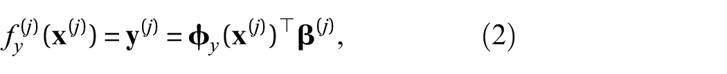
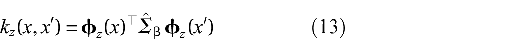
the GP can be expressed as

where
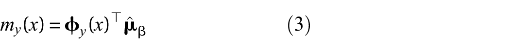
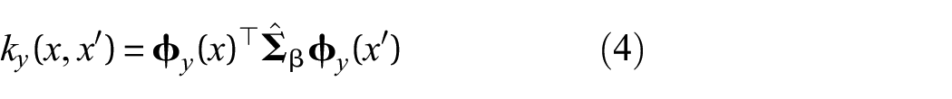
The approach first tries to describe all possible functions by a GP. Second, after determining the mean and covariance function, the GP can be updated by computing the conditional distribution based on currently measured data, that is, data describing the current state of the monitored system. When the mean function

with
and
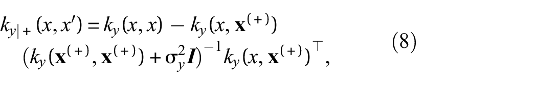
where
Warped GPs
By modeling the system output with a GP, the output is assumed to be normally distributed—presuming it to be defined from negative to positive infinity. This assumption, however, is often not valid as, for example, crack lengths, damage indices, sunlight time, etc., are only defined in the positive domain. For a better treatment of data that is not normally distributed, Snelson et al.
33
introduced warped GPs. The idea is to transform the observed space y onto a latent space z by a so-called warping function

where
Some researchers have already used warped GPs, for example, to predict the power supplies of wind turbines. In contrast to wind speeds, power supplies cannot be assumed to be normally distributed due to the nonlinear correlation between wind speed and power.
34
Therefore, the authors of35–37 utilized warped GPs to predict the power supplies of wind turbines. They used a sum of
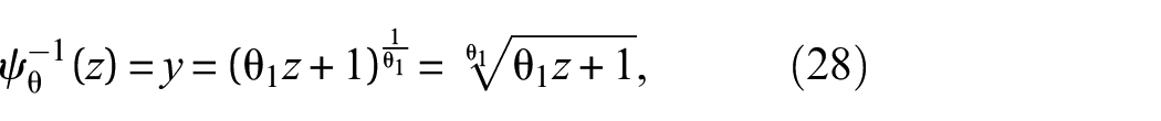
However, if the inverse warping function is not available in closed form, which is the case in the before-mentioned papers, additional complexity arises from numerical approximations. 39 Therefore, one can use, for example, the Box–Cox transformation 40
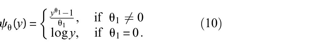
as the warping function. For example, Rios and Tobar 39 utilized a slightly adjusted type of the Box–Cox transformation function and showed its effectiveness on real data, enforcing their predicted yearly sunspot numbers to be strictly positive. A similar application of warped GPs was presented by Gonçalves et al. 41 The authors estimated future sunspot numbers and enforced their predictions to be positive by using an integrated softplus function in their warping function.
Even though these studies show that warped GPs are able to deal with non-normally distributed data, researchers tend to use them rarely. This might be because the warping function introduces additional parameters to the modeling task. These parameters must be optimized in addition to the mean and covariance function parameters. Therefore, one entailed problem is the arising computational complexity by determining not only the mean and covariance function parameters but also the ones of the warping function. Another problem is that after introducing a warping function, an optimizer might find, in fact, a different solution. But the result is not necessarily better, as minimizing the NLL is, in general, a non-convex optimization problem. In order to remove the mean and covariance function parameters, we can derive these functions from previously gathered trajectories. In this way, we significantly reduce the computational complexity and additionally integrate prior knowledge into warped GPs.
Approach
In order to exploit the advantages of warped GPs and the use of basis functions for inferring the GP model quickly from previously collected data, both approaches are combined in the following. For doing so, it is assumed that the warped realizations

and the GP in the latent space as


Note that the GP model is independent of any free parameter
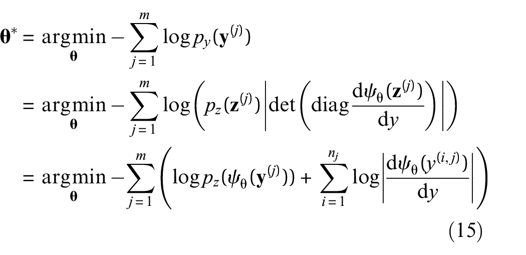
with the given probability density function in the latent space
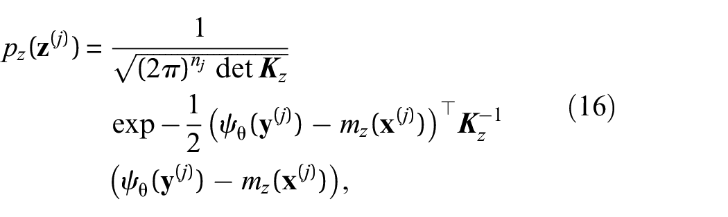
where

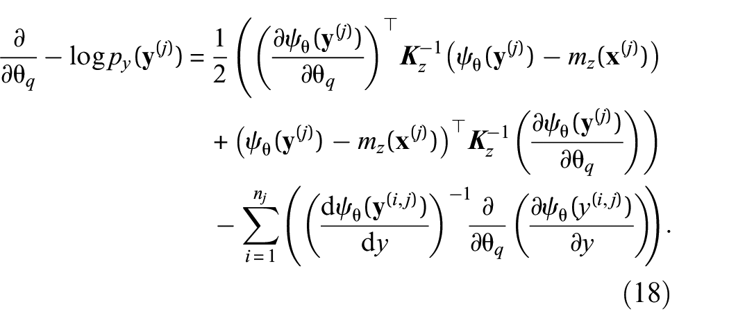
The gradient with respect to the parameter
By transforming the observed data into the latent space, the observation error is warped too. A constant observation error in the observed space
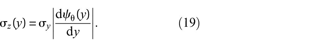
This approximation is particularly accurate if the observation error
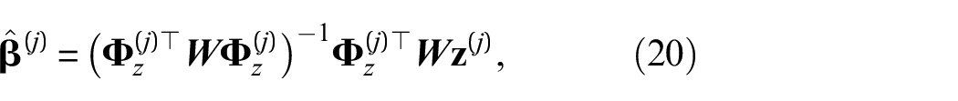
with
and

Now, the mean and covariance function can be determined with Equations (20)–(22) (fitting coefficients) and 12–13 (mean and covariance function) within every iteration step of the warping function parameter optimization. The result of the presented approach is an optimized warping function and a determined GP in the latent space. The observation error
Afterwards, the conditional distribution in the latent space can be computed by substituting
Application to an infinite plate
As a first example, we examine the proposed method on an academic example, a pre-cracked infinite plate, for which the underlying formulas and solutions are known.
Data generation
Considering an infinite plate with a centered crack, the range of the stress intensity factor (SIF)

where a is the crack length and

where
where
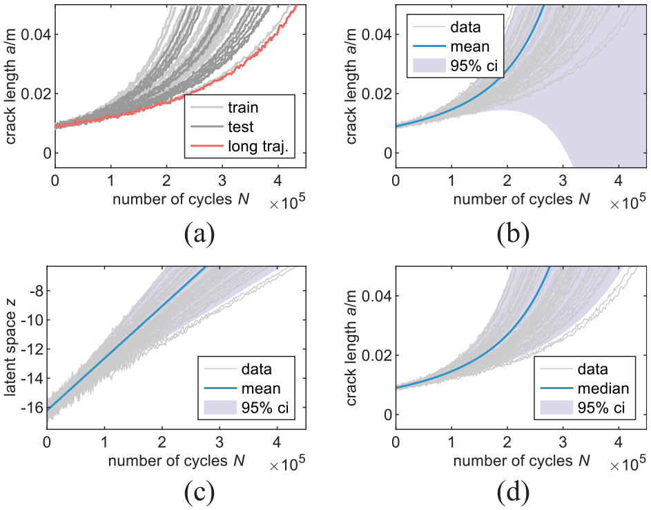
(a) Crack growth trajectories, (b) GP in the observed space, (c) warped GP in the latent space and (d) in the observed space.
Training of GPs
First, a GP without the use of a warping function is trained on 35 trajectories of the simulation data representing previously collected data. A set of polynomial basis functions
In the second case, the warping function in Equation (10) is considered. The free parameter
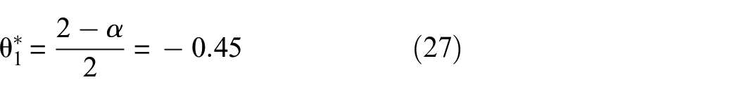
such that the latent space is modeled by a GP with straight lines. In this example, the optimizer leads to a value of
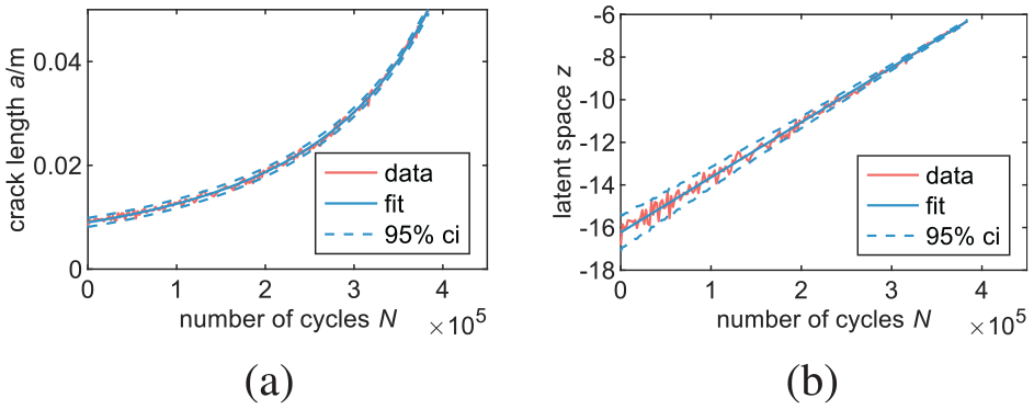
The resulting GP in the latent space and the corresponding warped GP, which is mapped to the observed space by the inverse warping function, are shown in Figures 1(c) and (d), respectively. Figure 1(d) shows that the credible region of the warped GP assumes only positive values. Figure 1(c) additionally shows that the combination of the warping function and the choice of polynomial basis functions with orders 0 and 1 leads to the desired solution. During the optimization process, the optimizer tries, on the one hand, to warp the data such that the trajectories follow a normal distribution in the latent space. On the other hand, the optimization tries to straighten the simulated data in the latent space to fit the presumed basis functions.
Figure 2 shows another effect related to the transformation, which we mentioned at the end of the Approach section. The constant observation error
Observation error in (a) observed space and (b) latent space.
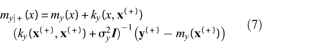
Condition GPs on current crack length data
In the next step, we gradually condition the GPs on currently observed data to update the prediction for an unseen trajectory according to Equations (6)–(8). This is done for the entire test set, even though only one test trajectory is depicted here. Figure 3 shows the GP’s prediction of the longest test trajectory (indicated in red) conditioned on currently observed data. Since the monitoring process is continuous, not all measurements are available from the beginning. The currently available ones are shown in black. In both cases (standard and warped), the credible regions narrow down with more available current data. Figure 3(a) reveals that the standard GP initially updates the mean function so that it becomes negative. This is because the current data has a relatively flat trend which, in combination with the assumed basis functions, results in such predictions. By comparison, the warped GP in Figure 3(b) shows strictly positive predictions. The warped GP is conditioned in the latent space, and the results are afterwards mapped to the observed space by the inverse of the warping function, leading to strictly positive predictions.
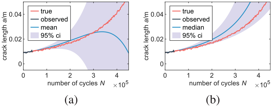
Crack growth prediction for the infinite plate at cycle number 38,000 of (a) GP and (b) warped GP.
In order to compare the two models, the mean negative log-likelihood (MNLL), the mean absolute error (MAE), and the root mean squared error (RMSE) of the test set are quantified. The crack lengths predicted at the trajectory’s last number of cycles for each conditioning step are compared to the latest realized crack length for all metrics. The results are listed in Table 1. For all metrics, the warped GP performs better than the standard GP as it predicts strictly positive crack lengths and resembles the optimal solution (GP with straight lines in the latent space with
Evaluation results for the infinite plate of the standard and warped GP.
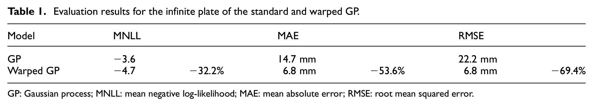
GP: Gaussian process; MNLL: mean negative log-likelihood; MAE: mean absolute error; RMSE: root mean squared error.
As we have seen, utilizing the Box–Cox transformation for warping our data leads to approximations close to the analytical solution for the infinite plate example. However, using this exact type of transformation function results in imaginary numbers if
As presented earlier, we first compute our predictions in the latent space and second map them by the inverse warping function to the observed space. Since the inverse of the Box–Cox transformation reads
we must also ensure that
These constraints limit the applicability of this specific type of Box–Cox transformation. Since the Box–Cox transformation can be useful even in situations where no power transformation can produce normality exactly, 42 it is worth adjusting it. Bickel and Doksum 43 presented the modified Box–Cox transformation function
which was also used by Rios and Tobar.
39
This modification leads to strictly monotonic warping functions over
Ultimately, the infinite plate example reveals the great predictive capabilities of warped GPs. Since the GP is modeled in a latent space, the warping approach is more flexible than standard GPs. The approach enables the prediction of non-normally distributed trajectories, which is especially useful for PHM problems due to their non-negative nature. By contrast, since standard GPs rely on a normal distribution, the possible functions of their conditional distribution can become negative. Yet, one drawback of warped GPs is that the parameters of the warping function need to be optimized, leading to greater computational effort.
Application to an aerospace structure
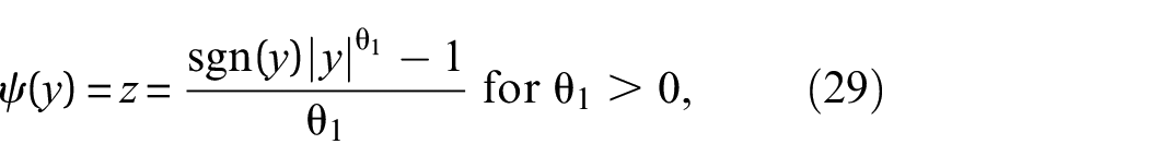
The method proposed in the Approach section is also applied to predict the crack growth in an aluminum panel that resembles a lower section of a civil aircraft wing. The structure is made of the aluminum alloy Al 2024-T351 with Young’s modulus of
(a) Specimen and (b) CAD of the test rig.
The armhole in the center of the structure is usually covered by a lid that is fixed on the smaller holes around it. The armhole allows reaching into the wing to inspect the inner part of the structure with an endoscope. This aerospace structure is prone to fatigue cracks, and it is used to showcase the developed method on warped GPs.
The present section is divided into five parts: First, we describe the experimental setup of the executed fatigue tests. Second, the simulation of multiple crack growth trajectories for generating training data is explained. Third, the generated trajectories are used for training a warped GP according to the proposed method. Fourth, we show how to estimate the current state of the structure, that is, the current crack length, based on measured strain data. And fifth, future crack lengths are predicted by using the trained warped GP and the estimated current crack lengths.
Experimental setup
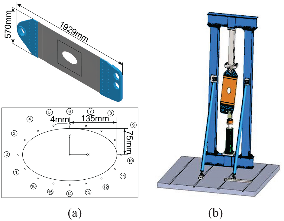
During the fatigue test of the aerospace structure, the load was applied by a hydraulic cylinder at an angle in order to represent the shear stresses in a wing resulting from twisting, see Figure 4(b). The loading program is based on four different flight types, A, B, C, and D, to realistically simulate the forces acting on an aircraft wing, see Figure 5.
Loading program with flight types (a) A and B and (b) C and D.
They consist of 230, 190, 114, and 146 load steps, respectively. The flight types are ordered randomly for the first 100 flights and repeated consecutively afterwards. The occurrences of the different flight types, A, B, C, and D, in the first 100 flights are 55, 15, 20, and 10 times, respectively.
Two equally manufactured specimens, P02T01 and P03T01, were tested with the same loading program. Several sensors were attached to the panel to monitor the structures. They were predominantly positioned according to the method described in Reference.44,45 According to this method, the change of strain regions due to different possible cracks are evaluated with FE analyses. Based on a certain requirement for the change of strain that can be detected by the applied sensors, the positions that satisfy this requirement for every possible crack are determined. Therefore, the method ensures that the deployed sensors are able to detect the occurring cracks. In total, two single strain gauges and three strain rosettes were attached to specimen P02T01 and two single strain gauges and four strain rosettes to specimen P03T01, see Figures 6(a) and (b). For each flight, the strains were measured at every load step.
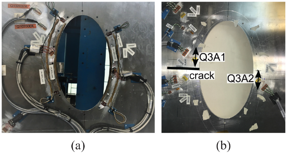
Sensors of (a) P02T01 and (b) P03T01 with the two investigated strain directions Q3A1 and Q3A2.
The experiments were run until final fracture of the structure, see Figure 7. During the experiment, the structure was regularly inspected by test engineers in order to detect cracks and measure their lengths.
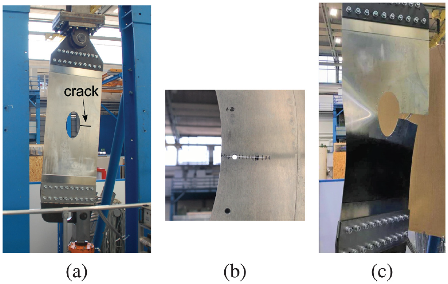
Fatigue process of aerospace structure with (a) intact structure, (b) crack growth, and (c) final fracture.
Generation of training data
The method proposed in the Approach section enables integrating prior knowledge from previously collected degradation trajectories into GPs. As large structural fatigue tests are usually carried out only once, previously measured degradation trajectories are missing. However, due to analytical equations and FE analyses, much of the degradation behavior is understood a priori. In order to integrate this knowledge into GPs, degradation trajectories are gathered by conducting virtual simulations. First, the fatigue life and second, the crack growth are computed to simulate the structure’s degradation. The entire simulation process is schematically shown in Figure 8.
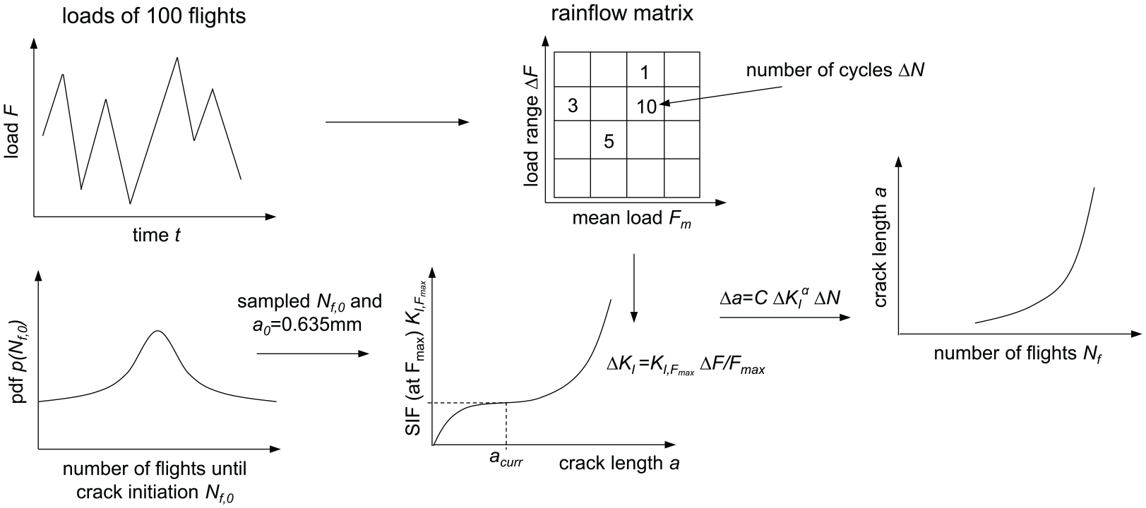
Schematic representation on how the crack growth in the aerospace structure is simulated where
Fatigue life
First, an FE analysis is carried out to quantify the stresses in the structure. Two local hot spots are found at the small holes 5 and 6 on the side toward the armhole. In the following, we assume the crack to start at hole 6. However, the methodology can also be extended to consider cracks starting from multiple spots by modeling a mixture of GPs.
By applying rainflow counting and the Haigh diagram to the computed stress at hole 6, the stresses for the entire loading program can be mapped to amplitude stress blocks with a constant stress ratio of
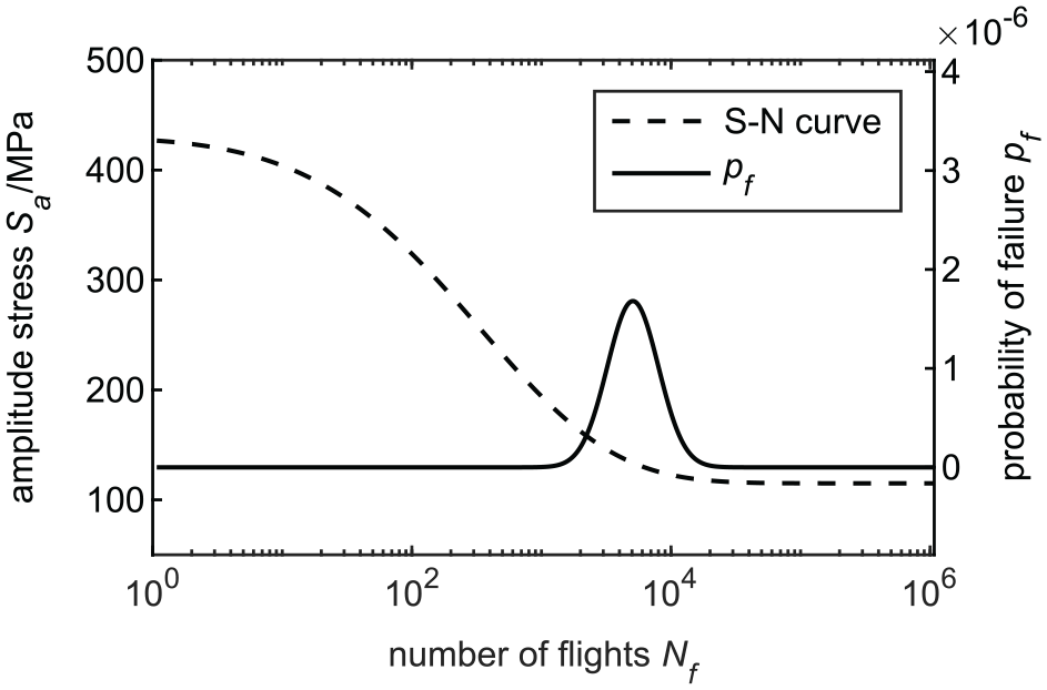
S–N curve and log10 normal distribution for the present loading program.
Crack growth
Second, the crack growth in the structure is evaluated. To quantify the relationship between the SIF and the crack length a, multiple crack computations are evaluated using the extended finite element method (XFEM).47–49 The crack is assumed to first propagate toward the armhole (crack length
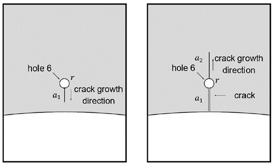
Assumption for crack propagation where crack 1 first propagates toward the armhole (left) and crack 2 to the edge of the specimen afterwards (right).
In total, 382 XFEM computations (static analyses), see Figure 11(a), with different crack lengths are evaluated to quantify the relationship between a and
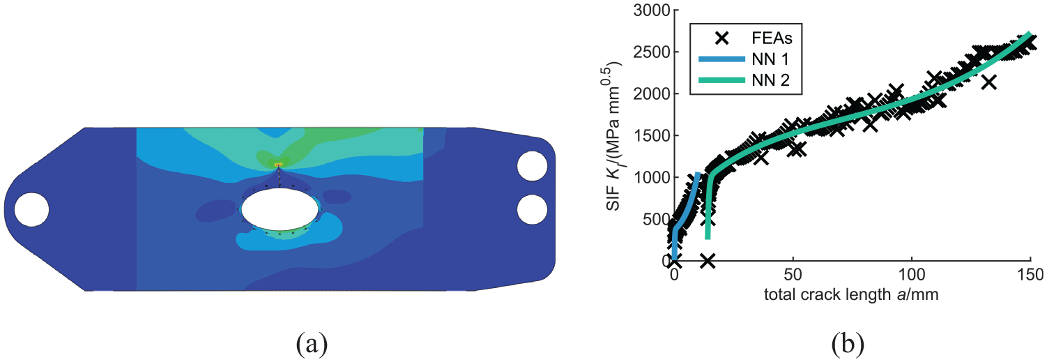
(a) XFEM computation and (b) trained NN.
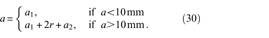
In this paper, we define the total crack length a as
As Pfingstl et al.,
44
an initial crack length of

In order to reduce computational time, the crack growth computations are simplified by applying rainflow counting
51
to the load steps of 100 flights to compute the load ranges and using
Figure 12 shows the computed degradation trajectories. Note that the step in each trajectory results from the two different cracks,
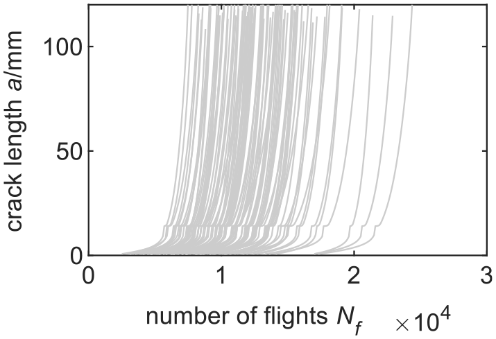
Computed degradation trajectories.
Training of GP
A warped GP can now be trained on this simulation data set according to the method proposed in the Approach section. By using simulation data for training, however, one has to be sure that the simulations are correct. When there are doubts about whether the simulations represent the experiment well, they should be verified based on experiments before using them as the training set.
For this example, the modified Box–Cox transformation of Equation (28) is used as the warping function and a polynomial of degrees 0 and 1 (intersection and slope) as basis functions. Therefore, the optimizer tries again to achieve not only a normal distribution in the latent space but also straight lines. The optimized solution is
Figures 13(a) and (b) show the training data and the determined warped GP in the observed and the latent space. It can be seen that the trajectories are almost straight lines in the latent space. Moreover, the mean function and the credible region in the observed space assume only positive values which is in agreement with the physics. Figure 13(a) depicts the prediction before any data of the monitored structure is available.
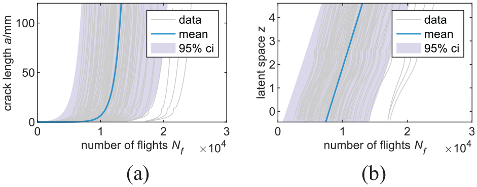
Trained GP in (a) the observed space and (b) the latent space.
Estimation of current states
In order to update the trained GP, the current state of the system has to be observed. As the present GP is based on crack growth data, the current crack length must be determined. In the present study, the applied strain gauges are used to determine the current crack length. With Bayes law, the crack length a can be inferred from the measured strain
where
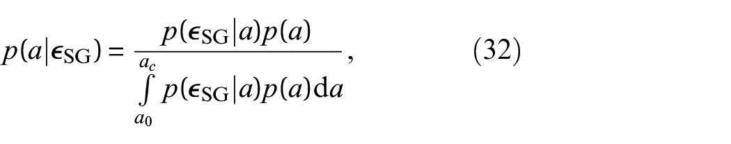
Additionally assuming the prior
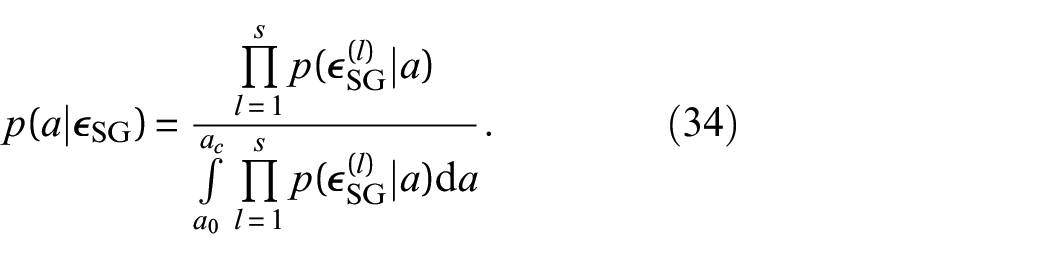
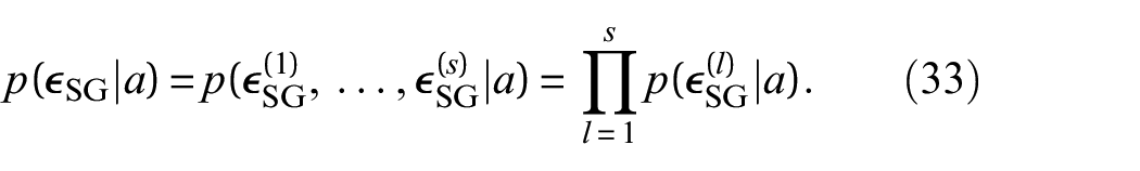
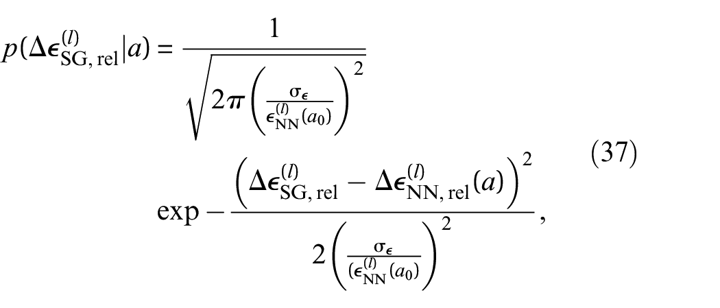
In order to be able to use Equation (34), the likelihoods
In order to cancel out the bias term which might emerge from the difference between the FE analysis and the real measurement, only the relative change of strain due to a crack
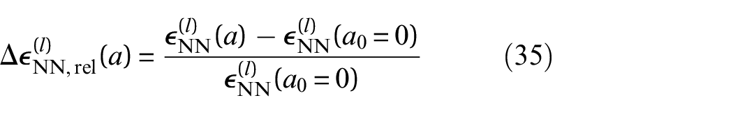
and
are considered. Since settlement effects happen at the beginning of each test, the measurement of flight 500 is used as
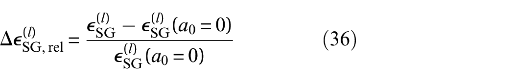
Figures 14(a) and (b) show the absolute strains for two strain gauge positions computed by FE analyses (black crosses). Additionally, the blue lines indicate the trained NNs. As mentioned before, we do not use the absolute values since there might be a bias term between the FE analysis and the measurements. Therefore, we compute the relative change of strains shown in Figures 14(c) and (d). Moreover, the change of strains for two different sensor positions (Q3A1 and Q3A2) over the number of flights are displayed in Figures 14(e) and (f). By using the strain’s relative change, all lines begin at zero, canceling the bias term. The figures also show that if the crack grows, the strain becomes smaller at the position of sensor Q3A1 and larger at Q3A2. Furthermore, Q3A1 indicates a very sensitive behavior for small cracks and Q3A2 for larger ones. This can be explained by looking at Figure 6(b). The figure shows that the crack occurs close to position Q3A1 and cuts the load path so that smaller strains are measured. By contrast, position Q3A2 lies on the opposite side of the crack. If the crack starts growing, no significant change of the strain is measured. However, once the crack is long enough, the load path is shifted to the side of position Q3A2, increasing the measured strain.
Trained NNs on absolute strains for positions (a) Q3A1 and (b) Q3A2. NNs representing the relative change of strains for (c) Q3A1 and (d) Q3A2. Measured change of strains over the number of flights for (e) Q3A1 and (f) Q3A2.
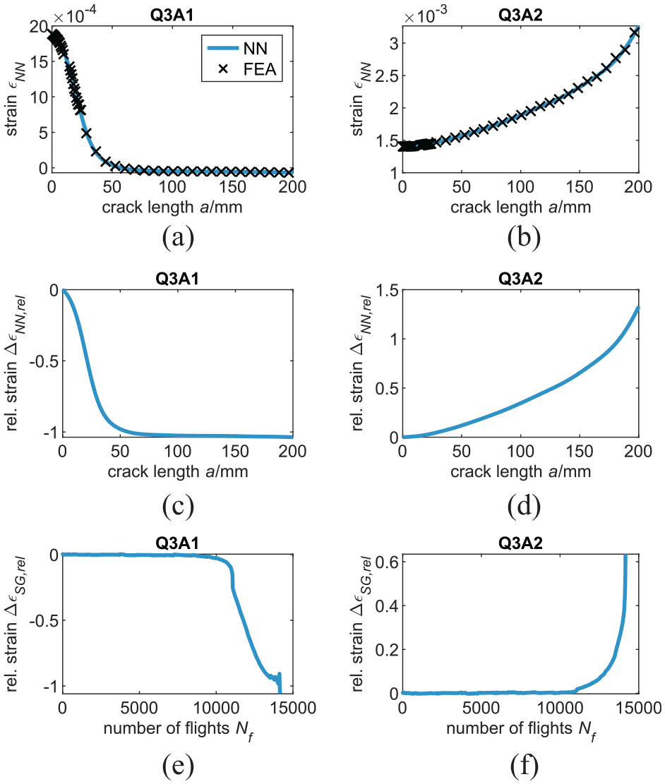
The relative change of strain for every flight is computed by the relative change of the strain–force slope shown in Figure 15. While the change of the slope for position Q3A1 can be well distinguished for smaller numbers of flights (smaller cracks), position Q3A2 is better for indicating the crack lengths at larger numbers of flights (larger cracks), see Figure 15(a) and (b), respectively.
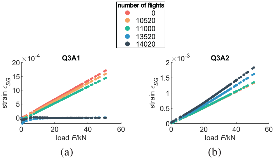
Measured strains for different flights at position (a) Q3A1 and (b) Q3A2. The color indicates a certain number of flights.
By using the relative change of strain instead of the absolute values, the likelihood becomes
which is used instead of

and its variance by
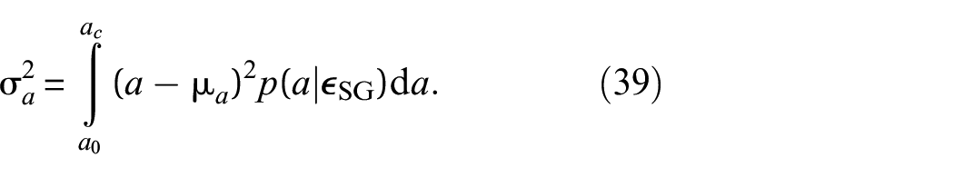
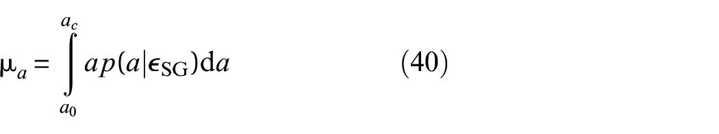
Figure 16(a) and (b) show the crack lengths inferred from the measured strains and the corresponding crack lengths visually inspected by test engineers for both specimens. It can be seen that the inferred crack lengths for P03T01 closely match the inspected ones (
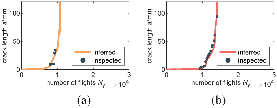
Inferred crack lengths and visual inspections for specimen (a) P02T01 and (b) P03T01.
As the P03T01 specimen was tested after P02T01, the test engineers were already familiar with the type of structure and were, therefore, able to measure the crack lengths more accurately. Still, both crack growth behaviors are very similar to the inspected ones, and are close to the simulations in terms of locations, numbers, and crack growth rate.
Prediction of future states
Although Figures 16(a) and (b) show the entire trajectories of the inferred crack lengths, during the test, the crack length is only partially known, that is, from
Figures 17(a) to (h) show the updated predictions for specimens P02T01 and P03T01 at different time states. Initially, the GP’s prediction is entirely based on the knowledge gained from analytical equations and FE analyses. Once a crack length greater than
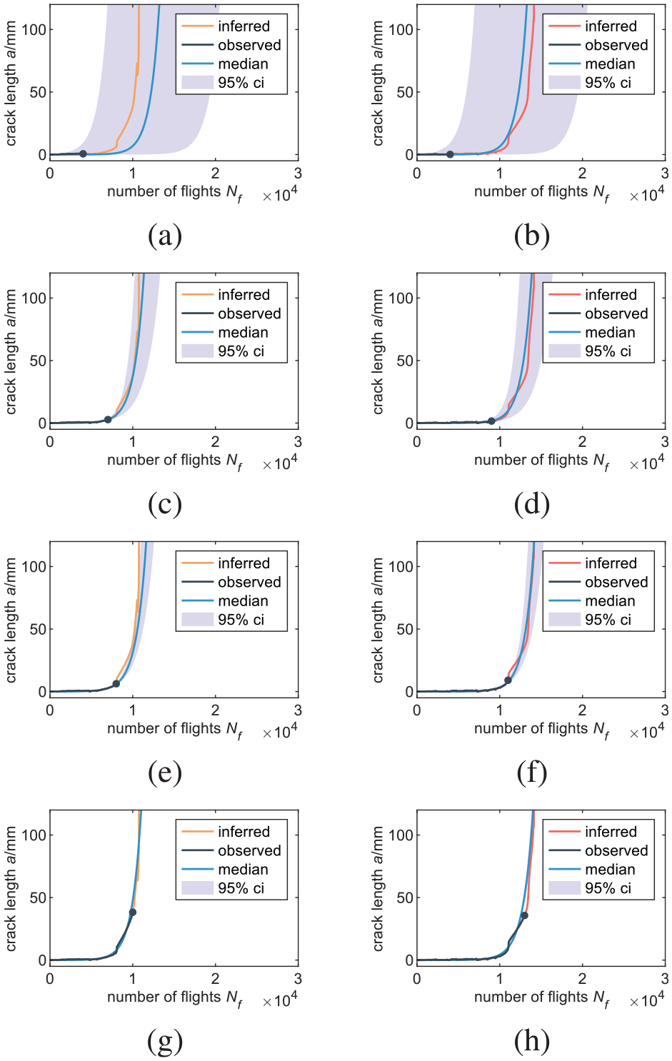
GP predictions for specimen P02T01 at number of flights equal to (a) 4000, (c) 7000, (e) 8000, and (g) 10,000, and for specimen P03T01 at (b) 4000, (d) 9000, (f) 11,000, and (h) 13,000 flights.
Discussion
Warped GPs
As demonstrated for an infinite plate and an aerospace structure, the proposed approach on warped GPs can even handle data that is not normally distributed. In both cases, introducing a warping function leads to predictions that assume strictly positive values. This is in agreement with the physics since crack lengths can only be positive. The approach reproduces the analytical solution for problems without an observation error and leads to a close approximation (
Simulations
Prior knowledge in the form of degradation trajectories is often rare, especially if the mechanical system is large and expensive. Using analytical and FE-based simulations can produce valuable information that can be incorporated into GPs by the presented approach, see section Application to an aerospace structure. By splitting the approach into two parts, (1) training a GP on previous data and (2) computing the conditional distribution for updating the prediction based on currently monitored data, allows rapid predictions that may be evaluated online. Nevertheless, incorrectly executed simulations resulting, for example, from the use of incorrect parameters, can lead to weak predictions. Therefore, the simulation and its parameters, as well as their uncertainties, should be well known. To avoid overconfidence, it is better to assume overly large variances than variances that are too small since there might be sources of uncertainties that are not known in advance.
Hidden state of the system
After the GP is defined by its mean function and covariance function, it can be conditioned on current data. The current state of the system, however, is often hidden. Therefore, the present paper shows how to infer the crack length from strain data. Based on the coefficient of determination, the resulting crack lengths using Bayesian inference match the crack lengths measured during inspections with
Conclusion
The present paper proposes a PHM algorithm that is based on GPs. It is successfully applied to an infinite plate and an aluminum aerospace structure in order to predict crack growth. The established model predicts not only the crack length for every future time step but also its credible intervals. By describing the crack length as a random variable, different credible regions, for example, a
The proposed algorithm is based on warped GPs. Using warped GPs reduced the MAE by 53.6% and the MNLL by 32.2% for the infinite plate example investigated in this paper. It also leads to strictly positive predictions for crack lengths, which is in accordance with the physics. Furthermore, the proposed approach can quickly integrate prior knowledge in the form of several previously generated degradation trajectories. Since prior knowledge is often only available in terms of analytical equations and FE analyses, the present paper shows how to generate them for an aerospace structure prone to fatigue cracks. In general, the simulations must be trustworthy and might be verified before using them. Therefore, the approach is currently limited to crack growth predictions for isotropic materials. In future research work, it would be interesting to apply a similar approach to composite structures.
In order to update the GP’s prediction, the current crack lengths are inferred from strain data, which agree well with the visually inspected ones. Ultimately, the estimated and predicted crack lengths can be used to compute the probability of failure and therefore to better schedule maintenance tasks.
Footnotes
Acknowledgements
We thank Prof. Dr. Kochenderfer from the Department of Aeronautics and Astronautics of Stanford University for the valuable discussion.
Declaration of conflicting interests
The author(s) declared no potential conflicts of interest with respect to the research, authorship, and/or publication of this article.
Funding
The author(s) disclosed receipt of the following financial support for the research, authorship, and/or publication of this article: This research was funded by the Federal Ministry for Economic Affairs and Energy based on a decision by the German Bundestag in the national aeronautics program LuFo V as a part of the research project Strubatex.