Sage Journals: Discover world-class research

Abstract

Permanently installed ultrasonic sensors have found increasing applications in the field of structural health monitoring (SHM), in particular with respect to thickness measurement and corrosion monitoring. As ultrasonic velocity is temperature dependent, the state and temperature distribution of a component contribute to much of the measurement uncertainties of an ultrasonic SHM system. On the other hand, the temperature dependency of ultrasonic velocity has also led to various temperature sensing methods for measuring temperature distributions within solid materials. While conventional ultrasound-based techniques can measure either a component’s thickness at a given temperature, or the internal temperature distributions at a given component thickness, measurement fluctuations and drifts can occur if both variables are set to change simultaneously. In this study, we propose a dual-wave approach to overcome the limitations of the existing methods. ‘Co-located’ shear and longitudinal pulse-echo measurements are used to simultaneously track the thickness change and through-thickness temperature variation of a steel plate in complex environmental conditions. Results of the verification experiments showed that, in the given conditions, the proposed dual-wave correction method could reduce thickness measurement uncertainties by approximately a factor of 5 and eliminate 90% of the drift in temperature predictions.

Keywords

Ultrasonic corrosion monitoring thickness gauging temperature prediction temperature compensation simultaneous monitoring dual-wave correction

Introduction

Motivation

Ultrasonic testing has been widely used in the field of non-destructive testing and structural health monitoring (SHM) for its non-destructive nature and relative ease of implementation. Two of its most widely used applications are thickness gauging and temperature sensing. While many research studies have addressed wall thickness loss or subsurface temperature sensing separately, simultaneously monitoring the two variables presents a particular challenge to existing ultrasonic monitoring systems.

For thickness gauging, a conventional ultrasonic transduction system excites either shear or longitudinal ultrasonic waves in the component being monitored. Component thickness can then be inferred based on the recorded time-of-flight (ToF) of ultrasonic waves. However, as the propagation velocity of ultrasonic waves is temperature dependent, the performances of ToF based thickness gauging and SHM systems can be severely affected by temperature fluctuations in the environment.^1,2 If the temperature within a system is uniform, highly accurate thickness tracking can be performed with surface temperature measurement and simple temperature compensation methods. In a laboratory environment, ultrasonic thickness monitoring systems can achieve ‘sub-micrometre’ level accuracy if strict temperature controls are in place.^3–5 However, the performance of such a system may deteriorate significantly in industrial settings, where temperature fluctuations cause non-uniform subsurface temperature gradient within the system.^6,7 Properly compensating for the subsurface temperature gradient is difficult due to the scarcity of information that can be obtained with conventional, non-invasive thermometry techniques.

On the other hand, by employing the temperature dependency of ultrasonic wave velocities, various ultrasonic thermometry techniques have been proposed for estimating subsurface temperature distributions.^8–12 The authors have previously compared two ultrasound-based methods for predicting subsurface temperature distributions in solid media.¹³ However, to the best knowledge of the authors, all of the previously proposed methods assume that the thickness of the component (i.e. the length of the wave path) are known and remain constant. If the component thickness starts to vary due to corrosion or erosion, the ultrasonic temperature predictions will drift, resulting in increasing prediction errors.

To summarise, the conventional, single-wave mode thickness gauging/temperature sensing techniques cannot differentiate if the changes in ToFs of the reflected ultrasonic waves are caused by temperature fluctuations or wall thickness loss. This is because not enough information can be extracted from the received ultrasonic signals of a single-wave type. To overcome this limitation, we propose a dual-wave (i.e. shear and longitudinal waves) approach to simultaneously monitor the two variables. This is an extension of our previous work on temperature reconstruction only.¹³ Here, we seek to apply the information that is gained from the subsurface temperature distribution to improve the accuracy and robustness of conventional ultrasonic thickness gauging systems, and at the same time address the inherent limitation of the temperature sensing method.

Paper structure

This paper is structured as follows: The section ‘Measurement Principles’ first presents the working principles of conventional ultrasonic thickness gauging and temperature sensing methods, which are the baselines of this study. We then investigate the effects of component thickness change on ultrasonic temperature predictions. The dual-wave prediction method is then proposed and its process flowchart is presented at the end of the section. The section ‘Numerical Simulation’ first describes the problem being considered in this study and the procedures of generating simulation inputs. This is followed by three case studies that demonstrate the performances of the dual-wave method at different conditions. The procedures and results of the verification experiment are described in the subsequent section ‘Experimental Verification’. We also discuss discrepancies between simulation and experimental results, and highlight potential limitations of the proposed method. Lastly, the main findings of the study are summarised in the concluding section.

Measurement principles

Ultrasonic thickness gauging and temperature compensation

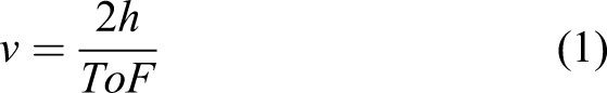
Figure 1 shows sample ultrasonic shear and longitudinal wave signals, which were obtained on a 30 mm-thick mild steel (080A15/EN32B) specimen. The shear and longitudinal waves were excited and sampled simultaneously by two independent piezoelectric PZT transduction systems. The ToF of the ultrasonic reverberations between interface-A and -B can be determined by measuring the time interval between multiple echoes. If component thickness, h, is known, the propagation velocity of ultrasonic waves in the material can be calculated using

v = \frac{2 h}{T o F}

(1)

Figure 1.

Sample ultrasonic measurements. Blue trace: shear (S) wave signals. Brown trace: longitudinal (L) wave signals.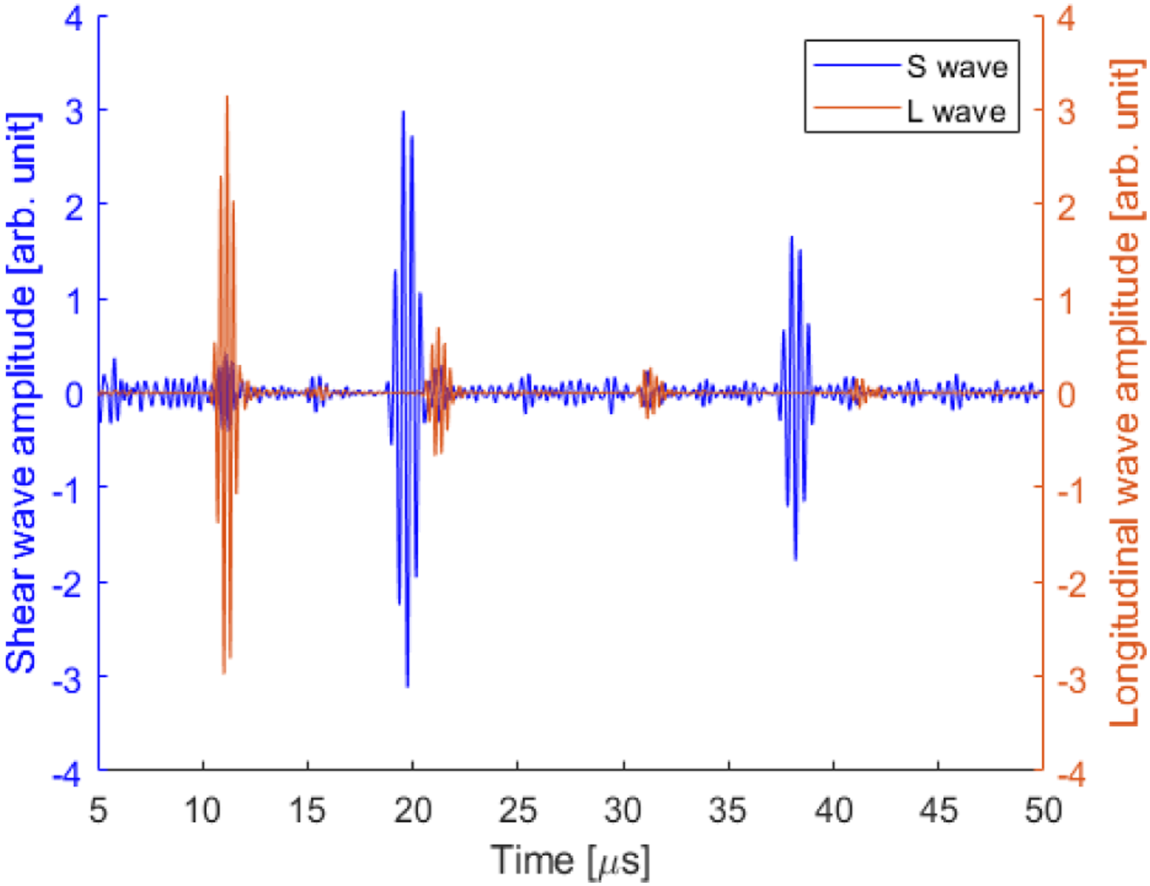

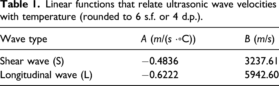
Ultrasonic velocity is known to be temperature dependent. Figure 2 plots the velocity-temperature (v-T) relation of shear and longitudinal waves in mild steel (080A15/EN32B). The relations were obtained experimentally by gradually cooling the specimen in a controlled environment. The temperature distribution within the specimen is assumed to be uniform during the process. Although the underlying mechanisms that relate ultrasonic velocity and temperature are complicated, the velocity-temperature relation can often be approximated using relatively simple polynomial functions. In this case, a first order linear function is adopted for each of the shear and longitudinal waves, respectively. Coefficients A and B of Equations (2) and (3) relate ultrasonic velocity, v with temperature, T. The subscript s and l indicate the association of the coefficients with shear and longitudinal waves, respectively. The values of coefficients A and B are summarised in Table 1

v_{s} (T) = A_{s} T + B_{s}

(2)

v_{l} (T) = A_{l} T + B_{l}

(3)

Figure 2.

Velocity-temperature (v-T) relations for shear (S) and longitudinal (L) ultrasonic waves.

Table 1.

Linear functions that relate ultrasonic wave velocities with temperature (rounded to 6 s.f. or 4 d.p.).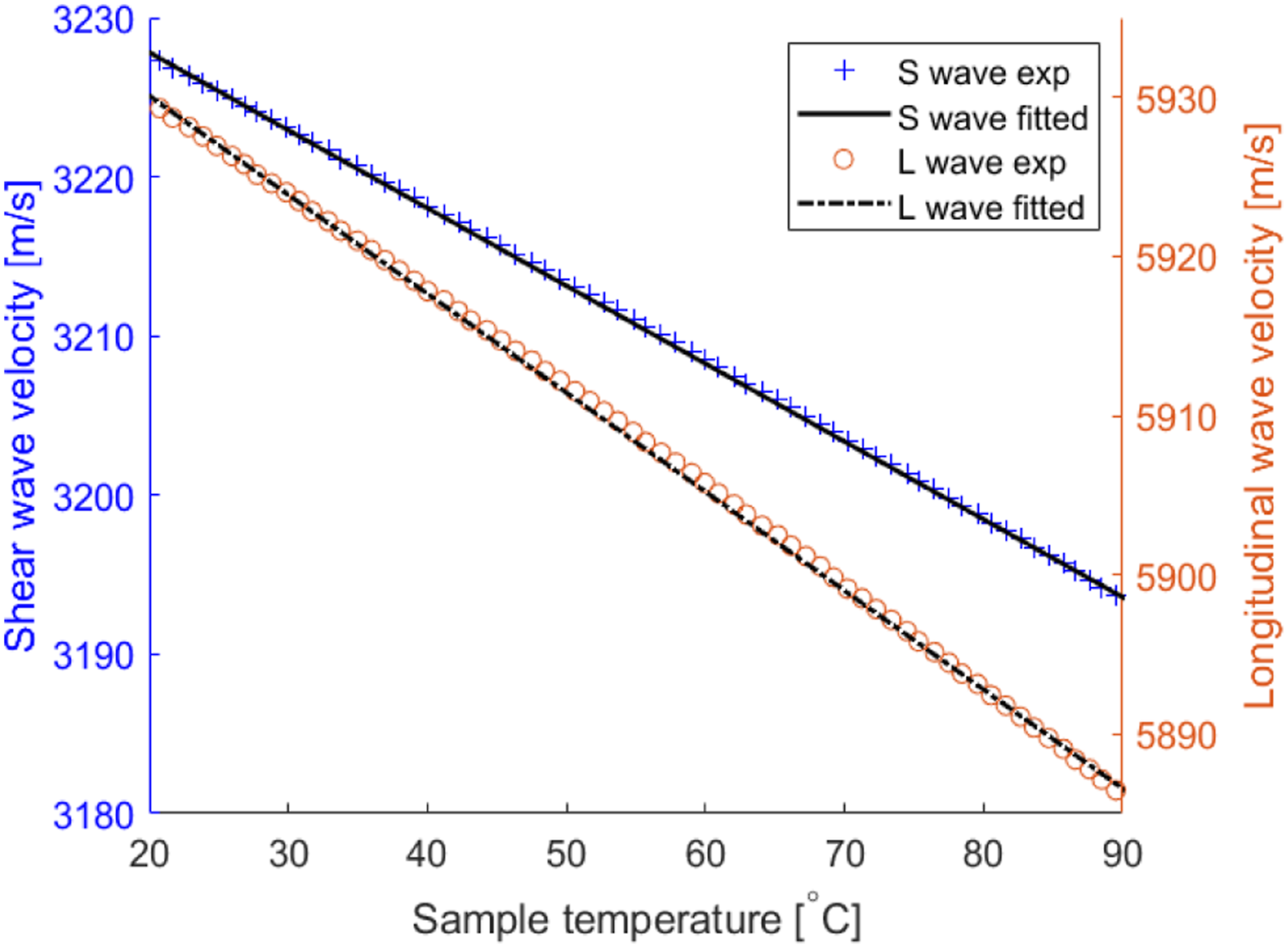

Wave type	A (m/(s ⋅◦C))	B (m/s)
Shear wave (S)	−0.4836	3237.61
Longitudinal wave (L)	−0.6222	5942.60

If both ToF and temperature-compensated velocity are known, the thickness prediction, h_p, of the component can be obtained using Equation (4)

h_{p} = \frac{1}{2} v (T) \cdot T o F

(4)

It is worth noting that in this study, a constant value of h is used in Equation (1) to calculate the ultrasonic velocities at different temperatures (Figure 2). Therefore, it may seem that thermal expansion induced thickness changes are ‘neglected’ in the calculation. However, the effect of thermal expansion has been accounted for implicitly in the shown v-T relations as experimentally measured ultrasonic ToF already includes the contribution of thermal expansions of the material. Although it is possible to consider thermal expansion explicitly in the calculation process, this will result in an additional prior information being required and uncertainties associated with the accuracy of the thermal expansion coefficient will add further complication to the final predictions. Another important implication of this approach is that the values of thickness gauging obtained using the v-T relations refer to the component thickness measured at a constant reference temperature rather than at the actual temperature conditions. This applies to both the single-wave temperature-compensated thickness predictions and the dual-wave thickness predictions presented in this paper.

Ultrasonic temperature prediction by inverse-thermal-modelling

For a 1D system, the temperature distribution of the system during the time-dependent unsteady state can be modelled by solving the 1D heat diffusion equation

\frac{\partial T}{\partial t} = α \frac{\partial^{2} T}{\partial t^{2}}

(5)

where α represents the thermal diffusivity of the material.

To solve Equation (5), the initial temperature distribution of the system and the two boundary values need to be known. In practice, however, temperature measurement is only available at one end of the system (e.g. exterior surface of a pipe) whereas the temperature at the other end (e.g. the pipe interior surface) is unknown due to limited access. With ultrasonic thermometry, the pipe interior surface temperature and therefore, the entire temperature profile across the component thickness/along the wave path can be obtained by iteratively searching for the unknown boundary value until the resulting ToF of ultrasonic waves travelling through the temperature profile is consistent with the measured ToF. By repeatedly performing this process, the temporal-spatial temperature variations within the system can be obtained from a continuous stream of ultrasonic measurements. This is known as the inverse-thermal-modelling (ITM) approach of ultrasonic temperature inversion, which is described in more detail in our previous work.¹³

In addition, since the ITM approach is a physics-based inversion method, it can be applied to either longitudinal or shear wave measurements to obtain two independent temperature predictions, T_s (x, t) and T_l (x, t). If the longitudinal and shear ultrasonic waves propagate through the same system with identical thickness and temperature profile, these two predictions should be identical.

Effects of thickness change on ultrasonic temperature predictions

To investigate the effect of thickness change on ultrasonic temperature predictions, let us first consider a simplified case when the temperature distribution across component thickness is uniform. In this case, the component temperature can be inferred from a transformation of Equations (1) and (2)/(3) and the same value should be obtained whether the shear or longitudinal wave measurements are used

T = \frac{2 h}{A_{s} T o F_{s}} - \frac{B_{s}}{A_{s}} = \frac{2 h}{A_{l} T o F_{l}} - \frac{B_{l}}{A_{l}}

(6)

However, when the incorrect component thickness is assumed in Equation (6), that is, h′ = h + δh, the temperature prediction obtained from longitudinal wave ToF, $T_{l}^{'}$ , can be different from that of the shear wave ToF, $T_{s}^{'}$ . The difference between the two values can be expressed as

T_{l}^{'} - T_{s}^{'} = \frac{δ h}{h} (\frac{B_{l}}{A_{l}} - \frac{B_{s}}{A_{s}})

(7)

where δh represents discrepancies between the actual component thickness and its assumed value.

Hence, for non-zero values of δh, the shear and longitudinal wave temperature predictions will be different if $\frac{B_{l}}{A_{l}} - \frac{B_{s}}{A_{s}} \neq 0$ .

This gives the proposed dual-wave method the sensitivity to differentiate between ToF changes due to thickness variation and temperature fluctuation. The same principle also applies to ultrasonic temperature predictions using the ITM method, as a non-uniform temperature profile can be discretised into multiple elements with uniform temperature.

Flowchart of the dual-wave prediction method

Figure 3 shows the flowchart of the proposed dual-wave (DW) method for simultaneously monitoring thickness and through-thickness variations of a component. Material properties such as the v-T relations and thermal diffusivity are required as prior information. Component thickness and the internal temperature distribution within the system are also assumed to be known. A common initial temperature condition will be uniform temperature distribution at steady state. Once the programme is initiated, ToF measurements of the shear and longitudinal waves, $T o F_{m, s}$ and $T o F_{m, l}$ , are acquired continuously. In this study, the measuring interval for simulation and experimental studies are set to 4 seconds. The shear and longitudinal ToF measurements then feed into the ITM temperature prediction subroutines separately, which outputs two independent temperature predictions, T_s (x, t_n) and T_l (x, t_n). If the maximum difference between the two temperature prediction T_s (x, t_n) and T_l (x, t_n) is larger than a temperature discrepancy threshold, ϵ_T, it suggests that the thickness of the component has deviated from its assumed value and the thickness correction subroutine is triggered. The thickness of the component is adjusted based on the relative magnitude of the two ultrasonic predictions. The updated thickness value is then fed into the ITM subroutines to obtain two new sets of temperature predictions. This process is performed iteratively until a suitable thickness value that satisfies max |T_s − T_l| < ϵ_T is found. Then, the programme either proceeds to the next time instance or outputs the temperature and thickness predictions.

Figure 3.

Flowchart of the proposed dual-wave prediction method for simultaneously monitoring component thickness and through-thickness temperature distribution. ϵ_T denote a pre-specified temperature prediction discrepancy threshold, which triggers the thickness correction subroutine. Δh represent thickness correction increment/decrement.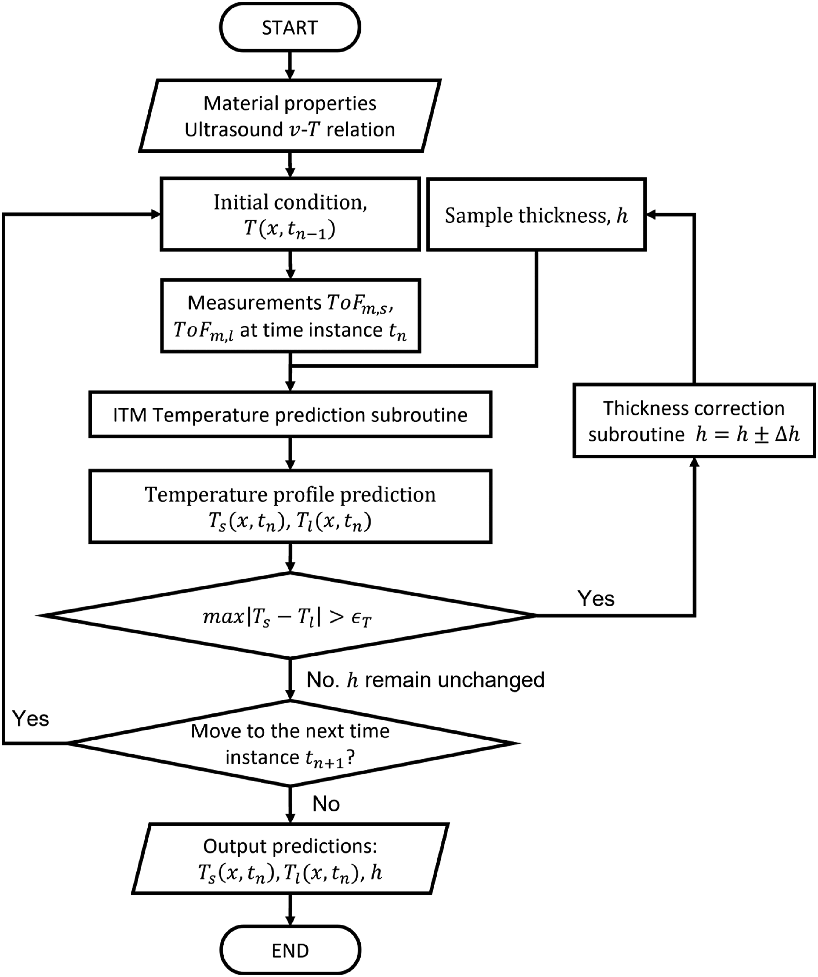

In addition, since any potential discrepancies between the shear and longitudinal temperature predictions using the dual-wave method are kept below an acceptable level (ϵ_T), the average value of the two predictions will be used as the output of the dual-wave temperature prediction.

Numerical simulation

Problem illustration

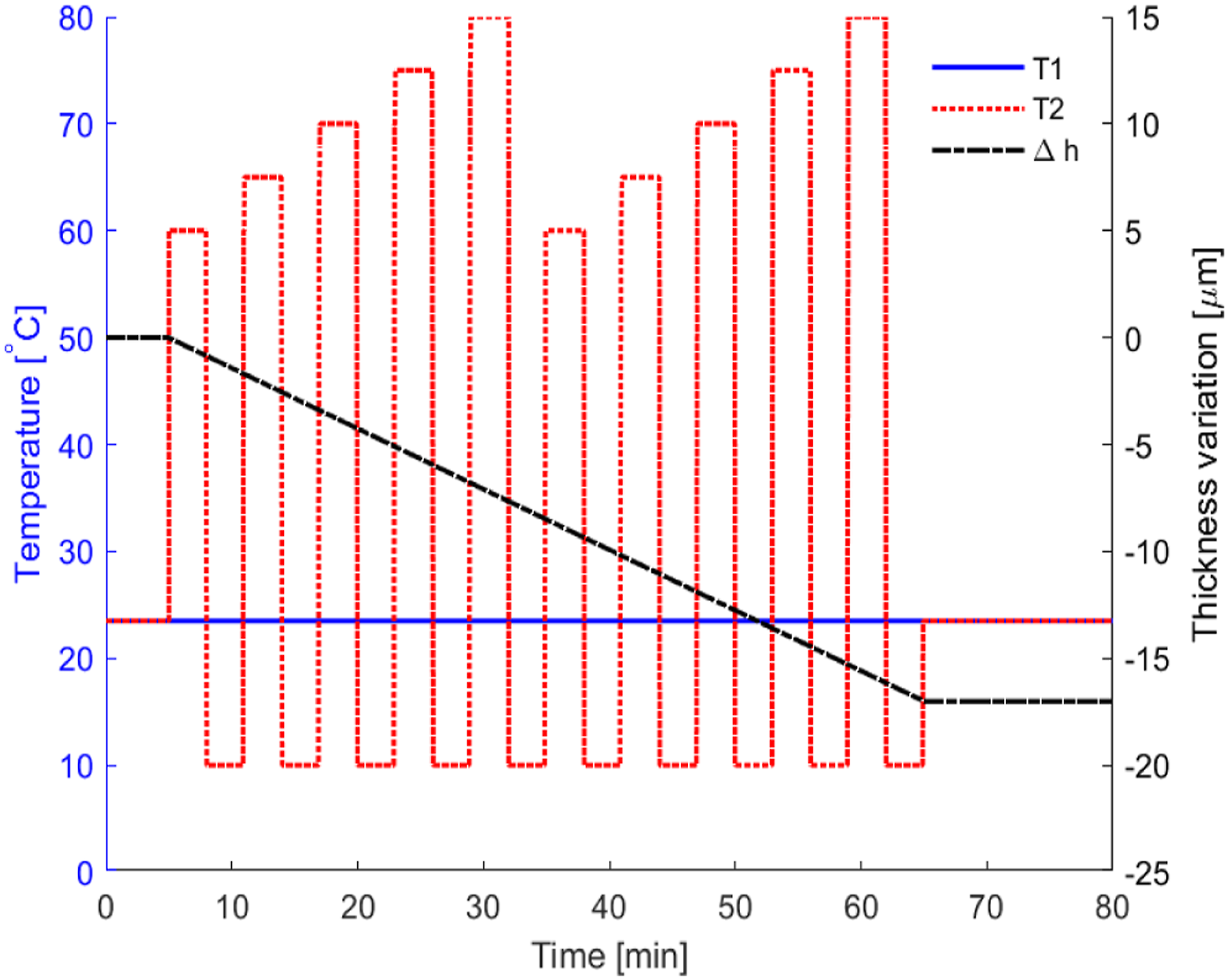
Figure 4 presents schematics of a typical scenario considered in this paper. A 1D system (e.g. a steel plate or pipe wall) separates two media of vastly different conditions. Ultrasonic and temperature sensors are installed at Interface-A (e.g. the exterior surface of a pipe) only due to limited access to Interface-B. While the temperature T1 of Medium-1 is held constant at room temperature, the temperature T2 of Medium-2 fluctuates between 10°C and 80°C, thereby creating a constantly varying temperature gradient within the system. Meanwhile, corrosion of the component at interface-B results in thickness loss of −17.0 μm/hr. Figure 5 presents a graphical illustration of the imposed conditions in the simulation.

Figure 4.

Problem illustration: a 1D solid structure experiences both temperature fluctuations and wall thickness loss.

Figure 5.

Graphical illustration of the boundary conditions of the simulation. T1: temperature of medium-1 (air). T2: temperature of medium-2 (liquid). Δh: component thickness variation.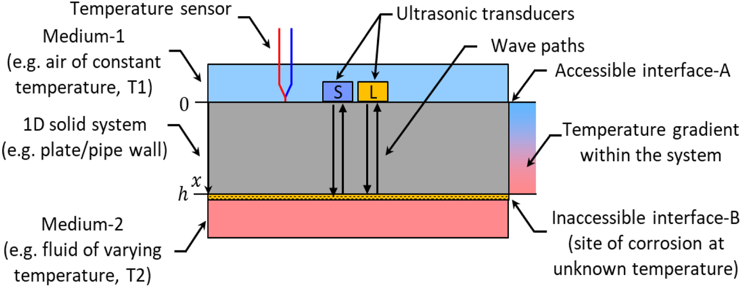

Data generation

Although it is possible to model temperature dependent wave propagation problems with finite element software, a simplified approach was adopted here by focussing on the effects of temperature variations and thickness changes on ToF of the reflected waves.

An energy balance approach¹⁴ is used to define the convective heat transfer at Interface-A and -B while the temporal variations of the temperature distribution of the solid system are modelled by using an explicit finite difference scheme to solve the 1D heat diffusion equation. The detailed implementation of the thermal-modelling is presented in Zhang et al.¹³ Once the internal temperature distribution is known, the velocity-temperature relations of Equations (2) and (3) can be used to determine the ultrasonic velocity profile along the wave path. In this case, Equation (8) is used to calculate the values of ToF for shear and longitudinal waves along a discretised 1D wave path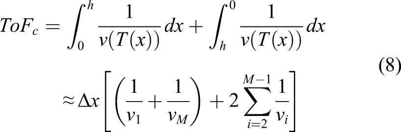

\begin{array}{l} T o F_{c} = \int_{0}^{h} \frac{1}{v (T (x))} d x + \int_{h}^{0} \frac{1}{v (T (x))} d x \\ \approx Δ x [(\frac{1}{v_{1}} + \frac{1}{v_{M}}) + 2 \sum_{i = 2}^{M - 1} \frac{1}{v_{i}}] \end{array}

(8)

where Δx is the grid size and the subscript i for i = 1 to M represent the spatial location of the discretised nodes in x.

To simulate corrosion-induced thickness loss of the component, the dimension of the system is adjusted at the end of each time step of the thermal-modelling by scaling the grid size of the finite difference scheme, Δx. The temperature distribution modelling and thickness adjustment are implemented independently such that the thickness variations neglect thermally induced changes.

Other than the ToF data, the temporal variations of the specimen thickness and temperature distribution are also sampled at a constant interval of 4 s, these will serve as the ‘ground truth’ to assess the performances of the ultrasonic dual-wave correction method. Once the required input data are generated, they are fed into the proposed prediction algorithm. Three case studies are designed to demonstrate the capabilities of the proposed method under different conditions.

Conventional single-wave prediction

We first simulated a baseline case that demonstrates the limitations of conventional single-wave ultrasonic temperature and thickness prediction methods to the readers.

In subplot (a) of Figure 6, ultrasonic thickness predictions based on a single shear- or longitudinal-wave are compared to the true variations. Residuals (errors) of the thickness predictions are shown in the subplot (b). As shown in the graphs, although temperature-compensated velocities (Equations (2) and (3)) have been used for thickness prediction, the conventional temperature compensation method based on exterior surface temperature neglects subsurface temperature distributions within the component. As a result, in the single-shear-wave (SSW) and single-longitudinal-wave (SLW), thickness predictions fluctuate around the true values as the thermal cycles induce subsurface temperature gradients. Residuals as large as ± 14 μm can be observed during the transient periods.

Figure 6.

Conventional single-wave ultrasonic predictions. Ideal low noise scenario: ToF noise = 1 × 10⁻¹¹ s, ϵ_T = 0.1°C. (a) Ultrasonic thickness predictions, (b) residuals of thickness predictions, (c) ultrasonic temperature predictions, (d) residuals of temperature predictions, (e) zoomed graph of ultrasonic temperature predictions over cycle-1 (5 min < t < 11 min) and (f) zoomed graph of ultrasonic temperature predictions over cycle-6 (35 min < t < 41 min). Black trace: simulated component temperature at Interface-A (0mm). Magenta trace: simulated component temperature at 25 mm underneath Interface-A. Blue trace: single-shear-wave prediction. Yellow trace: single-longitudinal-wave prediction.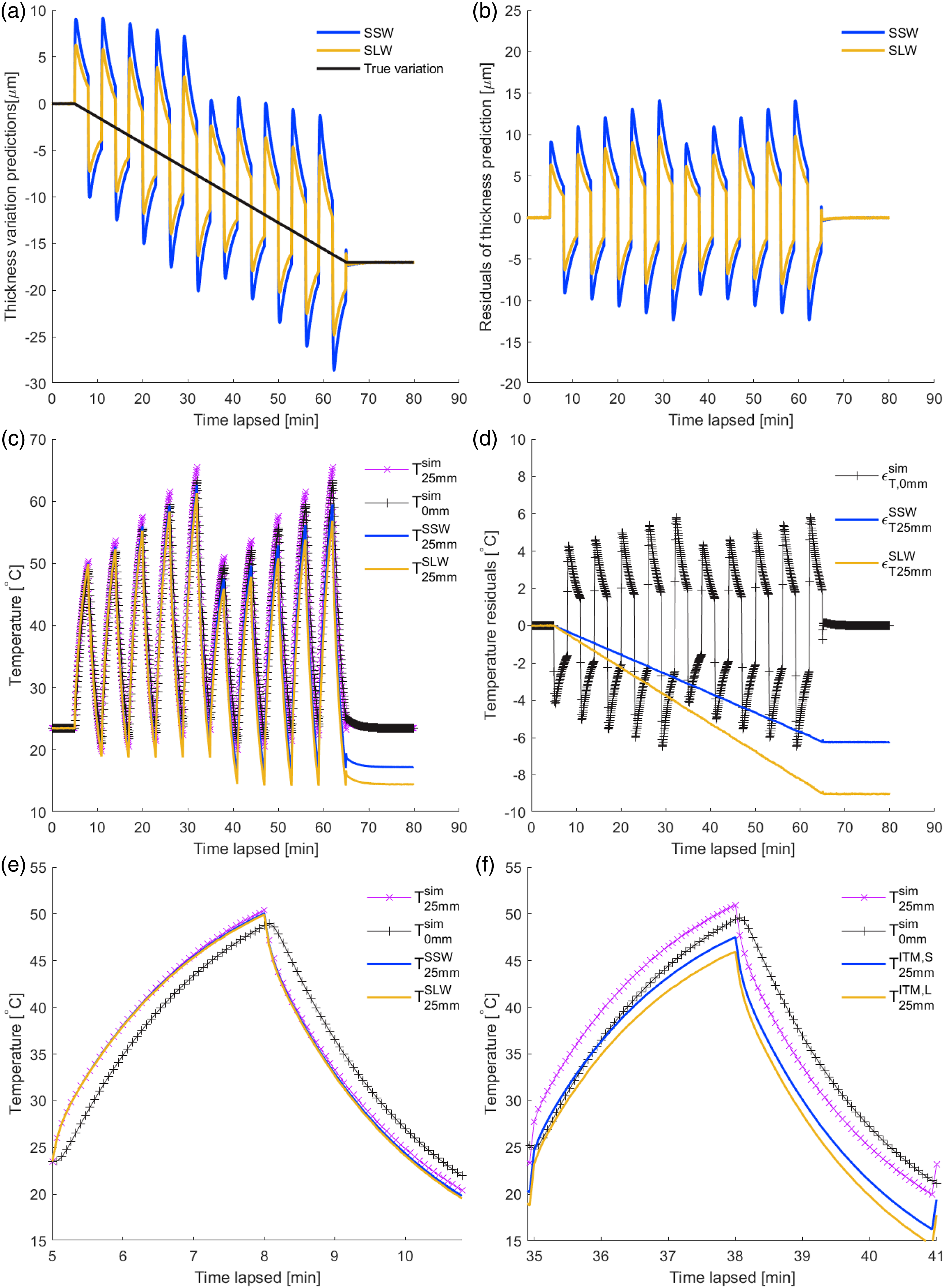

In subplot (c), ultrasonic temperature predictions are compared to the ground truth obtained from simulation. To make them directly comparable to experimental measurements, the temperature values at 25 mm, $T_{25 m m}^{s i m}$ , below Interface-A are presented in the graph. The temperature at Interface-A, $T_{0 m m}^{s i m}$ , is also shown in the graph as it is normally used for temperature monitoring if subsurface temperature predictions are unavailable. Subplot (e) and (f) present the zoomed plots of the temperature predictions around cycle-1 (5 min < t < 11 min) and cycle-6 (35 min < t < 41 min), respectively. As shown in the graphs, the ultrasonic predictions follow the true values (plotted in magenta) in Cycle-1 very closely. However, the predicted values drift away from the true values as the thickness of the system gradually reduces. In Cycle-6, or after a thickness loss of 8.5 μm (i.e. 0.028% of its nominal thickness), the ultrasonic method is seen to give even worse predictions than the one using temperature measurement at 0 mm. The gradual drift of ultrasonic predictions in the given scenario is more clearly illustrated in subplot (d), where residuals of the ultrasonic temperature predictions are shown to grow linearly with time during the period of thickness loss.

Dual-wave simultaneous prediction

Figure 7 shows the thickness and temperature predictions that can be achieved by the proposed dual-wave prediction method. The numerically generated ToF data used here is the same as was used in the previous study, Gaussian noise with standard deviation of 1 × 10⁻¹¹s is superimposed onto the noise-free ToF data and the triggering threshold for thickness correction, ϵ_T, is set to 0.1°C. In subplot (a), the trace plotted in red represents the ultrasonic thickness predictions of the dual-wave (DW) method. For comparison, the conventional SSW and SLW predictions are also plotted in blue and yellow. As shown in the graph, the dual-wave ultrasonic predictions follow the true values very closely and thickness prediction residuals as shown in the subplot (b) are below 0.5 μm throughout the period. With regards to temperature predictions, subplot (c) and (d) show that the drift seen in the previous case has been corrected with the dual-wave correction method. The maximum temperature prediction residuals are less than 0.1°C throughout the period.

Figure 7.

Comparisons between single-wave predictions and dual-wave predictions. (a) Ultrasonic thickness predictions, (b) residuals of thickness predictions, (c) ultrasonic temperature predictions and (d) residuals of temperature predictions. Blue trace: single-shear-wave prediction. Yellow trace: single-longitudinal-wave prediction. Red trace: dual-wave prediction in ideal scenario (ToF noise = 1 × 10⁻¹¹ s, ϵ_T = 0.1°C). Cyan trace: dual-wave prediction in realistic scenario (ToF noise = 5 × 10⁻¹¹ s, ϵ_T = 0.6°C).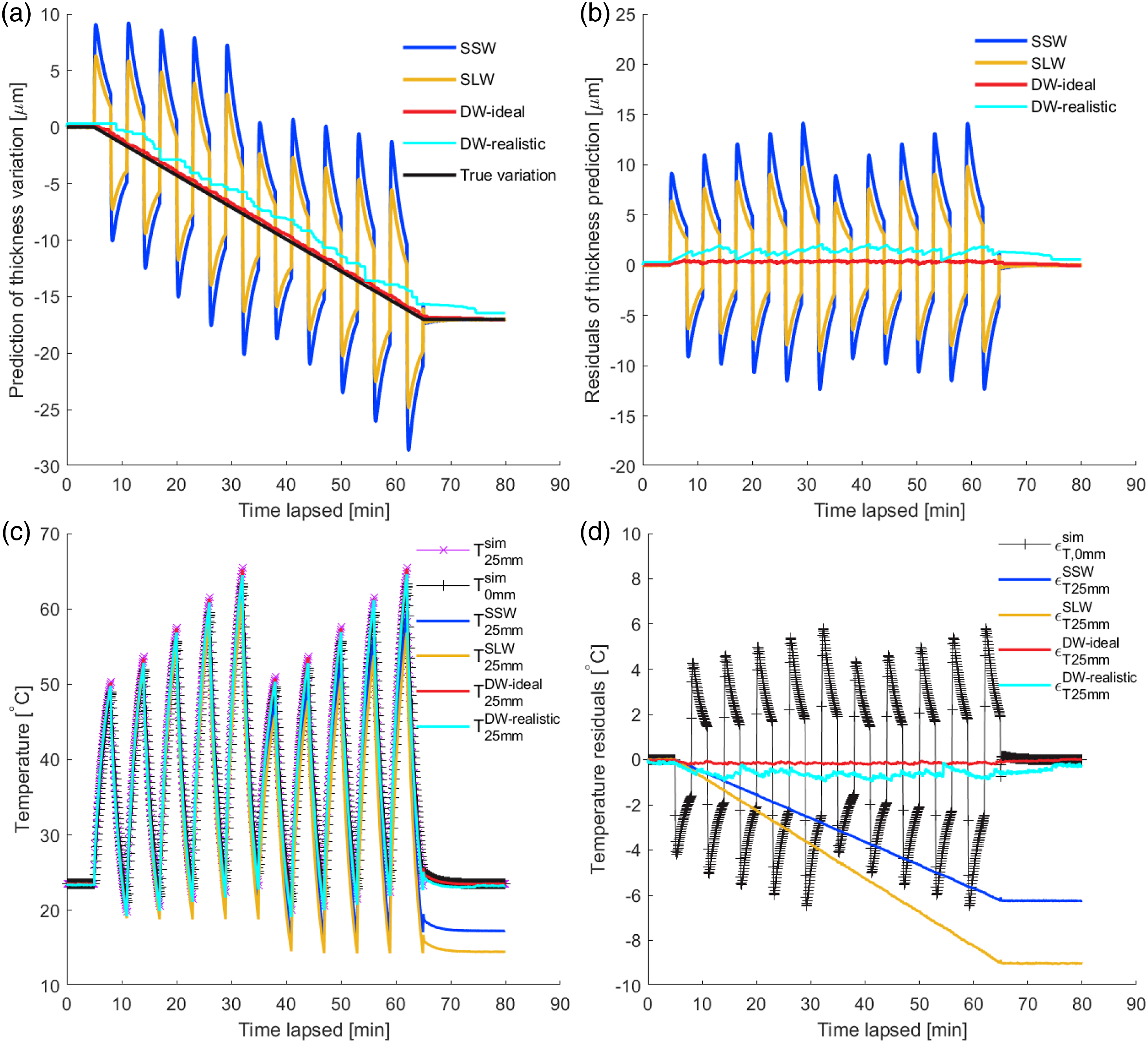

Uncertainties in time-of-flight measurement and threshold for thickness correction

Noise in the ToF measurements is an important contributor to the uncertainties of temperature and thickness predictions. To simulate a more realistic case, Gaussian ToF noise with standard deviation of 5 × 10⁻¹¹s, which is similar to what was measured in the experimental data, is superimposed onto the numerically generated ToF data. In addition, the threshold value, ϵ_T, for triggering thickness correction is also adjusted to make the algorithm less susceptible to noise and uncertainties in the input data. Unless otherwise stated, the value of ϵ_T has been set to 0.6°C in this and the following sections.

Simulation results of the more realistic case are also shown in Figure 7 as traces plotted in cyan. The increased ϵ_T value delays the onset of the thickness correction and thus results in a rightward shift of the cyan trace with multiple progressive thickness corrections. Noise in the ToF data also contributes to the ‘wobbling’ of the cyan trace but the overall effect at the given noise level is relatively small. The maximum thickness prediction residual presented in this case is around 2.1 μm compared to the uncorrected case of 15 μm. With regard to temperature predictions, the increased ϵ_T value causes a slight downward drift of the ultrasonic predictions; however, the maximum temperature deviation is still below 0.9°C.

Quantitative performance evaluation

The maximum prediction residual (max |ɛ|) and root-mean-square-deviation (RMSD) are used to quantitatively assess the performances of the dual-wave (DW) method relative to the conventional SSW and SLW predictions.

Tables 2 and 3 summarise the performance metrics in the simulated cases. In an ideal scenario with minimum ToF noise and very small temperature discrepancy threshold (σ_ToF = 1 × 10⁻¹¹s, ϵ_T = 0.1°C), the RMSD of the dual-wave thickness and temperature predictions are 0.3 μm and 0.14°C, respectively. In comparison, these values are less than a tenth of the RMSD residuals of either single-shear-wave or single-longitudinal-wave predictions.

Table 2.

Residuals of the ultrasonic thickness predictions in the simulation cases.

	σ_ToF (s)	ϵ_T (◦C)	RMSD_h (μm)			Max \|ɛ_h\| (μm)
	σ_ToF (s)	ϵ_T (◦C)	SSW	SLW	DW	SSW	SLW	DW
Ideal scenario	1 × 10⁻¹¹	0.1	6.7	4.6	0.3	14.1	9.8	0.5
Realistic scenario	5 × 10⁻¹¹	0.6	6.7	4.6	1.3	14.2	10.1	2.1

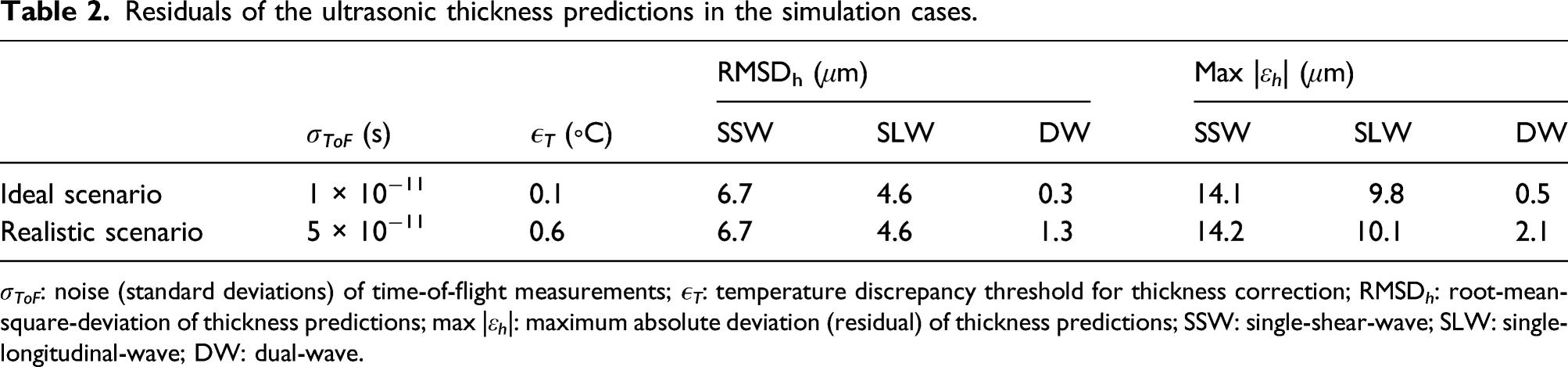
σ_ToF: noise (standard deviations) of time-of-flight measurements; ϵ_T: temperature discrepancy threshold for thickness correction; RMSD_h: root-mean-square-deviation of thickness predictions; max |ɛ_h|: maximum absolute deviation (residual) of thickness predictions; SSW: single-shear-wave; SLW: single-longitudinal-wave; DW: dual-wave.

Table 3.

Residuals of the ultrasonic temperature predictions in the simulation cases.

	σ_ToF (s)	ϵ_T (◦C)	RMSD_T (◦C)			Max \|ɛ_T\| (◦C)
	σ_ToF (s)	ϵ_T (◦C)	SSW	SLW	DW	SSW	SLW	DW
Ideal scenario	1 × 10⁻¹¹	0.1	4.1	6.0	0.1	6.3	9.1	0.3
Realistic scenario	5 × 10⁻¹¹	0.6	3.3	4.8	0.6	6.8	9.9	1.0

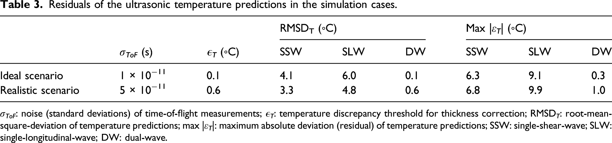
σ_ToF: noise (standard deviations) of time-of-flight measurements; ϵ_T: temperature discrepancy threshold for thickness correction; RMSD_T: root-mean-square-deviation of temperature predictions; max |ɛ_T|: maximum absolute deviation (residual) of temperature predictions; SSW: single-shear-wave; SLW: single-longitudinal-wave; DW: dual-wave.

When measurement noise and uncertainties are introduced to simulate a more realistic scenario (σ_ToF = 5 × 10⁻¹¹s, ϵ_T = 0.6°C), the RMSD of the dual-wave thickness and temperature predictions increase to 1.3μm and 0.6°C, respectively. Nevertheless, the dual-wave method still outperforms the single-wave method by approximately a factor of 5. Further realisation of the full potential of the dual-wave method can be achieved with improved ToF estimation methods and higher signal-to-noise ratio.

Experimental verification

Experimental procedures

This section describes the procedures of the experimental investigation that were conducted to verify the proposed method.

The specimen employed in the verification experiment is a cuboid mild steel (080A15/EN32B) block whose dimensions are 160 mm × 50 mm × 30 mm (L × W × T). Three holes were created on the side of the specimen at 10 mm, 20 mm and 25 mm from the Interface-A. Resistance temperature detectors (RTD) (RS PRO 2 wire PT1000 Sensor, class A, RS Components Ltd. Birchington Road, Corby, Northants, UK) were installed in the drilled holes as well as on the interface-A. The RTD temperature measurements were collected by a data log (PT-104 Platinum Resistance Data Logger, Pico Technology, St Neots, Cambridgeshire, UK). Two piezoelectric transducers were bonded to the specimen with high-temperature enduring adhesive epoxy (Duralco 4461-1, Cotronics) at approximately 8 mm apart. The transducer for generating shear ultrasonic waves is 12 mm × 1 mm × 0.25 mm in dimension and was excited by a 5-cycle hanning windowed toneburst signal with 2.4 MHz central frequency; the other transducer for generating longitudinal ultrasonic waves (PI Physik Instruments, Germany) is 10 mm in diameter and 0.5 mm in thickness and was excited by a 5-cycle hanning windowed toneburst signal with 3.2 MHz central frequency. The two excitation signals were sent to the transducers via two synchronised arbitrary function generators (AFG)/oscilloscopes (Handyscope-HS5, TiePie, Netherlands) at the same time. The reflected shear/longitudinal waves were received and converted to electrical signals by the same transducer, amplified by 40/20 dB and digitised by the AFG/oscilloscope at a sampling rate of 50 MHz.

To obtain the velocity-temperature relations of Figure 2, a calibration experiment was carried out on the specimen in a climate chamber (VCL 4003, Voetsch Industrietechnik, Weiss Technik UK Ltd, The Technology Centre, Loughborough, UK). The specimen was heated up in the chamber by air to 100°C and was maintained at the temperature for 6 h to ensure it reached an equilibrium state (uniform temperature). The air in the chamber was then slowly cooled from 100°C to 10°C at a constant rate of 0.2°C per minute. It was assumed that temperature within the specimen was uniform during the cooling phase. Ultrasonic and temperature measurements were taken every 30 s during the period. The measurements taken between 20°C and 90°C are used for the calibration.

The basic configurations of the validation experiment are presented in Figure 8. A corrosion cell is built around the specimen to create the required conditions. In this case, the temperature gradient across the specimen thickness was introduced by running hot/cold liquid through the cell, where the liquid was in direct contact with the interface-B. The liquid was 3.5% w/v NaCl solution, which was pre-prepared and stored in two separate reservoirs. Temperature of the hot liquid reservoir were regulated between 60°C and 80°C while the temperature of the cold liquid reservoir was kept between 10°C and 15°C. Thickness variation of the specimen was introduced by applying a DC current of 150 mA to initiate the galvanic forced corrosion of the specimen in a specific region.

Figure 8.

Graphical illustration of the experimental verification setup.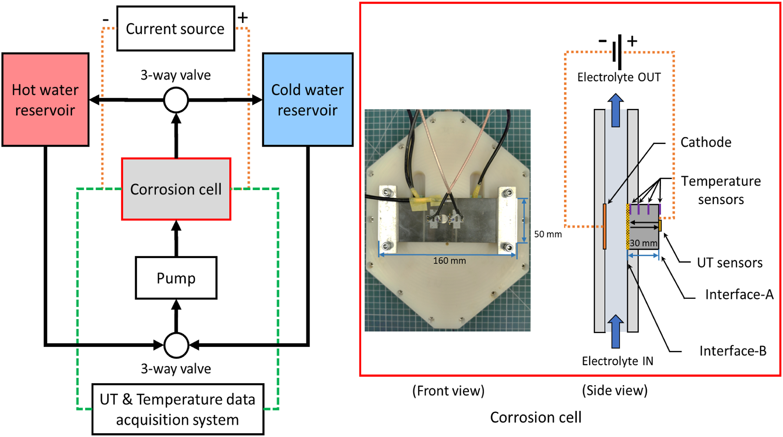

Ultrasonic thickness predictions are compared to the analytical values based on Faraday’s law of electrolysis¹⁵ and to independent optical surface profile measurements. The thickness variations predicted by Faraday’s law can be calculated by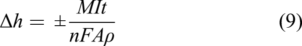

Δ h = \pm \frac{M I t}{n F A ρ}

(9)

where M = 55.5 and ρ = 7890 kg/m³ are the molar mass and density of the material, I is the applied DC current, t is the time elapsed since the start of electrolysis, n = 2 is the number of electrons lost per iron atom during its oxidation, F is Faraday’s constant and A is the area of the reaction surface.

Figure 9(a) shows the profile of the specimen surface prior to the corrosion experiment. The surface profile was stitched from six optical scans by a white-light interferometer (TMS-100 TopMap Metro. Lab, Polytec Ltd, Germany). The profile was rotated and translated in the post-processing such that the plane of the uncorroded scanned surface lies on the plane ‘Z = 0’.

Figure 9.

(a) Optical profile of the specimen surface prior to the corrosion experiment and (b) optical profile of the specimen surface post the corrosion experiment. The regions enclosed by the red dashed lines represent the reaction surfaces for electrolysis. The regions enclosed by the black dashed lines represent the reference surfaces with no corrosion.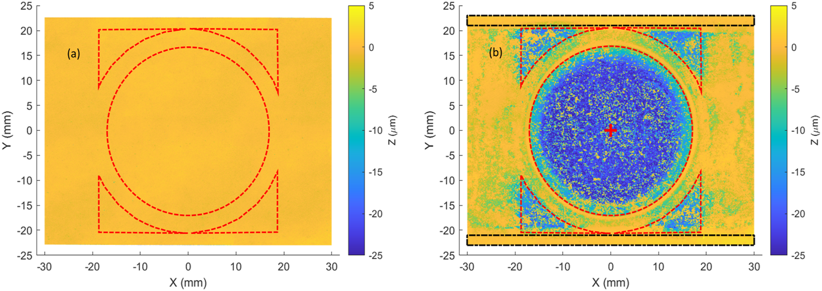

The regions enclosed by the dashed red lines are the reaction surfaces for electrolysis. These reaction surfaces were isolated from the rest of the specimen surface by a rubber ‘O-ring’ (inner diameter = 34 mm, cross-section = 3 mm) and ‘confinement walls’ such that the passing of electric current was designed to be confined between the cathode and the reaction surfaces. The combined area of reaction surfaces in this case is approximately 1160mm².

The capabilities of the proposed dual-wave correction method are presented with two case studies. In the first case, only temperature fluctuations were introduced but the thickness of the specimen remained unchanged. In the second case, both temperature and thickness of the specimen were varied.

Experimental results with temperature fluctuations only

Figure 10 shows the ultrasonic temperature and thickness measurements. Since no electrical current was applied, the thickness of the specimen remained unchanged after the thermal cycling. In subplot (a), thickness predictions given by the conventional single-wave method shows fluctuations as large as 27 μm during the period of rapid temperature changes. On the other hand, the thickness predictions using the dual-wave method are seen to only fluctuate with a maximum deviation of 3 μm. In subplot (b), ultrasonic temperature predictions at 25 mm below the exterior surface (i.e. interface-A) are compared to the RTD measurements. The residuals of ultrasonic temperature predictions (with respect to the RTD measurements) are shown in subplot (c). For comparison purpose, the differences between RTD measurement at 0 mm and 25 mm are overlaid in the same plot. As can be observed from the graphs, ultrasonic temperature predictions in general follow closely with the RTD measurements. However, residuals of the ultrasonic predictions show ‘transient’ spikes at the transitions between heating and cooling. Nevertheless, the residuals remain below ±2°C during most of the period. In addition, as explained in our previous study,¹³ RTD temperature measurements tend to trail/lag behind the ultrasonic predictions and this phenomenon can cause the observed spikes in residuals. To illustrate this lagging effect, in subplot (d) the reference RTD temperature measurements $(T_{25 m m}^{R T D})$ are shifted forward by 4 s (i.e. one measurement interval, $T_{25 mm}^{RTD} |_{t = m} = T_{25 mm}^{RTD} |_{t = m + 1}$ , where m denotes an arbitrary index in time). As shown in the graph, after the temporal shift the spikes at the heating/cooling transitions are greatly suppressed.

Figure 10.

Experimental results with temperature fluctuations only. (a) Ultrasonic thickness predictions, (b) ultrasonic temperature predictions at 25 mm depth with the dual-wave simultaneous corrections applied, (c) residuals of the ultrasonic temperature predictions (with respect to resistance temperature detectors measurements) and (d) additional ‘simulated’ case, where the reference temperature measurements 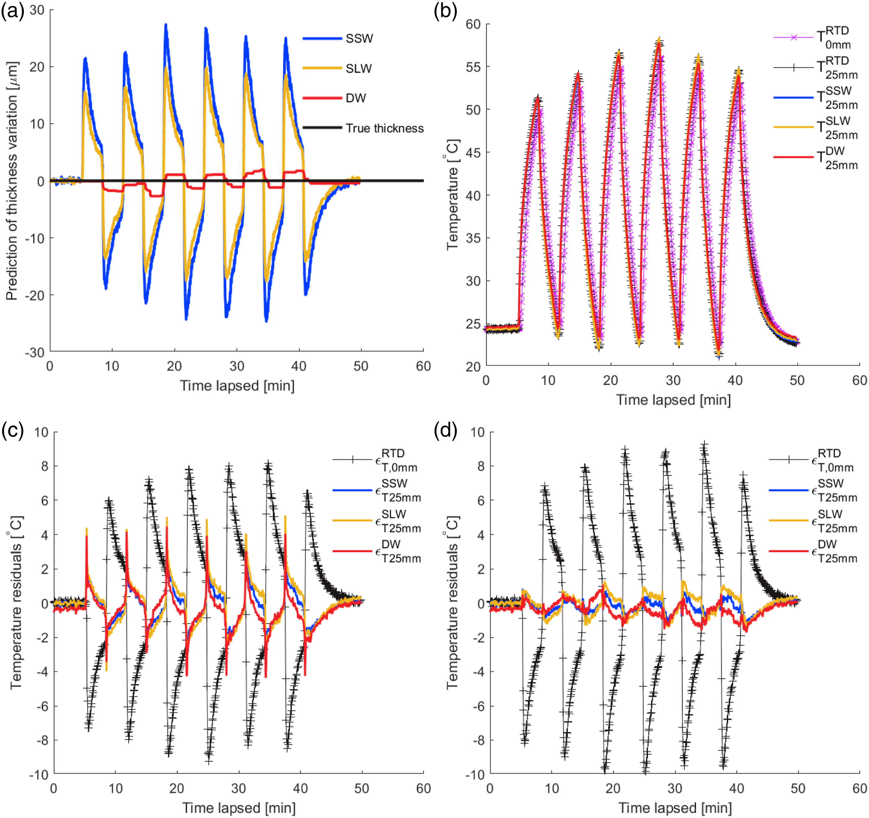$T_{25 m m}^{R T D}$ are brought forward by one measurement interval (i.e. 4 s). Blue trace: single-shear-wave prediction. Yellow trace: single-longitudinal-wave prediction. Red trace: dual-wave prediction.

Experimental results with both temperature fluctuations and corrosion

The second experiment was performed immediately after the first one and a DC current of 150 mA was applied to introduce thickness reduction of the specimen. Subplot (a) and (b) of Figure 11 demonstrate the thickness tracking capability of the dual-wave method when both temperature and thickness vary simultaneously. For the conventional single-wave method, thickness measurements fluctuate around the values predicted by Faraday’s law. Maximum measurement residuals are around 20 μm for the shear wave and 15 μm for the longitudinal wave. In comparison, the dual-wave predictions follow the predictions using Faraday’s Law more closely. The maximum deviation of the dual-wave predictions is less than 4 μm. However, it is worth noting that there seems to be a gradual buildup of the residuals. At the end of the experiment, Faraday’s law predicts a thickness reduction of 17.0 μm while the dual-wave method predicts 15.0 μm. At the same time, thickness loss predicted by single shear and longitudinal waves are 17.8 μm and 16.8 μm, respectively.

Figure 11.

Experimental results with both temperature fluctuations and corrosion. (a) Ultrasonic thickness predictions. The error bar of the optical measurement shows a confidence range with 99.7% probability (3σ) based on the technical specifications of the interferometer,¹⁶ (b) residuals of the thickness predictions, (c) ultrasonic temperature predictions at 25 mm depth and (d) residuals of the ultrasonic temperature predictions (with respect to resistance temperature detectors measurements). Blue trace: single-shear-wave prediction. Yellow trace: single-longitudinal-wave prediction. Red trace: dual-wave prediction.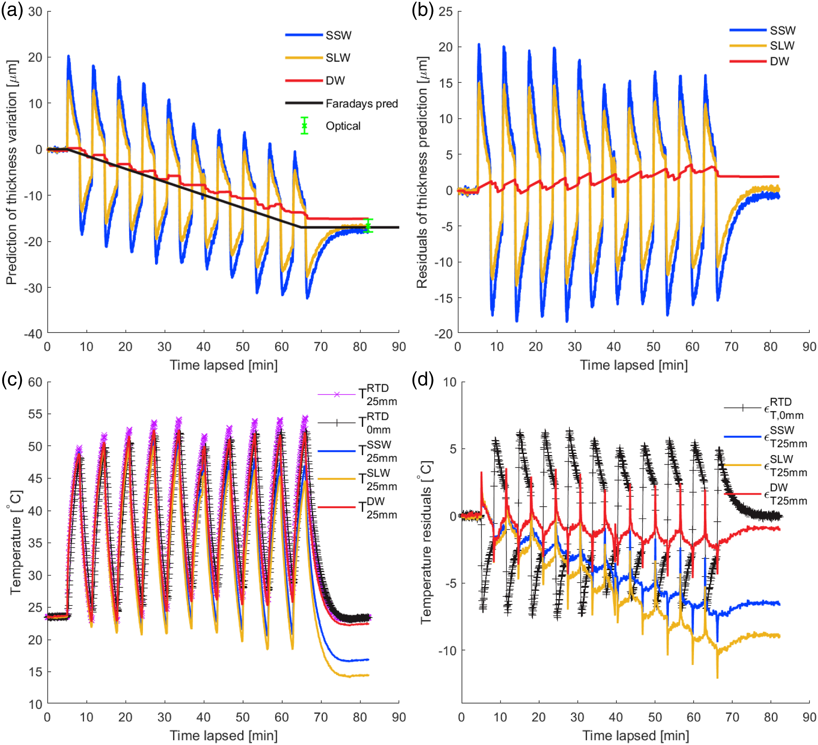

Figure 9(b) presents the surface profile of the specimen after the experiment. Corrosion patches can be clearly observed in the reaction surface enclosed by the dashed red lines. Other regions on the surface between −21 mm < Y < 21 mm show some slight traces of corrosion due to leakages from the ‘confinement’ structures. The areas enclosed by the black dashed lines are sealed by a silicon gasket sheet and therefore show little sign of corrosion. These regions are used as the reference plane to calculate the corrosion depth. The independent optical measurements taken by the white-light interferometer show a mean thickness reduction of −16.6 ± 1.4 μm.

Subplots (c) to (f) of Figure 11 compare the ultrasonic temperature predictions with and without the dual-wave correction being applied. Similar to what has been shown in the simulation, without taking the thickness loss into account, SSW and SLW temperature predictions (the blue and yellow traces) drift over time with increasing thickness loss. The accumulated prediction residuals at the end of the experiment reached −6.5°C and −8.9°C for SSW and SLW predictions, respectively. On the other hand, when the DW method is applied (the red trace), about 90% of the drifting were corrected and the accumulated prediction residuals are limited to −1°C by the end of the experiment.

Tables 4 and 5 summarise the performance metrics in the corroding and non-corroding experiments. In the case without thickness variations, the RMSD of DW thickness predictions (1.2 μm) is close to a tenth of that of the SSW (12.6 μm) and SLW (9.2 μm) thickness predictions. On the other hand, the RSMD of DW temperature predictions (1.1°C) are very close to that of the SSW (1.0°C) and SLW (1.3°C) temperature predictions. In the case where both temperature and thickness of the specimen varied at the same time (the corroding case), the DW method reduces the RMSD of thickness predictions from 10.0 μm/7.3 μm (SSW/SLW) to 1.7 μm (DW). In addition, the dual-wave method also reduces the RMSD of temperature predictions from 4.8°C/6.4°C (SSW/SLW) to 1.5°C (DW).

Table 4.

Residuals of ultrasonic thickness predictions in the verification experiments.

Experimental case	RMSD_h (μm)			Max \|ɛ_h\| (μm)
Experimental case	SSW	SLW	DW	SSW	SLW	DW
With temperature fluctuation only	12.6	9.2	1.2	27.3	19.8	2.7
With both temperature fluctuations and corrosion	10.0	7.3	1.7	20.4	15.0	3.6

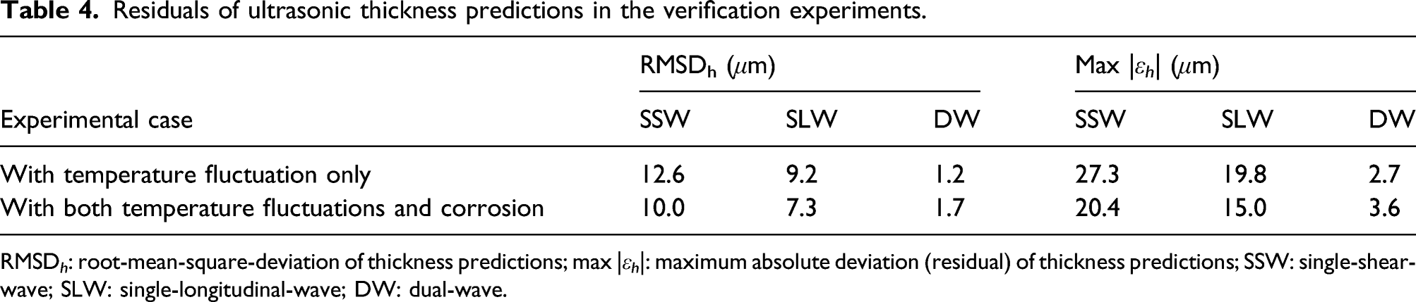
RMSD_h: root-mean-square-deviation of thickness predictions; max |ɛ_h|: maximum absolute deviation (residual) of thickness predictions; SSW: single-shear-wave; SLW: single-longitudinal-wave; DW: dual-wave.

Table 5.

Residuals of ultrasonic temperature predictions in the verification experiments.

Experimental case	RMSD_T (◦C)			Max \|ɛ_T\| (◦C)
Experimental case	SSW	SLW	DW	SSW	SLW	DW
With temperature fluctuation only	1.0	1.3	1.1	4.5	5.1	4.5
With both temperature fluctuations and corrosion	4.8	6.4	1.4	9.4	12.1	4.6

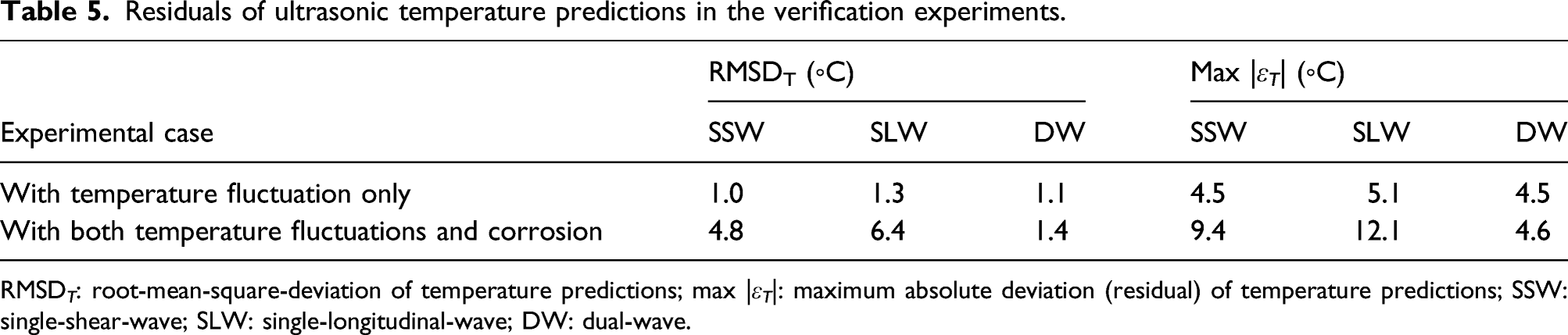
RMSD_T: root-mean-square-deviation of temperature predictions; max |ɛ_T|: maximum absolute deviation (residual) of temperature predictions; SSW: single-shear-wave; SLW: single-longitudinal-wave; DW: dual-wave.

To summarise, the dual-wave prediction method has shown substantial improvements relative to the conventional single-wave methods under the same conditions. The benefits offered by the dual-wave method will be positively correlated with increasing specimen thickness, increasing magnitude of thermal stimuli and reducing thermal conductivity of the material.

Discussion on non-uniform thickness change

The potential sources of the gradual increase in prediction residuals shown in Figure 11 were also investigated. The dual-wave correction algorithm assumes that the areas being monitored by the shear and longitudinal waves undergo exactly the same thickness reduction. However, the corrosion patch generated by electrolysis was not perfectly uniform and the piezoelectric transducers, despite being positioned in close proximity to each other, might be sensing slightly different thickness changes during the experiment. This can be observed in the graphs of Figure 11, where the final thickness measurements of the single shear and longitudinal waves are −17.8 μm and −16.8 μm, respectively.

Two additional simulations were performed to verify that non-uniform thickness changes could cause the observed drift in ultrasonic predictions. In the first case, the rates of thickness change were set to −17.8 μm/hr and −16.8 μm/hr for the shear and longitudinal waves while the two values were swapped in the second case.

Figure 12(a) and (b) present the ultrasonic thickness predictions where the actual rate of thickness reduction of the shear wave exceeds that of the longitudinal wave. In this case, the dual-wave method predicts a thickness loss of −14.9 μm, which is smaller than the nominal value and any of the single-wave predictions. This resembles with what has been observed in Figure 11. Figures 12(c) and (d) present the opposite case, where the actual thickness change for the longitudinal wave exceeds that for the shear wave. In this case, the dual-wave predictions first lag behind the nominal values due to the delayed onset of thickness correction, however, as time lapses the dual-wave method predict a higher rate of thickness loss. At the end of the simulated case, the final thickness change predicted by the dual-wave method reaches around −19.5 μm.

Figure 12.

Ultrasonic predictions with non-uniform corrosion depth. (a) and (b): Ultrasonic thickness predictions and prediction residuals for the case Δh_nominal = −17.0 μm, Δh_S = −17.8 μm, Δh_L = −16.8 μm. ToF noise = 5 × 10⁻¹¹ s, ϵ_T = 0.4°C. (c) and (d): Ultrasonic thickness predictions and prediction residuals for the case Δh_nominal = −17.0 μm, Δh_S = −16.8 μm, Δh_L = −17.8 μm. ToF noise = 5 × 10⁻¹¹ s, ϵ_T = 0.6°C. Blue trace: single-shear-wave prediction. Yellow trace: single-longitudinal-wave prediction. Red trace: dual-wave prediction.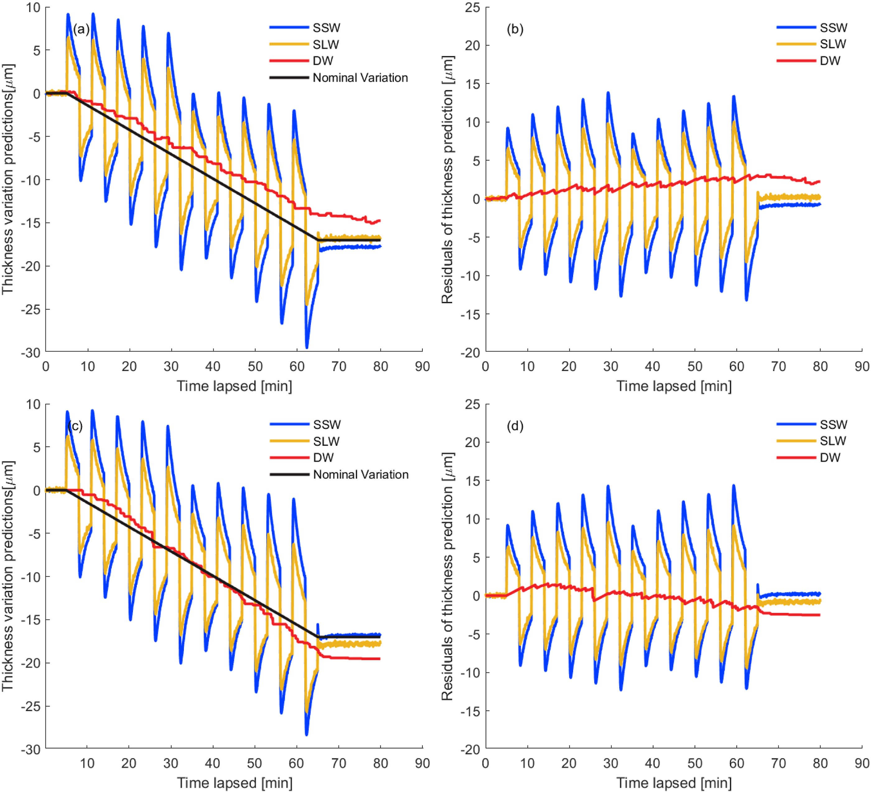

To summarise, Figure 12 demonstrates that the observed drift in ultrasonic predictions can be explained by the increasing spatial non-uniformity of the thickness loss over the reaction areas. Further research is in progress to understand the robustness of the dual-wave method to different measurement uncertainties. The design and configuration of the ultrasonic transduction systems can also be improved such that the shear and longitudinal waves being excited in the specimen are truly ‘co-located’ (i.e. being excited at the same location and with similar aperture and energy beam spread).

Conclusion

In this study, we propose a dual-wave (i.e. shear and longitudinal ultrasonic waves) approach to simultaneously monitor thickness loss and through-thickness temperature distributions of a plate-like structure. We showed that the method can differentiate between ToF changes due to thickness variation and temperature fluctuation under the given conditions. Hence, the proposed dual-wave prediction method has addressed a key inherent limitation of the conventional ultrasonic temperature sensing techniques, and can further improve the performances of conventional thickness gauging methods under complex environmental conditions.

The results of verification experiments showed that the proposed dual-wave correction method can substantially reduce drift in temperature predictions due to gradual thickness loss. The accumulated temperature prediction residuals were reduced from 8.9°C to less than 1°C, or by a factor of 9. The RMSD of temperature predictions was also reduced from 6.4°C to 1.4°C.

From the perspective of thickness gauging, the proposed method reduced prediction fluctuations due to subsurface temperature gradients by approximately a factor of 5. The RMSD of thickness prediction was reduced from 10 μm to 1.7 μm while the maximum prediction residual was reduced from over 20 μm to 3.6 μm. Further improvements may be realised with improved signal-to-noise ratio and ToF measurement repeatability.

Spatially non-uniform thickness variations were shown to adversely affect the performances of the proposed dual-wave prediction method. Optimisation of the algorithm is possible and purpose-built ultrasonic transduction systems may be developed to alleviate the adverse effects. Further research needs to be carried out to assess the performances of the method under industrial conditions in field trials.

Footnotes

Acknowledgements

The authors would like to thank the anonymous reviewer for the many useful suggestions to improve this manuscript, in particular the discussion around Equations (6) and () which highlights the effect of thickness changes on ultrasonic temperature predictions.

Declaration of conflicting interests

The author(s) declared no potential conflicts of interest with respect to the research, authorship, and/or publication of this article.

Funding

The author(s) received no financial support for the research, authorship, and/or publication of this article.

ORCID iD

Yifeng Zhang

References

Mariani

Heinlein

Cawley

. Compensation for temperature-dependent phase and velocity of guided wave signals in baseline subtraction for structural health monitoring. Struct Health Monit 2019; 19: 26–47. DOI: 10.1177/1475921719835155

Yue

Aliabadi

. A scalable data-driven approach to temperature baseline reconstruction for guided wave structural health monitoring of anisotropic carbon-fibre-reinforced polymer structures. Struct Health Monit 2019; 19: 1487–1506. DOI: 10.1177/1475921719887109

Rommetveit

Johansen

Johnsen

. A combined approach for high-resolution corrosion monitoring and temperature compensation using ultrasound. IEEE Trans Instrum Meas 2010; 59(11): 2843–2853. DOI: 10.1109/TIM.2010.2046598

Adamowski

Buiochi

Tsuzuki

et al. Ultrasonic measurement of micrometric wall-thickness loss due to corrosion inside pipes. In: IEEE International Ultrasonics Symposium, IUS, Prague, Czech Republic, 21–25 July 2013, pp. 1881–1884. DOI:10.1109/ULTSYM.2013.0479

Zou

Cegla

. High accuracy ultrasonic monitoring of electrochemical processes. Electrochem Commun 2017; 82: 134–138. DOI: 10.1016/j.elecom.2017.07.020

Cheong

Kim

. High-temperature ultrasonic thickness monitoring for pipe thinning in a flow-accelerated corrosion proof test facility. Nucl Eng Technol 2017; 49(7): 1463–1471. DOI: 10.1016/j.net.2017.05.002

Cheong

Kim

, et al. On-line monitoring of pipe wall thinning by a high temperature ultrasonic waveguide system at the flow accelerated corrosion proof facility. Sensors 2019; 19(8): 1762. DOI: 10.3390/s19081762

Ihara

Takahashi

. Ultrasound thermometry for monitoring internal temperature gradient in heated material. In: Proceedings - IEEE Ultrasonics Symposium 2009, Rome, Italy, 20–23 September 2009, pp. 1199–1202. DOI:10.1109/ULTSYM.2009.5441882

Gajdacsi

Jarvis

Huthwaite

, et al. Reconstruction of temperature distribution in a steel block using an ultrasonic sensor array. J Nondestruct Eval 2014; 33(3): 458–470. DOI: 10.1007/s10921-014-0241-0

10.

Jia

Chernyshev

Skliar

. Ultrasound measurements of segmental temperature distribution in solids: method and its high-temperature validation. Ultrasonics 2016; 66: 91–102. DOI: 10.1016/j.ultras.2015.11.006

11.

Wei

Shi

, et al. Reconstruction of internal non-uniform temperature distributions in solid structures. J Eng Thermophys 2016; 37(5): 1055–1060 (in Chinese).

12.

Wei

You-An

Bi-Nan

, et al. Reconstruction of internal temperature distributions in heat materials by ultrasonic measurements. Appl Therm Eng 2017; 112: 38–44. DOI: 10.1016/j.applthermaleng.2016.09.169

13.

Zhang