
Abstract
A significant problem associated with the implementation of Vibration-Based Structural Health Monitoring (VSHM) systems originates from the detrimental effects caused by Environmental and Operational Variations (EOVs). The EOVs cause observations from the same structural condition to behave in different manners. As such, this leads to issues when defining a robust baseline state as well as making the discrimination between undamaged and damaged observations more challenging. In order to address these challenges, multivariate nonlinear regression is implemented to account for the EOVs. Damage Sensitive Features (DSFs) are extracted from acceleration data and then are regressed based on environmental and operational parameters. New features are effectively normalised by finding the difference between the measured and predicted values. This process removes the influence of the EOVs in an explicit manner, allowing for more reliable damage detection. While the benefit of the application of different regression methodologies has already been demonstrated in the past, this work addresses a number of practicalities in the implementation of VSHM on real systems. The analysis investigates the selection of the DSF and is investigated alongside another analysis into how the damage detection behaves under varying amounts of input information. Furthermore, a method is proposed to understand and account for a large number of outliers in the training data.
Keywords
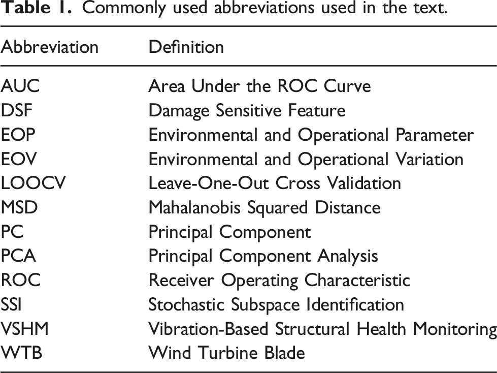
Abbreviations
Commonly used abbreviations used in the text.
Introduction
As wind turbines continue to increase in size, 1 the problem of maintaining them becomes a larger and more complex issue. The industry standard for maintaining the blades is mostly done through visual inspection, whether it is by an engineer abseiling down the blades or through images captured via drones or other devices. 2 Not only are these methods dangerous, especially when considering an engineer inspecting an offshore wind turbine, and expensive, they are also sparse. 3 When impacted, Wind Turbine Blades (WTBs) become susceptible to delamination and cracking which needs to be monitored so that the damage does not degenerate further. As such, there is a real need for a maintenance system that can work in real time, online and in remote locations. 4
A method that can be implemented to resolve these problems is Vibration-Based Structural Health Monitoring (VSHM). VSHM can be broken into two main types; model-based and data-driven. As the name suggests, model-based methods rely on physical or computer based models, such as a finite element model. These methods, typically used in the earlier stages of VSHM, tend to be more interpretable as they are based on physical laws but can also be time consuming to create and to operate. 5 Data-driven methods use only measurements taken from the structure and often do not consider any physics. However, the Damage Sensitive Features (DSFs) can often integrate aspects of physical laws or properties such as natural frequencies. These methods are usually computationally less expensive but need to be carefully designed so that they function appropriately. 6 This work is focused on the data-driven approach.
A significant issue that challenges VSHM is the presence of Environmental and Operational Variations (EOVs). Many research studies have shown that the presence of EOVs can reduce the overall damage detection capabilities by masking its effects.7,8 For example, temperature has been shown to have a larger effect on the dynamics of a structure than small amounts of damage. 9 The problem associated with the EOVs can be further exacerbated when studying offshore structures since they experience more extreme conditions. 10 As such, an ideal VSHM method can remove the influence of the EOVs without discarding information about the damage. 11
The aforementioned problem can be attempted in two different ways, implicitly and explicitly. In an implicit method, information about the Environmental and Operational Parameters (EOPs) are not given to the system and, thus, they require less data. A popular method of this type is Principal Component Analysis (PCA).12–14 PCA is a linear transformation method used in VSHM, which attempts at finding orthogonal vectors pointing at the directions of maximum variation in the data. In its application in VSHM, components with the largest variance are assumed to be heavily influenced by EOVs and are discarded.15,16 The downside of this is that the potential influence of the damage might also be removed. Cointegration is another example of an implicit method that has been implemented to remove the influence of EOVs.17,18 The latter attempts at removing common trends in the DSFs by considering their temporal structure.
In an explicit method, EOPs are given directly to the system with the aim of capturing their joint effect on the DSFs. 19 The aim of these methods is to normalise the DSFs by modelling them as a function of the EOPs. 20 This problem is solved by different types of regression. A downside to this method is that the EOPs that heavily influence the system are not always easy or feasible to measure. However, the results obtained are often more interpretable. Thus, a better understanding of how the EOPs affect the system is gained. Additionally, explicit methods could provide additional stability by gaining a deeper understanding of the cause-effect relationship between the EOPs and the DSFs as well as being able to determine benign outliers.
The most basic form of regression that can be used for an explicit method is linear regression. Peeters and De Roeck 21 applied linear regression to data taken from the experimental Z24 bridge in Switzerland. 21 They aimed to filter out the temperature effects that were present in the natural frequencies of the bridge. In the same work, multiple environmental and operational inputs were also tested but did not yield a substantial improvement in contrast to the case of using only temperature. In order to detect damage, the residual between the prediction from the regression model and the measured value was analysed. It was found that once damage was present, there was a shift in the value of this residual. Another important point that was raised was that when compared to the work of Sohn et al., the data normalisation procedure is problem-specific and should change depending on the structure being analysed.8,22
In the work by Peeters and De Roeck, 21 the behaviour of the natural frequencies was considered to comply with a bilinear model. 21 However, Wah et al. found that the natural frequencies of the Z24 bridge could also be modelled in a nonlinear manner. 23 This work took a different approach where the natural frequencies were modelled using other natural frequencies as predictors, rather than the temperature. They found that by using the natural frequencies as both dependent and independent variables, they were able to provide better damage detection when compared to traditional regression models. As with linear regression, nonlinear regression can also be applied with multiple input variables. The paper by Roberts et al. modelled frequency transformation based features using multiple EOPs taken from an operational wind turbine. 19 It was found that the features corrected by regression models outperformed those from a PCA-based implicit method.
The linear and nonlinear approaches are both examples of deterministic approaches. However, it is also possible to apply stochastic methods in the context of structural health monitoring. Avendaño-Valencia and Chatzi 24 implemented a Gaussian Process Regression Vector AR method on data extracted from a simulated WTB. 24 The vibration responses were modelled based on uncertain inputs. They showed that this is a more robust method for damage detection since the proposed method was still able to detect damage under uncertainty. Avendaño-Valencia et al. then applied a similar Gaussian Process Regression method to data taken from an operational WTB. 20 This work showed the potential of a stochastic framework on real data in the context of structural health monitoring.
The method proposed in this work is focused around a multivariate nonlinear regression, where DSFs are modelled on the basis of multiple available EOPs. The premise of this is to show that by removing the influence of the EOPs from the DSFs, the information on damage is retained and accentuated. While different types of regression have been demonstrated in the past, the practical application is not straightforward, but involves several considerations.22,25–27 Firstly, when multiple EOPs are available, it is necessary to recognise which are influential and which are irrelevant or even detrimental. 28 A similar analysis can be made for multiple DSFs. In addition, DSFs, being estimated quantities, tend to be affected by noise and outliers, which have a considerable effect in the regression performance. Outliers in regression can lead to bias in the models which then subsequently affect estimates. 29 Poorer quality of estimates will then lead to an undesirable increase in the number of false positives and false negatives within the SHM system.
Accordingly, the main aim of the present work is to formally address these practicalities related to the construction of robust regression models for compensation of EOVs in VSHM, with the application of damage detection in WTBs. In particular, the problem of outliers in DSFs is considered and addressed by defining a method for predicting when those outliers will become false alarms in the damage detection thus alleviating the bias which they create within the regression models. Furthermore, damage detection performance under various combinations of DSFs is investigated. Gradually, increasing amounts of information from each sensor was given to the regression model and the damage detection performance was evaluated. In parallel, a discussion is used to highlight a number of relevant issues associated with the application of multivariate nonlinear regression. These include reducing data dimension, overfitting of model orders and including EOPs which bear no influence on the DSFs.
To evaluate the method in this work, two different case studies are analysed. The first comprises of the simulated vibrations of a wind turbine undergoing typical EOV patterns. The blade is also simulated under extreme weather conditions before damage is introduced. The challenge here is to recognise when there is actual damage or an extreme environmental condition. Following this, the data taken from an operational Vestas V27 wind turbine blade is considered. In this monitoring campaign, damage is incrementally introduced in the form of a crack along the trailing edge of the blade. 13 The method and results for both case studies are visually represented to show how the method is applied and the improvement in contrast to a traditional PCA-based method.
The remainder of the paper is laid out as follows. Firstly, the overall methodology is presented, which includes the multivariate nonlinear regression, model optimisation and outlier analysis. Following this, the simulated case study is presented along with a description and results. Next, the description and results for the real WTB are presented. An additional discussion used to investigate the practicalities of the implementation of this type of system. Finally, conclusions will be drawn to compose an overall evaluation of the methodology.
Methodology
This section will outline first the specific regression modelling technique that is used, including how the models are optimised. Subsequently, the method used for novelty detection is described.
Multivariate Nonlinear Regression
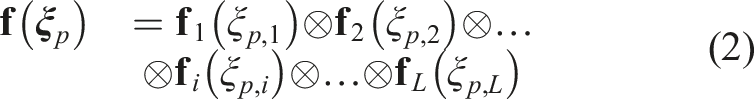
When information is available for the environmental and operational conditions, multivariate nonlinear regression can be used to model the DSFs (
The overall training multivariate functional basis can be represented by 
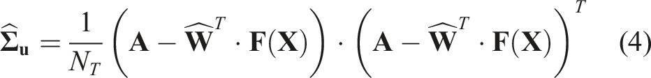
Once the coefficient matrix has been determined, an estimate for each feature across all observations can be calculated from equation (1). The final step is to extract the corrected features, 
Model Optimisation
To ensure that the features are well represented by the multivariate nonlinear regression models, a Leave-One-Out Cross Validation (LOOCV) method is used. A cross validation procedure is implemented because it gives a good estimate on how well the models are going to predict information that is not included in the training phase. The multivariate nonlinear regression models are constructed using the training data for every possibility of excluding one observation. 30 For example, if a training data set contained 100 observations, then a total 100 possibilities of missing one observation would be tested. The cumulative error of the cross validation observations is used as an estimate of the generalisation error of the nonlinear regression model. The expected outcome is that the training error will continue to reduce with increasing model order, whereas the validation error will decrease and then increase again as the model starts to overfit.
In this work, the cumulative cross validation error was calculated for every combination of input variables with orders 1–5. Since five input variables are used, a total of 3125 combinations were tested for each feature within the feature vector. Models with higher orders could be tested but this would become computationally expensive for long feature vectors. The model for each feature was chosen based on which combination had the lowest cumulative cross validation error.
Outlier Analysis
For a system to have the ability to distinguish between undamaged and damaged observations a novelty index is used, which for this study is the Mahalanobis Squared Distance (MSD). This damage index has been used in many previous works.13,14 The equation for the MSD is given below
Damage diagnosis is based on the calculated MSD and a predefined threshold value μ. The threshold is defined to be the point where 98% of the training data is accounted for according to a Chi-Square distribution with the number of degrees of freedom equal to the length of 

Case Studies
In this section, a total of two case studies will be explored to demonstrate the capabilities of the proposed methodology. The first case will be a simpler computational model of a WTB and the second will be a more complex example using data taken from an operational Vestas V27 WTB.
Simulated Wind Turbine Blade
System Description
The simulated system is based on a 40m long blade with a NACA 64–618 airfoil profile. For the simulation, the blade was modelled as an 8 degree-of-freedom aeroelastic system in a cantilever arrangement as shown in Figure 1(a). The beam was modelled using Euler–Bernoulli elements with proportional damping in such a way that the rotational dynamics can be ignored.
31
The blade was subjected to a varying temperature and wind speed, shown in Figure 1(b) and Figure 1(c), respectively, in order to emulate real conditions. The temperatures and wind speeds used in the simulation are based on average values in north-central Switzerland. This information was provided by the Federal Office of Meteorology and Climatology and The Swiss Wind Power Data Website, respectively. Further information on the simulation can be found in the original article.
24
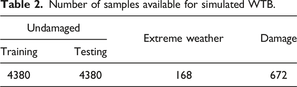
Reference figures for simulated WTB. (a) Representative cantilever beam made of Euler-Bernoulli elements with rotation and deflection degrees of freedom, (b) temperature experienced for each observation and (c) wind speed for each observation.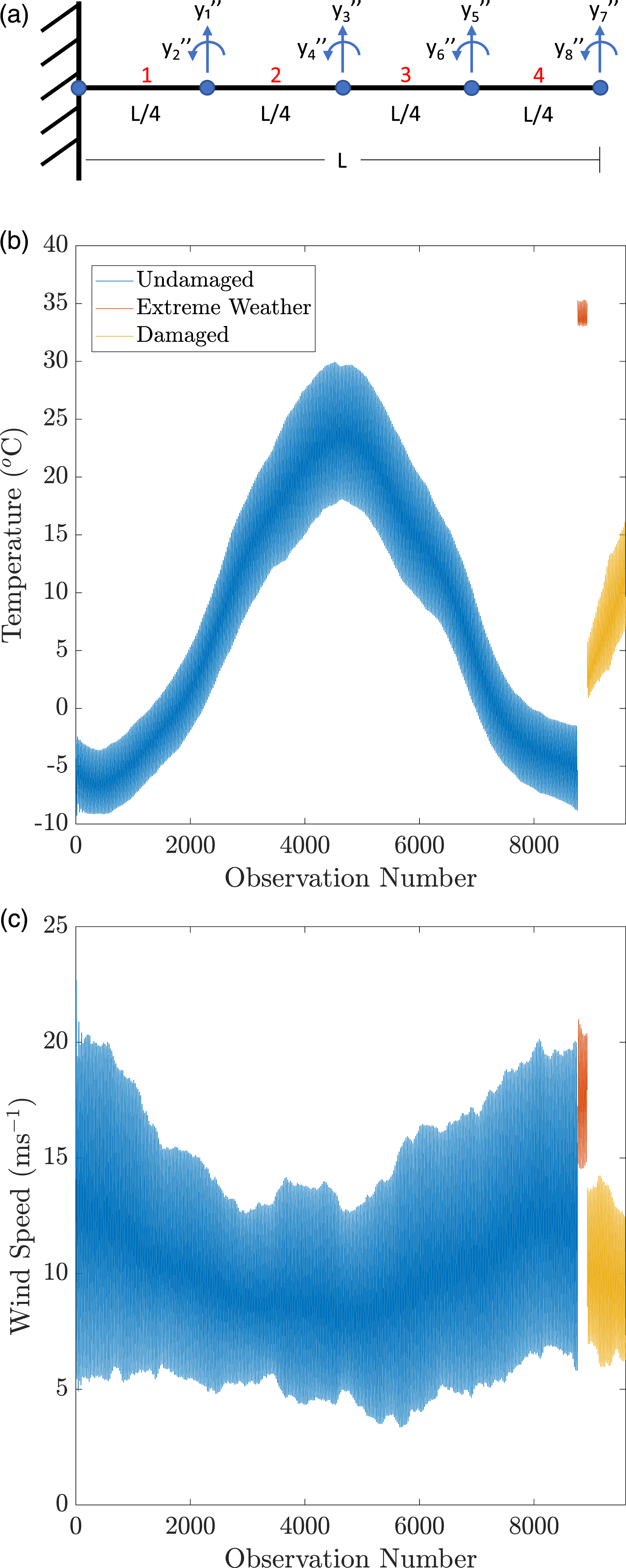
Number of samples available for simulated WTB.
Feature extraction
The DSFs that were used in this case study were the natural frequencies of the system. The natural frequencies were extracted from the raw acceleration data using Stochastic Subspace Identification (SSI), specifically the output covariance approach. The SSI methodology works in three main stages; data preprocessing, system identification and post-processing or modal analysis. In the modal analysis stage, the modal parameters are determined based on the output stabilisation diagram. The DSF that is used for damage identification, for each observation, is a single vector containing the first six natural frequencies such that
System Analysis
To study the capabilities of the multivariate nonlinear regression, the features themselves must be studied to show whether they are suitable for regression models. The natural frequency features were used in this case study since they are easily detected at lower frequencies as well as being more intuitive for illustrative purposes. The sampling frequency in the simulation was 40 Hz, which corresponds to the range of structural resonances. The first six natural frequencies from the system were used since they were stable and non-overlapping. It can be seen from Figure 2 that when each of the natural frequencies are compared to the temperature, there is a clear dependency. Specifically, it is important to consider the relationship between the undamaged observations and the temperature since these are the observations that the regression models are constructed with. As with previous work, the higher natural frequencies experience a larger range of values from the changing temperature than the lower ones.
33
Trend of natural frequencies from simulated WTB against temperature for natural frequencies (a)–(f) α1 − α6. Each figure shows the natural frequencies for the undamaged, extreme weather and damaged conditions.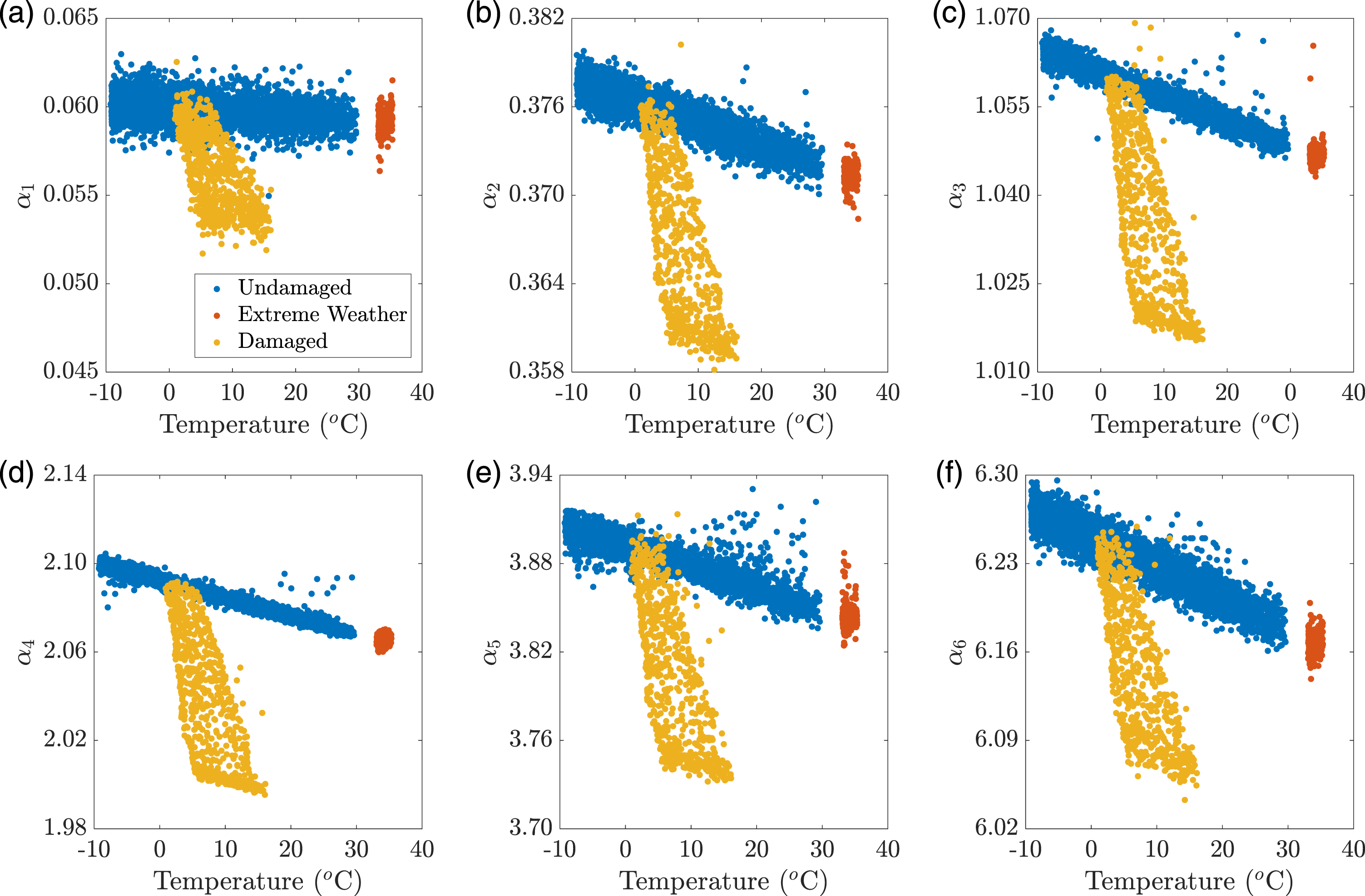
As such, a regression model can be created to model the DSFs based on the temperature and the wind speed, the only two EOPs affecting the system. A separate model was created, using the training data, for each natural frequency. Optimisation of the model order was viable on each feature, since there were a relatively small number of features. Using the LOOCV method, the order of the model which best fitted the data was chosen, with each variable tested with orders 1–5 as described in the methodology. From a visual inspection of Figure 2, the natural frequencies appear to have a linear relationship with temperature, this finding was reflected in the optimised orders. Using the defined regression models, values for the features were estimated for all of the damage scenarios including the training data. As mentioned in the methodology, the corrected features were found by taking the difference between the measured and estimated values.
Using the defined outlier analysis, a comparison can be made on the damage detection performance of the original natural frequencies against the regression corrected values. Figure 3 shows the control charts for the two different feature sets. On an initial inspection, the regression corrected features perform on a similar level of damage detection to the original features. Notably, the overall performances of the system before and after the correction are very good. Both systems have a large overlap across the testing and training as well as being able to track and differentiate the damaged observations from the undamaged. However, there are some significant differences that must be acknowledged. Control chart showing MSD against observation number for simulated data for (a) natural frequency features and (b) regression corrected natural frequency features.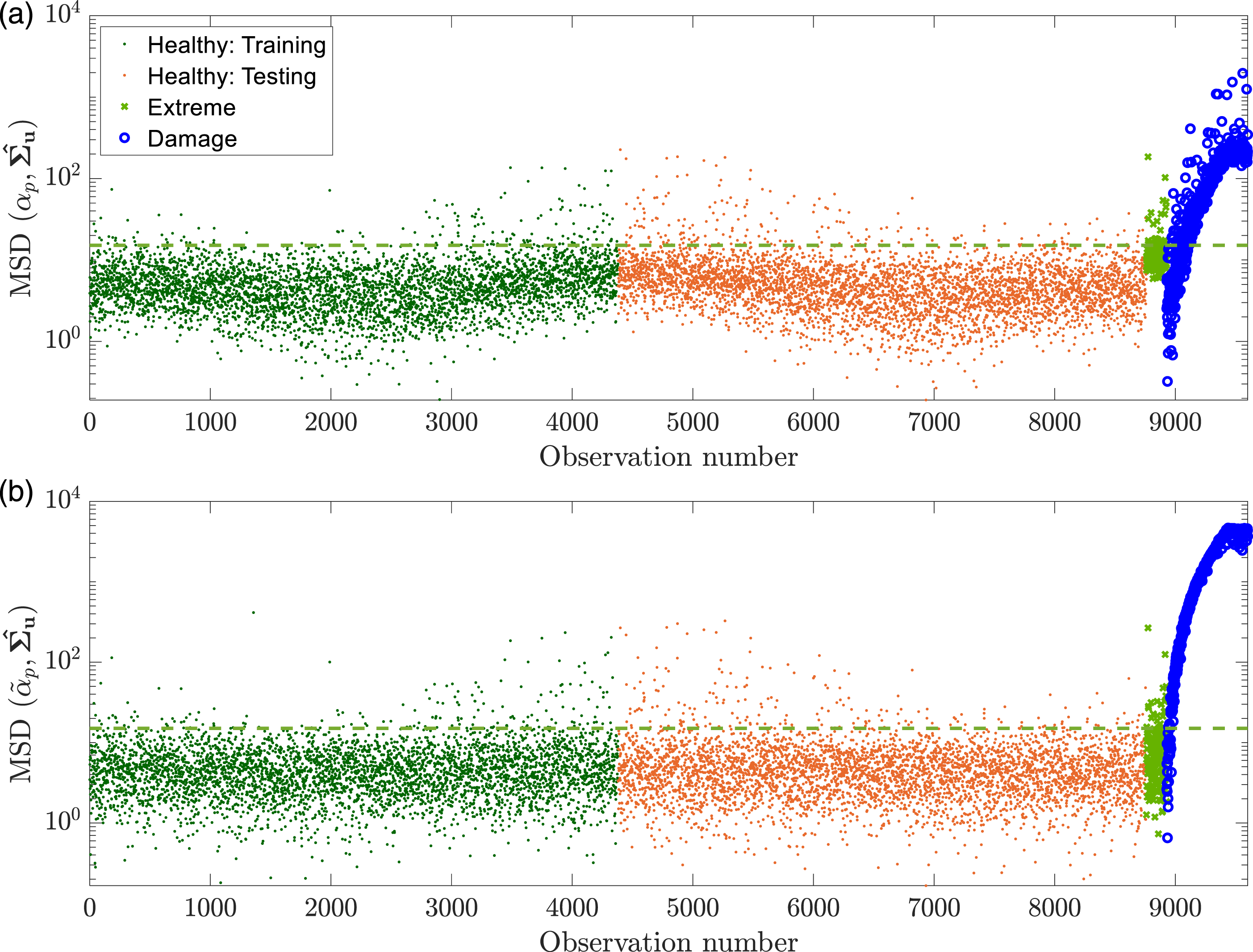
The objective of the regression models is to remove the influence that the EOPs have on the system. By studying the MSD for training and validation before correction, an obvious trend is present which correlates well to the temperature curve shown in Figure 1(b). Looking at the same region in the corrected features reveals that the trend is no longer present. Unlike the measured features, the behaviour of the extreme weather for the corrected features is now far more similar to that of the other undamaged observations. Rather being to the top end of the spectrum along with other observations of high temperatures, the observations now fall in line with both the testing and training observations. Perhaps the most significant change comes in the damaged observations. There is a clear difference between the measured and corrected features, most notably, the reduction in variability as the damage progresses. Given the reduction in variation across all the conditions, it can be said that the regression models perform their task of removing the influence of the EOPs. Although the damage detection has not significantly improved, the corrected features provide a more robust system with less sensitivity to the varying environmental and operational conditions. In order to get a more quantitative understanding of the improvement, Receiver Operating Characteristic (ROC) curves are plotted in Figure 4 for three scenarios. Firstly, for the testing compared to training, then for extreme weather compared to testing and, finally, for the damage compared to the testing. ROC curves to show improvement for corrected features over measured features. (a) Training compared to testing, (b) extreme weather compared to testing and (c) damage compared to testing.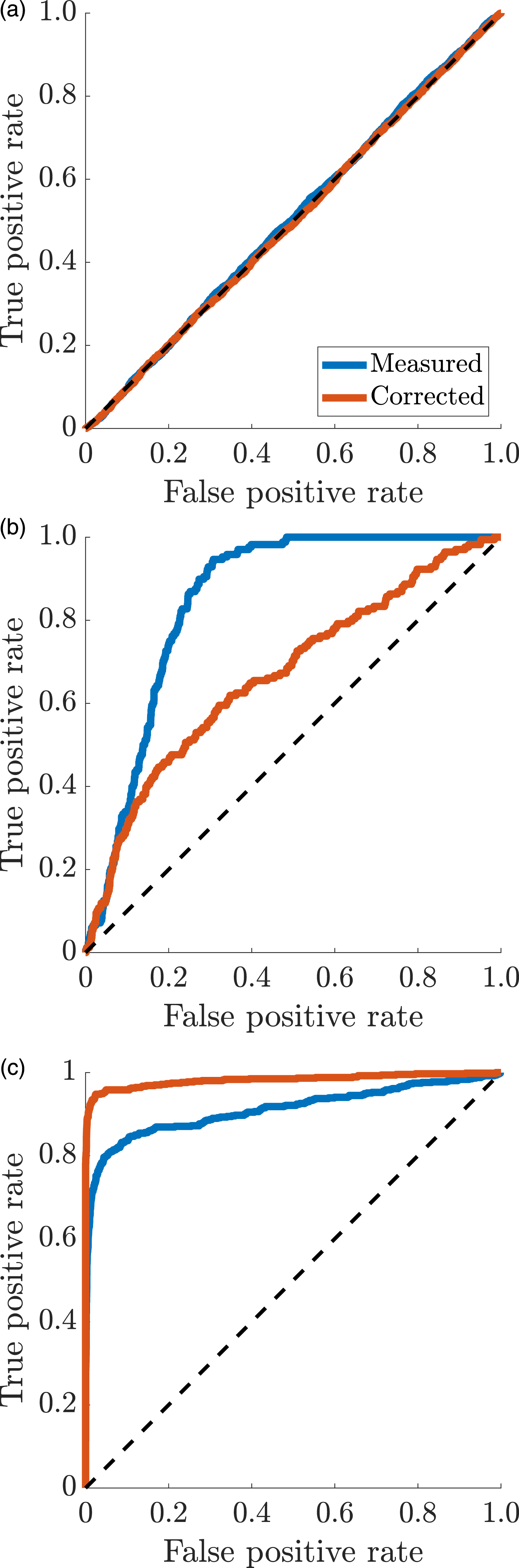
Considering first Figure 4(a), it can be seen that both the measured and corrected follow the diagonal between 0 and 1. This suggests that the overlap between the training and testing is near perfect and the two groups behave in the exact same way. Since the extreme weather observations are also undamaged, it would be desirable to witness the same effect in Figure 4(b) as Figure 4(c). However, due to the higher temperatures, the system does not see the observations as the same. In this case, the corrected features far outperform the measured features since the line is much closer to the 0 to 1 diagonal. This result shows that regression models have removed mostly the influence of the EOVs since the corrected extreme weather features perform more similarly to the training than the originals. Figure 4(c) shows a large improvement in the detection of damage. The corrected features are almost able to perfectly distinguish between undamaged and damaged observations. The reason it is not perfect is due to the very small damage at the start being very similar to the undamaged observations.
Another aspect to Figure 3 is that there are a significant number of outliers present, in both measured and corrected, across all the undamaged conditions (training, validation and extreme weather). However, a method can be introduced to explain these. Referring to Figure 2, there are a number of points that are positioned far above the general trend for each natural frequency. Figure 5 shows the corrected values for healthy training and damage for natural frequencies 4 and 6. Since Figure 5 is also plotted against temperature, it can also be seen how the regression has removed the trend with respect to the temperature. Regression corrected features for both healthy training and damage are plotted against temperature with outliers highlighted with red circles for corrected natural frequency (a) 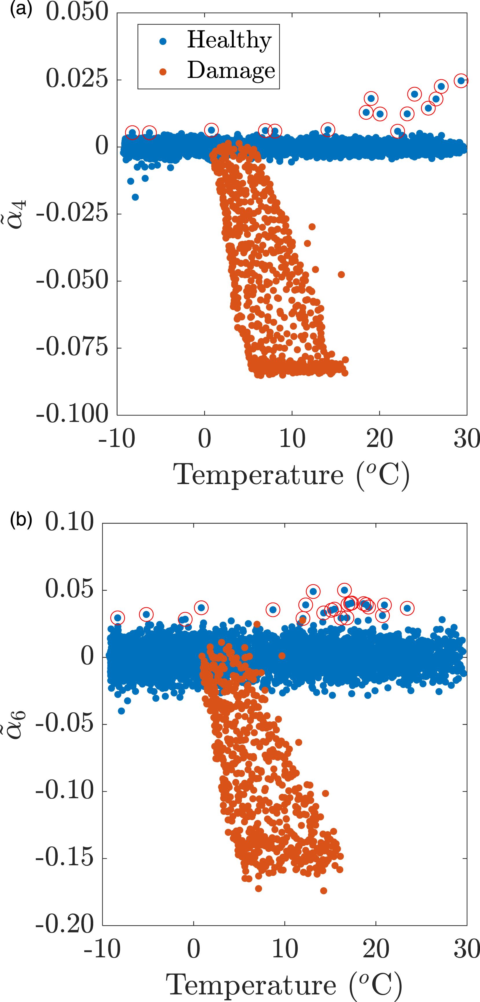
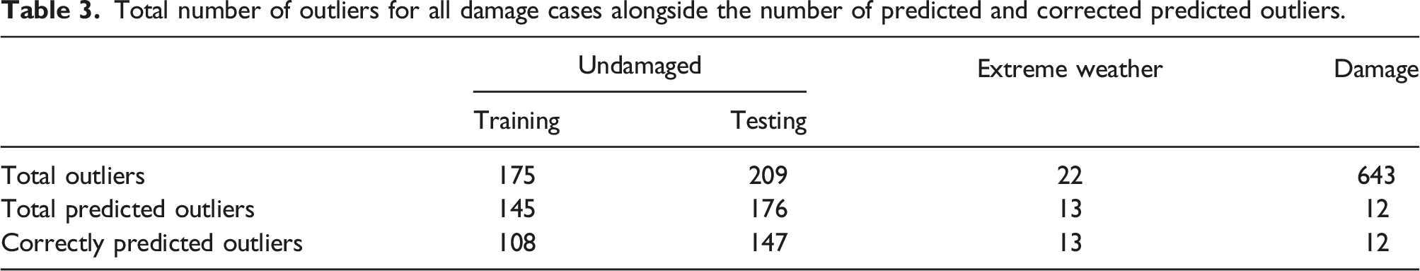
Figure 5 also shows that damage causes the stiffness to reduce, and hence the natural frequency. As such, it is possible to create a system to account for the benign outliers based on the corrected values that are well above their expected value. The outliers below the expected value are more difficult to predict, as they might be confused for damage. Highlighted with red circles are the observations where the value is more than 3 standard deviations above the mean of the healthy training. Tying this in, benign outliers can start to be identified based on poor estimations of the natural frequencies. Figure 6(a) shows which of the outliers in Figure 3 can be identified as outliers using the described system. Figure 6(b) instead shows how the control chart would look if the predicted outliers are discarded. Control charts showing and highlighting predicted outliers in (a) and removing them in (b).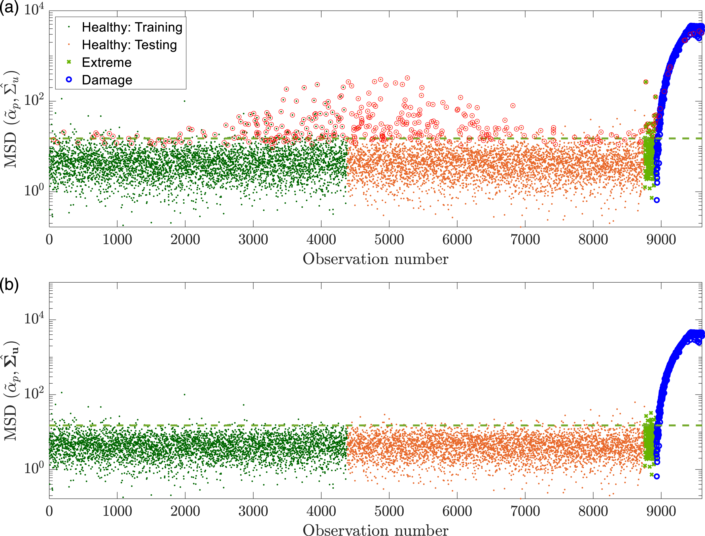
Total number of outliers for all damage cases alongside the number of predicted and corrected predicted outliers.
In summary, the regression models along with the natural frequencies features works well as a damage detection method. The regression corrected features outperform the measured features as they remove variations that are present because of varying environmental and operational conditions. An important thing to note is that when choosing the number of training points, enough observations were chosen such that the full range of temperatures and wind speeds, in the training data, were included so that the models could learn the relationships. A small issue arose with outliers but this was accounted for by studying the features in more detail.
Real Wind Turbine Blade
System Description
The data for the real turbine was taken from a piece of collaborative work carried out between the Technical University of Denmark and Brüel and Kjær on an operational Vestas V27 wind turbine. A more detailed description of the experiment can be found in previous works.
14
However, a short description is included in this work for the sake of completeness. During the experimental regime, a single blade was fitted with 12 accelerometers along with an electro-mechanical actuator at the root of the blade (see Figure 7). In this work, only eight accelerometers are used, namely, those found on the leading and trailing edges. The actuator was used to excite the blade and the accelerometers to record the vibrational response. Vestas V27 wind turbine VSHM set-up; (a) in-situ implementation, (b) a diagrammatic representation of the measuring equipment including accelerometers and actuator and (c) 45 cm crack on trailing edge of the blade.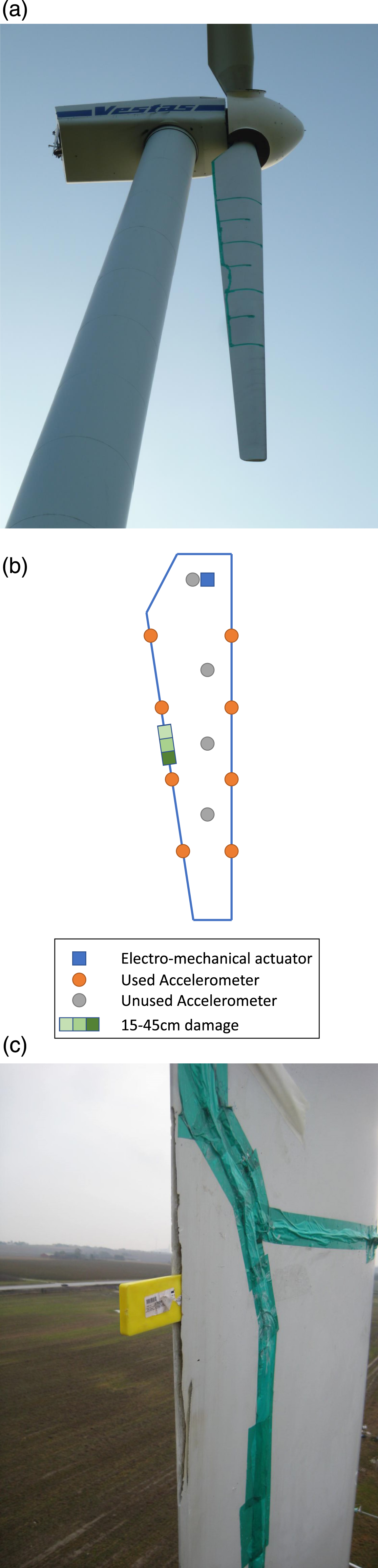
To be able to test the capabilities of a new VSHM procedure, the WTB was tested under five different states. These included an undamaged state, three damaged states and, finally, a state in which the introduced damage had been repaired. The damage was incrementally added in the form of a crack, starting at 15 cm and ending at 45 cm, on the trailing edge of the blade. The crack was created by physically breaking the WTB by debonding the upper and lower shells of the WTB, as shown in Figure 7(c). This is used to represent delamination in the structure, a type of damage which causes an overall reduction in the stiffness of the blade. Since the V27 is an older model of turbine, it consequently only has three operational modes (idling, 32rpm and 43rpm). For the analysis in this work, only the data obtained from the 43rpm mode will be used.
Since the turbine that is being analysed is located in a real environment, the instrumented blade was exposed to varying environmental and operational conditions. These conditions include (but are not limited to) temperature, wind speed, precipitation and azimuth angle. In an ideal situation, the reference state of the model would be trained on these parameters over the course of a full seasonal cycle to ensure a full range conditions was experienced and trained on. Consequently, a limitation is introduced into this work where the undamaged and damaged states may have experienced different ranges of conditions since the experiment lasted 4 months. As a result, the models created from the undamaged data might not transfer properly for the damaged data.
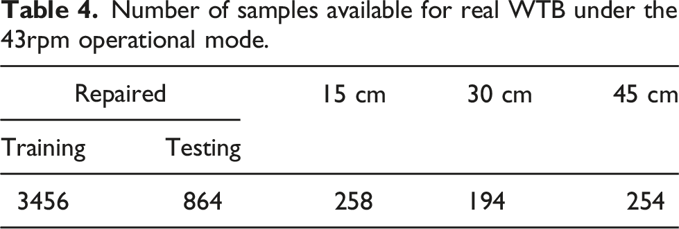
Number of samples available for real WTB under the 43rpm operational mode.
Frequency Transformation Based Features
From each observation, it is natural to create a single vector containing information obtained from an array of sensors. Unlike the natural frequencies, which combines information from all sensors, the frequency transformation based feature considers the input from each individual sensor in a single vector. A schematic of the derivation of the feature, for each observation, is given in Figure 8. However, a full mathematical explanation is also provided below. Schematic representation of the derivation of the frequency transformation based feature for each observation.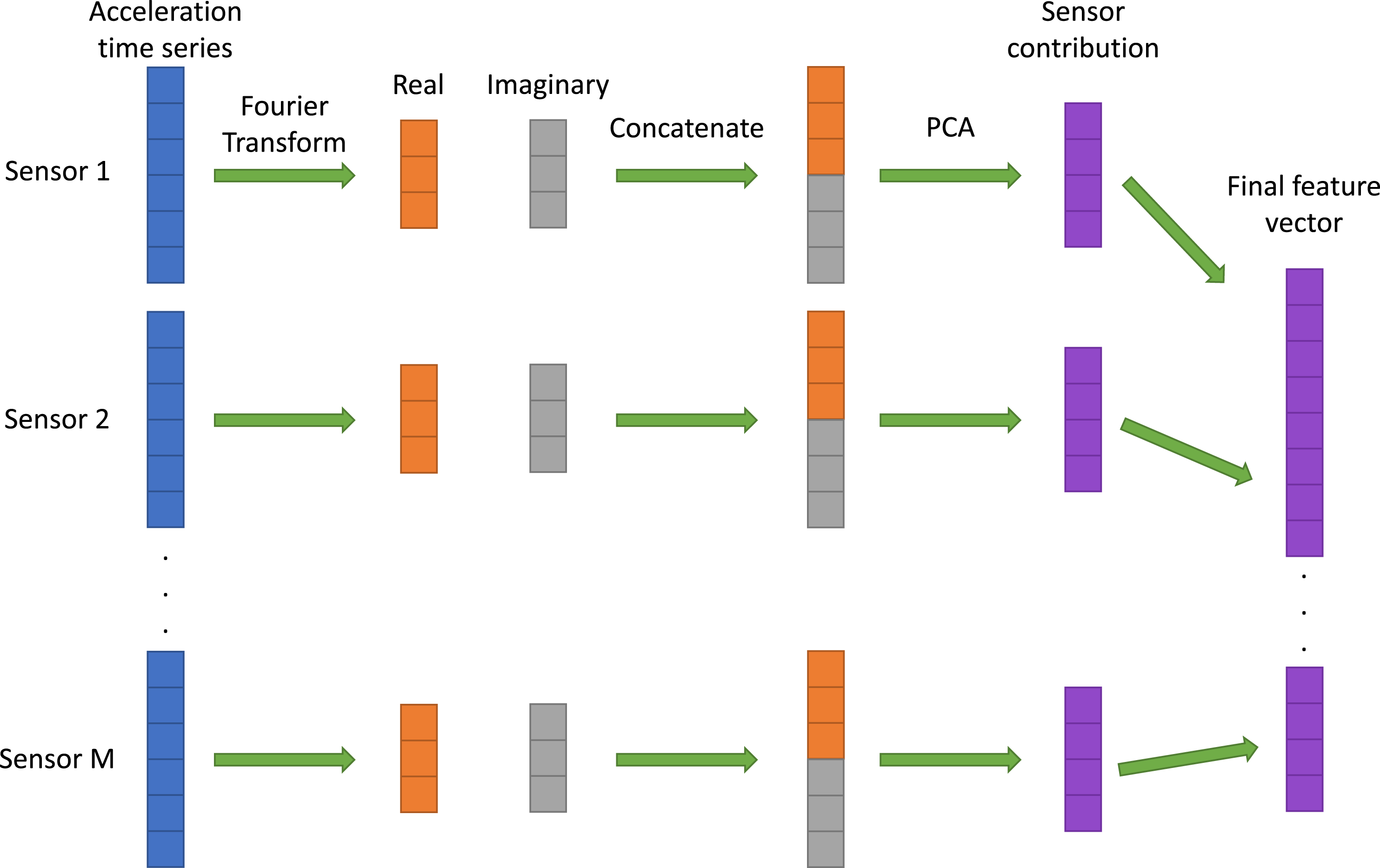
The data extracted from the sensors can be defined by the matrix
Once the data has been reorganised in this manner, a Fourier transform is performed on each time series vector individually. The Fourier transform brings the information from the time domain to the frequency domain such that 
Dimensionality Reduction

A reduced representation of the features contained in 
The final feature is then constructed by combining the information obtained from each sensor. In this work, the length of the reduced feature vector from each sensor is exactly equal since the number of PCs is considered, and kept constant, as opposed to the percentage variance they account for. An interesting variation on this method could be to create the final feature based on a total percentage of variation from each sensor. The final form of the feature for each observation, 
This holds true for all cases except where only a single Principal Component (PC) is used to project the information from each sensor. In this case, the individual reconstructions are a single value and, thus, the final feature for each observation is given by
System Analysis
As with the simulated system, it is important to first determine whether the DSFs have any discernible relationship between themselves and the EOPs. The EOPs that are tested in this analysis are temperature, wind speed, azimuth angle, the maximum acceleration and the standard deviation of the signal taken from the accelerometer adjacent to the actuator. The reason the frequency transformation based features are used in this case is because it was found, but not shown in this work, that the natural frequencies showed no identifiable relationships between the features and the EOPs. 20 The frequency transformation based features are conceptually harder than the natural frequencies, hence why they are not used for the simulated system. The frequency range extends up to 8194 Hz (Nyquist frequency), which goes far beyond the main structural resonances and comprises of a complex frequency spectrum. In addition, it has been shown that damage is better detected at higher frequencies. 20 Since the WTB is excited using an actuator, the frequency range is higher and, therefore, it makes sense to use a DSF that can exploit this fact.
Figure 9 gives examples of two different DSFs and how they can be corrected using multivariate nonlinear regression. For the first DSF, Figure 9(a), there is a clear relationship between itself and temperature. Since the first DSF is derived from the largest variance component, it is logical that it would be highly sensitive to temperature since temperature has a large influence on the overall stiffness of the structure and, hence, the dynamics it exhibits. However, once the feature has been corrected using the regression models, Figure 9(b), the relationship that existed before is no longer present. The same can be said for the third DSF when looking at the relationship against the standard deviation of the actuator hit before, Figure 9(c), and after, Figure 9(d), correction. Since the third DSF represents the third PC of the first sensor, it shows that each individual hit of the actuator has a significant influence on the features. In both cases, there is a wide distribution of points even after correction. This is a consequence of the fact that the models are not perfect since EOPs might be being considered which have no influence or, similarly, EOPs are not being considered in this work which have a greater influence than those which are considered. EOPs that are used for modelling but have no influence on the feature will add noise since a relationship that does not exist will try to be created. Trend of the first feature (first PC of first sensor) against temperature (a) before and (b) after correction using multivariate nonlinear regression. Trend of third feature (third PC of first sensor) against the standard deviation of the actuator impact (c) before and (d) after correction.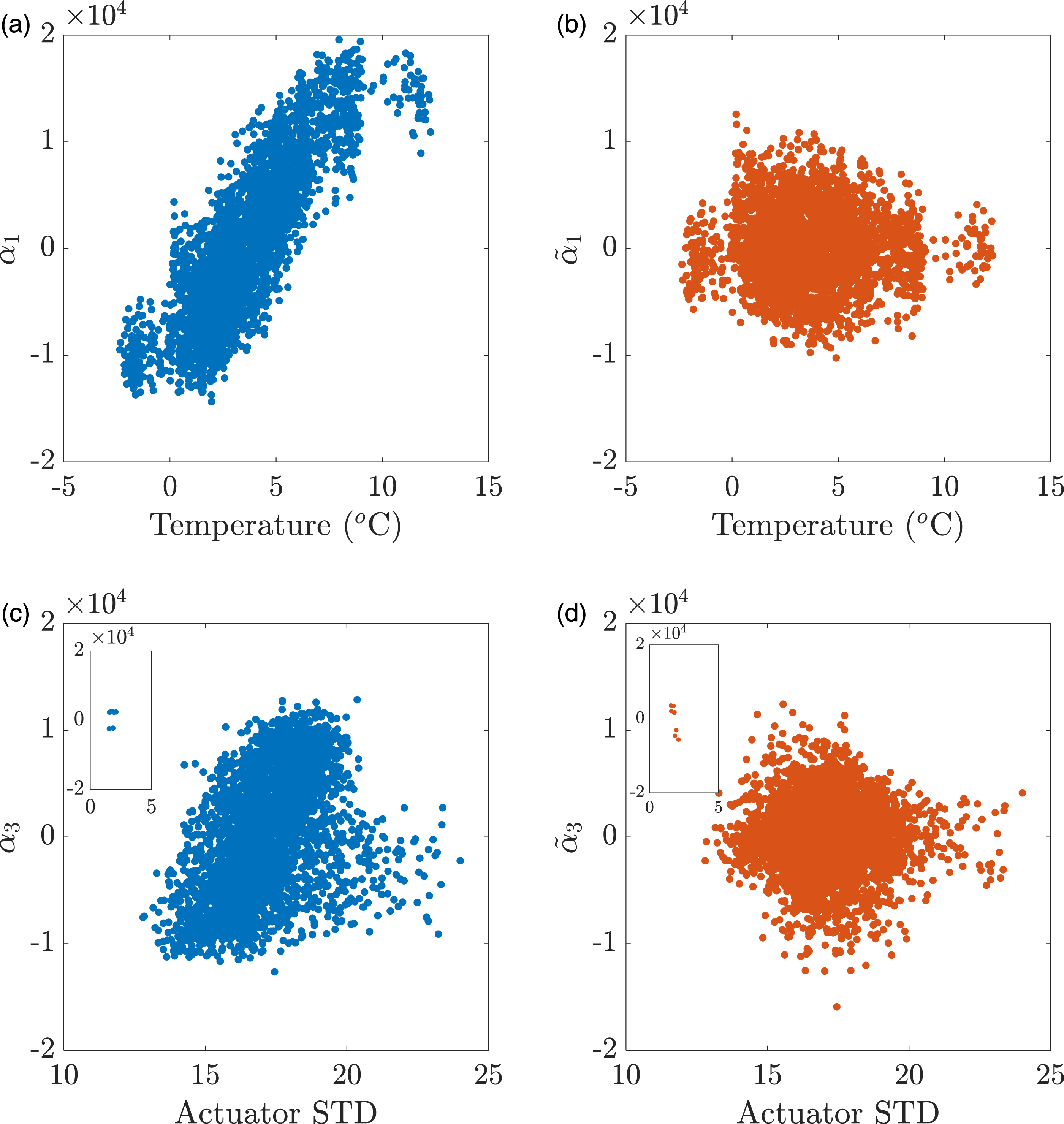
Once the features have been corrected using the regression models, their performance can be compared to the measured features to show if they have been improved. Firstly, it is desirable to see whether the correction in the features transfers through to the damage indices. The MSD in this example is calculated based on a vector containing the first PC from each accelerometer. Figure 10 shows the MSD against the temperature for the training data for both the measured and corrected features. The temperature is used since it was already shown in Figure 9 that it has a large influence on this feature; it is also assumed that the first feature corresponding to each accelerometer is similarly highly influenced by temperature. In the direct comparison in Figure 10(a), there is a clear difference between the two features sets. For the corrected data, there is a clear advantage where the DSFs no longer increase dramatically after 5 degrees centigrade. However, it can also be seen that there is a greater distribution of data points for the corrected features in the 0–5° range. This drawback could be fixed by refining the method for selecting optimal models by reducing the influence that non-influential EOPs have on each feature. Figure 10(b) and Figure 10(c) show the measured and corrected features with the general trend of the MSD, respectively. Plot directly comparing the MSD and temperature for a feature is constructed from the first principal vector for each accelerometer, leading and trailing edge only, such that Z=8. (a) Direct comparison of the two distributions, (b) and (c) show the measured and corrected individually each with its own trend line.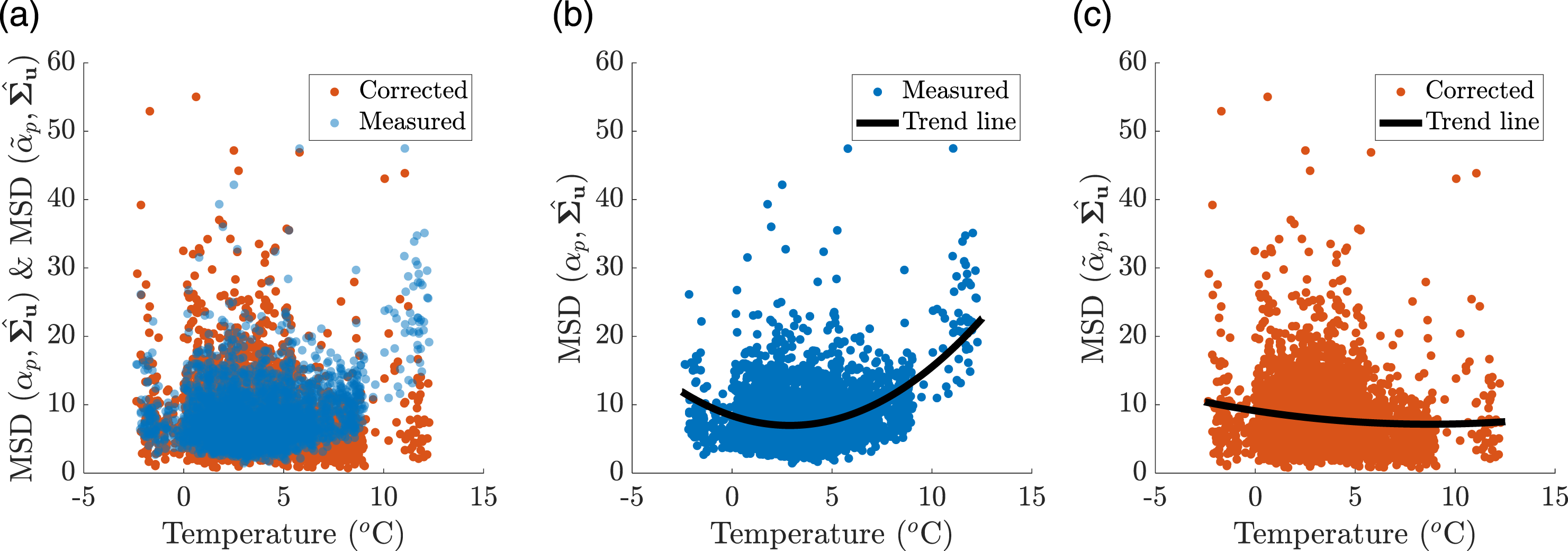
For the measured features in Figure 10(b), there is a distinct relationship between the temperature and the MSD. At both the lower and upper limits of the measured temperatures, there is a clear increase in the values of the MSD. This leads to a trend based on a strong temperature squared factor. Whereas, for the corrected features in Figure 10(c), there is much less increase in the MSD values at the upper and lower limits. This shows that the multivariate nonlinear regression corrects for the EOPs in, not only, the features but also in the MSD. This is important since the damage detection is based on the MSD and by removing the influence of EOPs, a more reliable system is created. This poses the question of why are the regression models used to correct the features rather than having one model to correct the MSD. It is the belief of the authors that if the influence of the EOPs remains embedded in the features, then the relationships between the EOPs and the MSD will become far more complex and difficult to model. In Figure 10, the trend is still clear but as more features are added to improve the damage detection, the relationship will become convoluted.
To compare the effectiveness of each method to detect damage, the control charts for each are plotted. To get a true understanding of whether there are benefits of using the regression models, two different scenarios are considered. The first scenario is for a method which looks only at the information obtained from a single accelerometer. Figure 11 shows the control charts for the measured and corrected features when considering only sensor 8. Control charts showing the capabilities of the method to distinguish between undamaged and damaged samples for (a) measured and (b) corrected features. Feature is constructed from only accelerometer number 8.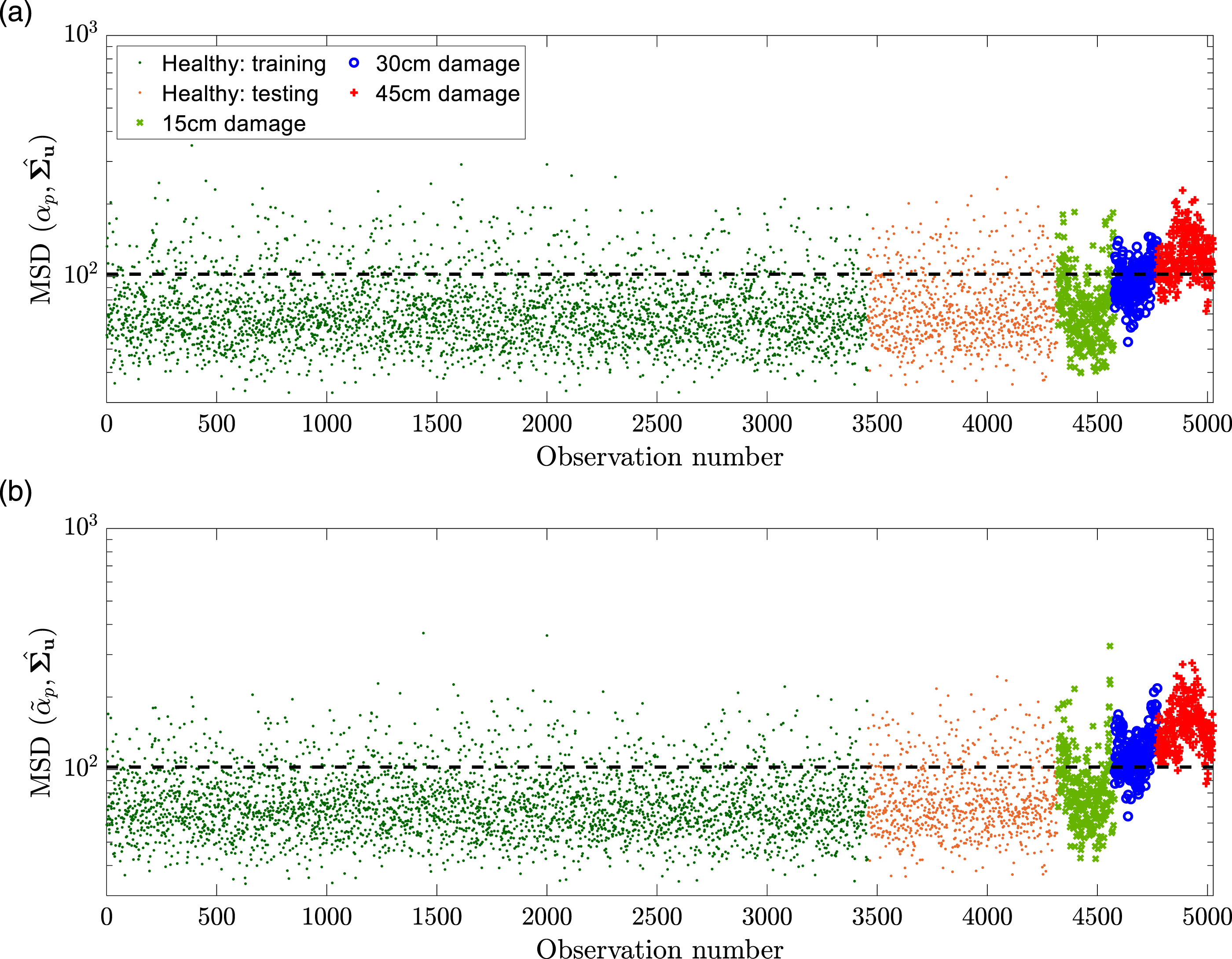
From Figure 11, it can be seen that there is a small but noticeable difference between the measured and corrected features. There are two main noticeable differences between them: firstly, there is a greater difference between the threshold and the damage and, secondly, there is much less overlap between the damage and the undamaged observations. The ROC curves in Figure 12 confirm these findings. From the ROC curves, there is a good improvement in the system’s ability to differentiate between undamaged and damaged observations when using the corrected features. However, a drawback that is evident in both cases is that there are a significant number of outliers within the undamaged observations. Additionally, neither the measured or corrected features are able to detect the initial damage of 15 cm. ROC curves showing false alarm rate for (a) 15 cm damage, (b) 30 cm damage and (c) 45 cm damage for information obtained from only accelerometer number 8.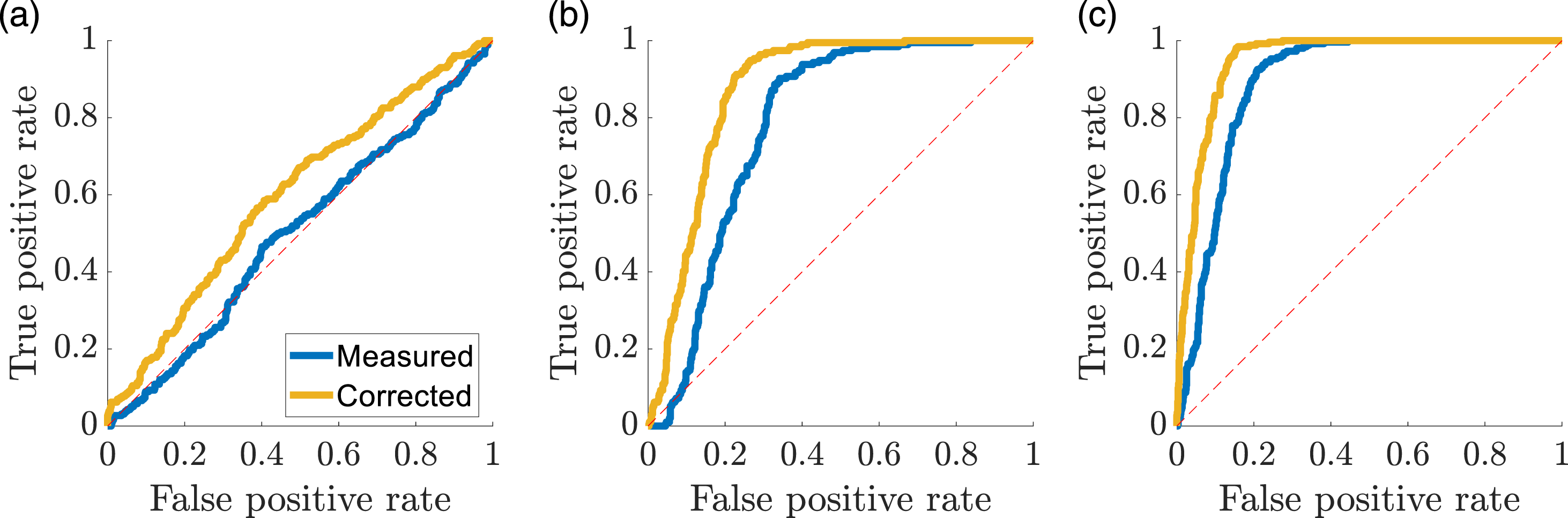
The control charts in Figure 13 show how the measured and corrected features compare when information from all eight accelerometers is considered. The most important difference between the feature sets is that damaged observations that are at the lower extremes have been captured by the main group, reducing confusion between undamaged and damaged. As before, there are a large number of outliers in the undamaged observations which, in the case of the corrected features, are more extreme. This effect could be a symptom of poorly fitted regression models which is an important issue that must be addressed in the application of the method on real structures. A benefit of using more information can be clearly seen in the difference between the threshold and the damaged observations. In Figure 13, the initial damage is detected where it was not before. In this case, it would be possible to increase it to 100% of the training data to reduce the number of outliers to nearly zero. However, this is dangerous because if a structure had experienced benign outliers during the training phase, it could lead to observations with higher MSD values and, thus, a higher threshold which could mask signs of early damage. As such, caution must be exercised to avoid such scenarios. Control charts showing the capabilities of the method to distinguish between undamaged and damaged samples for (a) measured and (b) corrected features. Feature is constructed using information obtained from 8 accelerometers.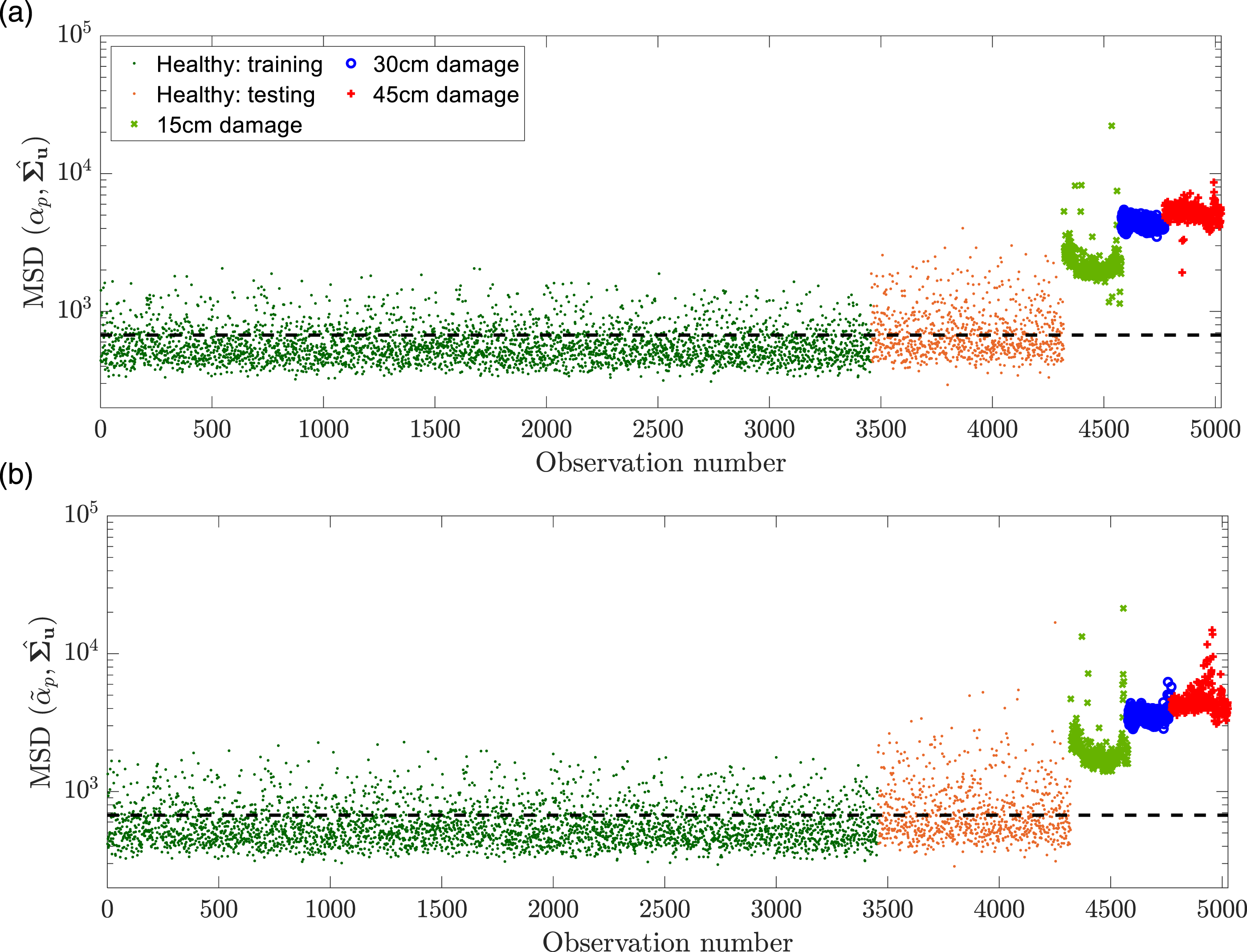
If the only goal is to increase the distance in the control charts, without considering outliers, between the undamaged and damaged observations, then the solution is to simply add more information through either more sensors or more PCs from each sensor. Adding more components increases the length of the feature vectors and hence the MSD since the distance in n-dimensional space will also increase, assuming the damage continues to affect the new features. However, caution must be exercised when adding more features since more and more noise will be added to the system and the baseline will become more distorted. Consequently, any further undamaged observations may appear different to those in the baseline.
The problem of choosing the number of components to include then can be considered to be an optimisation problem. It is a problem of optimising damage detection based on maximising the Area Under the ROC Curve (AUC) for the damage scenarios whilst simultaneously keeping the area between the baseline and the validation as close to 50% as possible. When the variation of AUC against number of PCs is compared in Figure 14, it can be seen that the regression corrected features can provide an advantage over the original features. Variation in AUC for (a) Validation/Training, (b) Validation/15 cm damage, (c) Validation/30 cm damage and (d) Validation/45 cm damage.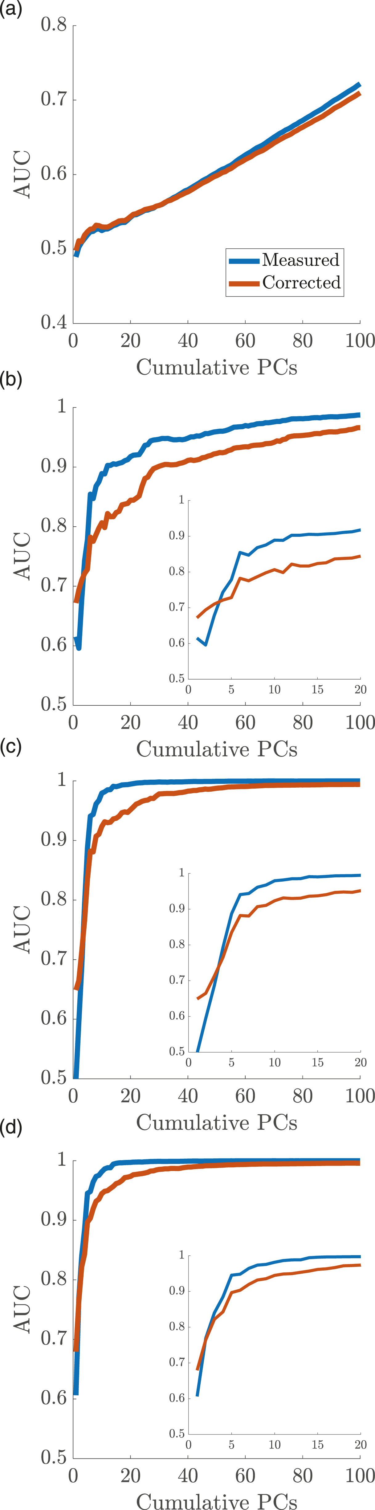
Figure 14(a) shows the AUC curve between the baseline and validation set changes with respect to the number of PCs used. For this case, it is desirable to have the baseline and validation behave in the same way and, as such, have an AUC as close to 0.5 as possible. It can be seen that the corrected features start closer to 0.5, and perform better as more information is added. A reason for this could be because of the feature that is being used. As the PCs explain less of the variance of the frequency transformation, they no longer correspond across all sensors meaning that they will be influenced differently by the EOPs. The corrected features then perform better because they are still able to remove the influence of the EOPs giving a more uniform distribution. Since the amplitude of the features will be similar, so will the corresponding features for the same numbered PC.
Across the three damaged scenarios in Figure 14, it can be seen that whilst the corrected features provide superior damage detection with fewer PCs, the measured features perform better overall. The most probable reason for this is that the lower PCs correspond to the features which are most influenced by EOVs. The corrected features perform better at lower PC numbers since they can differentiate between the undamaged and damaged observations by removing the influence of the varying conditions. However, it does not make sense to use so few PCs when better damage detection can be achieved by using more.
One potential reason for the decrease in AUC as PCs increase is that features are being regressed that do not require doing so. The higher PCs often correspond to noise and are not influenced by EOVs. By trying to regress these features, more uncertainty is introduced to the system. This could be addressed by using a measure to determine the corresponding benefit of the regression against no regression. The regressed and non-regressed features could then be combined to provide a superior method. A different reason for the decrease in the AUC could be related to development of the feature vectors in n-dimensional space. This problem is difficult to identify and address.
The purpose of using the regression models to correct the features is to bring more control into the overall system. They provide additional robustness by being able to handle observations that experience conditions in which the baseline was not trained with, assuming the defined relationships hold true over greater ranges. Since the regression models can show an improvement over a standard methodology, it is logical to apply them in any scenario where the features themselves can be shown that they are sensitive to changes in environmental and operational conditions.
Discussion
A simulated WTB was used to test the methodology in a controlled environment in order to evaluate the potential of using regression models to correct the DSFs. It was shown that the corrected features removed most of the variability in the damage index as well as correcting the extreme weather observations such that they behave the same as the other undamaged observations. Data from an operational wind turbine was then used to demonstrate the ability of the method on real data. Firstly, the DSFs were demonstrated to be sensitive to the varying conditions. The regression corrected features were shown to provide superior damage detection when less information from each sensor is considered. However, the potential regression of insensitive features proved to hurt the regression corrected system at higher number of PCs.
There are many points that have been raised in this work that must be considered when analysing the practicability of applying a VSHM method of this for long-term monitoring. Some of the issues have been addressed directly in this work and some must be looked into further. When such points have been reflected and worked upon, a more robust VSHM system can be created that may see implementation in the future of civil structures.
Outlier analysis
The first aspect that has been analysed is the problem associated with the large number of outliers present in the training data, due to the poorly estimated natural frequencies. In order for a system to be robust, it is important to be able to identify whether the outliers are benign or appear because of damage. If possible, the number of false positives and false negatives can be greatly reduced. In this work, the problem was solved by identifying the connection between the features and the outliers in the MSD. A method was implemented that aimed to identify outliers, which had a high success rate. By discarding the points that were found to be benign outliers, a more reliable system was created. Since this was tested on simulated data, the relationship was easier to identify and, therefore, implement. In more complex systems, such as the real WTB, the relationship between the outliers and the features will become more complex, future work should consider a methodology to identify and remove the influence of outliers in the data.
The DSFs from the real WTB also displayed a significant problem with outliers. The problem was worse in the case of the regression corrected features. The reason for this might be down to a limitation in the MSD but more likely due to DSFs that are being regressed which do not need to be. Regressing features that are insensitive to EOVs only leads to further uncertainty in the system. Any uncertainty is undesirable and can add more confusion for the system if it is left untreated. As such, effort should be put toward defining the most robust features possible.
Reducing data dimension
In this work, the problem associated with choosing the optimal amount of information from the vibration response to include for improved damage detection was studied. For the simulated blade, the decision was made to include the first six natural frequencies since they were well-defined and non-overlapping. With the addition or removal of natural frequencies into the system, more uncertainty or less information on the damage, respectively, may have been included. With regards to the real WTB, the decision on choosing the right number of PCs to include from each sensor is more complicated. From Figure 14, it can be seen that by increasing the number of PCs, it is possible to increase the damage detection rate but at the cost of increased separation between the validation and training sets. Since it is so important for the validation and training to appear the same, it becomes difficult to choose the number of PCs to select.
Remaining trends
Another aspect that must also be addressed is that there is still a trend remaining in Figure 10(c). Since the purpose of the regression models is to remove the influence of the EOVs, in an ideal scenario there would be no remaining trend between the EOPs and the DSFs or MSD. There exist several possibilities for why the trend still remains. Two such reasons revolve around the selection of EOPs for modelling. Firstly, EOPs might have been selected that bear no influence on the DSFs and when introduced in the regression introduces a bias. Conversely, it is also possible that there are unmeasured EOPs that are still influential but cannot be introduced into the model. Other reasons may relate to the way in which the model orders are selected. Resolving these problems will most likely have the effect of reducing the distribution of the MSD points for any particular damage scenario. These issues will be addressed in future work.
Conclusion
Multivariate nonlinear regression was implemented to correct DSFs obtained from simulated and operational WTBs. The corrected DSFs can provide superior damage detection compared to a standard PCA-based system as well as providing increased stability. However, the main contribution of this work was to address some of the practicalities of applying multivariate nonlinear regression to real, operational structures. A number of practical aspects were considered, including determining whether outliers were benign or damage, reducing the amount of data to the essential information for damage detection and reducing the number of EOPs used as inputs to remove any remaining trends as well as reducing variability in DSFs.
There are many aspects that still need to be addressed in order for this type of method to see implementation. A method needs to be developed to improve the regression models to give more reliable outputs to reduce the variation of points and to completely remove any trends. In order to further reduce the amount of data, and to emphasise the important information, the DSFs could be further analysed and broken down further. Additionally, the quality of the training data could be improved by increasing the number of observations that are used and by removing the influence of benign outliers.
Footnotes
Acknowledgements
The authors would like to acknowledge The Carnegie Trust for the Universities of Scotland for their support in the work through the Caledonian PhD Scholarship (grant reference number: PHD007700). In addition, the authors would like to thank Dr. Dmitri Tcherniak for providing advice and data from the V27 wind turbine monitoring campaign. For the purpose of open access, the author has applied a Creative Commons Attribution (CC BY) licence to any Author Accepted Manuscript version arising from this submission.
Declaration of conflicting interests
The author(s) declared no potential conflicts of interest with respect to the research, authorship, and/or publication of this article.
Funding
The author(s) disclosed receipt of the following financial support for the research, authorship, and/or publication of this article: The Carnegie Trust for the Universities of Scotland for their support in the work through the Caledonian PhD Scholarship (grant reference number: PHD007700).