
Abstract
With the growing number of well-aged bridges and the urgency in developing reliable, (pseudo-) real-time monitoring of structural safety and integrity, there is a worldwide and widespread campaign toward transforming structural health monitoring practice. Among these attempts, the application of data-driven approaches in developing damage identification techniques has received particular attention in recent years. Given the growing volume of structural health monitoring data, the power of data-driven approaches has been further exploited. These efforts have been predominantly focused on building and training algorithms using direct measurements from bridges. Although recent years have seen transformative technologies in producing cheap and wireless sensors, network-wide bridge instrumentation is logistically difficult and expensive. This has led to a new group of structural health monitoring systems entitled indirect or drive-by approaches. In drive-by systems, measurements from an instrumented vehicle are used to extract structural damage signatures. In other words, in these systems, the instrumented vehicle acts as both actuator and receiver while passing over a bridge. The main challenge in deploying drive-by approaches for damage identification purposes is that the signals collected on drive-by vehicles also embody signatures from the vehicle, road/rail profile and are easily contaminated by environmental and operational conditions. Furthermore, the majority of current drive-by damage identification systems rely on prior knowledge of vehicle or bridge dynamic characteristics which has led to limited application of the concept in practice so far. To address these challenges, this study employs a powerful class of deep learning algorithm to develop a damage identification system using measurements on an instrumented travelling train. The proposed algorithm is capable of automatically extracting damage signatures from train-borne measurements only. To demonstrate the algorithm’s capability, the method is applied to measurements collected on a model instrumented train travelling on a simply supported model steel bridge. For this purpose, a deep convolutional neural network is built, optimised, trained and tested to detect damage using acceleration signals collected on the instrumented train only. The hyperparameters of the algorithm are optimised using the Bayesian optimisation technique. The accuracy of the algorithm is experimentally tested for four positive damage scenarios (combination of two different locations and intensity) and three different travelling speeds. This is the first demonstration of the data-driven drive-by damage identification system under scaled operational environment conditions. The performance of the proposed method is discussed under different travelling speeds and different damage states. The result shows that the proposed method can accurately and automatically detect and classify damage under varying speed, rail irregularities and operational noise using train-borne measurements only and offers a great promise in transforming the future of bridge damage identification system.
Introduction
Traditional bridge inspection methods are often subjective to inspectors’ level of expertise and can be prone to data degradation as there rarely exists a systematic framework for data collection. The ever-growing urgency in devising a reliable, automated, (pseudo) real-time structural health monitoring system has led to an increasing volume of studies utilising direct instrumentation of bridges for damage detection, localisation and prediction of remaining service lifetime. While direct instrumentation addresses the subjectiveness of visual inspections, the instrumentation and maintenance of the acquisition system challenge the sustainability of direct monitoring on a long-term and network-wide scale. Furthermore, direct structural health monitoring often requires a calibrated structural numerical model and relies on prior knowledge of damage-prone areas, leading to a bespoke system specific to a particular bridge at a certain location. These challenges collectively led to a paradigm shift in structural health monitoring, which is entitled indirect structural health monitoring (SHM) systems.
Indirect SHM systems cover a wide range of approaches, from drone-based visual inspection to extracting bridge vibration signals using measurements collected on an instrumented passing vehicle (drive-by concept). In a drive-by approach, an instrumented vehicle acts as both actuator and receiver while passing over a bridge. The indirect drive-by SHM systems offer an advantage to vision-based damage identification systems as the vehicle-borne signals can manifest changes due to structural damage on a bridge and provide insights into the effect of the damage on the global behaviour of the structure.
Yang and co-authors 1 introduced the application of the concept of drive-by damage identification system by demonstrating the feasibility of extracting bridge frequencies from acceleration signals on a passing vehicle. The experimental validation of the concept was investigated using a one-axle cart. 2 Yang and Yang 3 have extensively reviewed the developments in the drive-by concept in the last decade. Their review shows that the majority of the drive-by damage identification systems have focused on identifying shifts in natural frequencies of the structure under consideration. According to Malekjafarian et al., 4 the optimal conditions for extracting bridge frequencies are low drive-by speed (less than 25 mile/h), smooth road profile, multiple crossings and use of a heavy instrumented vehicle. The speed of the vehicle not only influences the length of the signal while passing over the bridge but also changes the excitation level. Similarly, the road/rail profile can excite the vehicle further and mask the damage-induced signatures in the signal. Multiple crossings and the use of heavy vehicles could help to address these issues to some extent; however, these shortcomings can limit the network-wide application of the concept.
While natural frequencies of a bridge can offer useful insights into the existence of damage, their sensitivity to environmental and operational conditions (e.g. varying temperature and vehicle mass) has led to studies that have utilised other modal parameters as damage sensitive features. Among these attempts is the study conducted by Yang et al. 5 in which Hilbert amplitude of the filtered vehicle-borne acceleration is used to extract bridge mode shapes. In addition to their sensitivity to environmental and operational conditions, one of the main challenges with an indirect mode shape-based damage detection system is reported to be the required signal length, which challenges the applicability of the system for short- and medium-span bridges, under operational speed. 6 Another challenge is the necessity for prior knowledge and understanding of mode shapes in normal/healthy conditions to help identify anomalies induced by damage.
There are also several attempts in developing indirect damage identification systems without the explicit use of bridge modal characteristics. For example, OBrien et al. 7 have used moving force identification to monitor the damage state of the bridge using vehicle-borne acceleration and calculating road surface profile and global bridge stiffness. Their method relies on prior knowledge of the dynamic characteristics of the vehicle. In the study conducted by Quirke et al., 8 an optimisation technique is deployed to calculate the apparent profile as a damage sensitive feature using vehicle-borne acceleration measurements. Furthermore, a growing number of research studies have focused on using wide-ranging signal processing tools such as Morlet Wavelet, Mexican Hat Wavelet, Continuous wavelet and Hilbert transform to extract damage sensitive features from vehicle-borne acceleration signals.9–12
While there is a significant body of research on applying the drive-by concept in developing a damage identification system, the majority of the studies have focused on theoretical and experimental model-based (numerical model of the bridge) SHM systems with no/limited consideration of varying operational and environmental conditions. A model-based system detects damages using a mathematical bridge model and physical description of the structure behaviour. The difference between the measured response from the vehicle and the expected response from a healthy model is then used to assess the damaged state of the structure. On the other hand, a model-free system relies on analysing the bridge behaviour without developing a numerical model of the structure, using a data-driven algorithm. The latter approaches generally provide limited insights into the physical interpretation of damage; however, they offer great potential for network-based real-time SHM. The recent breakthroughs in exploiting the computational capabilities of machine learning-based approaches have paved the way for wide-ranging applications of these methods in the structural health monitoring field. The availability of high-performance computational capacities and the growing bulk of datasets have also been great contributors to the wide-ranging application of model-free techniques in developing semi-automated SHM systems.
In the context of drive-by studies, there are very few attempts in utilising the power of machine-learning-based algorithms. To the best of the author’s knowledge, the study conducted by Malekjafarian et al. 13 and Locke et al. 14 are the only two studies in which a form of machine-learning-based algorithm is used to develop a model-free drive-by damage detection system. Malekjafarian et al. 13 have built a relatively shallow neural network using simulated vehicle-borne acceleration from multiple passing and Discrete Fourier Transform spectrum of the acceleration as damage sensitive features. In the study conducted by Locke et al. 14 frequency spectrum of simulated acceleration signals is used to build and train a one-dimensional (1D) deep learning algorithm. The current study presents the very first two-dimensional (2D) deep learning-based drive-by damage detection system, tested under scaled operational conditions.
Among wide-ranging machine learning algorithms, deep learning architectures have shown great promise in automating structural health monitoring processes. A typical deep learning algorithm consists of feature extraction and classification component. As the name suggests, the former component utilises a wide range of signal processing techniques to extract features/indicators most sensitive to damage. In the second component, extracted features are mapped against corresponding damage classes. In a damage detection algorithm, the classes are limited to healthy and damaged states, while for the localisation algorithm, the classes will expand to cover classification for different severity and location. Since the performance of a deep learning algorithm is a function of both its components, integrating the feature extraction and classification into one unit body of learning can improve the efficiency of the algorithm. This notion is the underlining fundamental of a powerful class of deep learning algorithms entitled convolutional neural networks (CNNs).
Similar to the visual cortex’s functionality in the object detection process, the learning in CNN algorithms is based on collating information from neighbouring inputs to build sub-features, helping to accentuate distinguishing and discriminating differences in multiple classes. Given the integration of feature extraction and classification components in one unit architecture, CNN algorithms are computationally much more efficient than traditional shallow neural networks.
To this point, the application of CNN algorithms in developing damage identification systems has been limited to vision-based monitoring such as the studies conducted by the authors of Refs. 15–18 in which high-resolution images are used for crack detection purposes. In the context of vibration-based damage identification systems, the attempts have been focused on resizing a 1D into 2D images 19 or building a 2D image using measurements from multi-instrumentation. 20
In this study, the transfer learning technique is used to adapt GoogLeNet, one of the most powerful pre-trained CNN algorithms, for drive-by damage identification purposes. GoogLeNet utilises parallel filters to enhance multi-scale representation without compromising on computational costs. This is facilitated using inception modules which expand the receptive field by stacking filers in parallel paths. 21 Multi-scale feature extractors use a large range of receptive fields to describe context at different scales 22 and in CNN architecture, the learning body learns coarse-to-fine multi-scale features through a stack of convolutional operators. 22 The receptive field in deep learning terminology refers to the input space that influences a particular unit of the network.
GoogLeNet’s unique network-in-network architecture stacks multi-layer perceptron as micro-networks into a large network to improve the discrimination power of the algorithm in local zones of a receptive field. The number of layers and learning units in a convolutional neural network architecture significantly influences the performance of the algorithm; however, deep networks may suffer from the risk of overfitting, exploding/vanishing gradient problem and computational cost. The network-in-network architecture leads to a significant increase in depth of the architecture without significant compromise on computational cost. The inception modules in GoogLeNet use convolutional layers with different filters for multi-scale feature detection and reduce the computational cost through dimensionality reduction. To this point, GoogleNet’s application has been limited to computer vision tasks such as object detection, face detection and recognition. To the best of the author’s knowledge, GoogLeNet has never been used for SHM purposes.
In this study, GoogLeNet’s architecture is used as the backbone of the learning body. Transfer learning is then applied to train and re-purpose the algorithm for drive-by damage detection and classification purposes. The algorithm is trained and tested using instrumented model train passing over a model steel bridge. This is the first scaled practice-based proof-of-concept for a data-driven drive-by damage identification system. In this study, the spectrogram of measured train-borne acceleration signals, without any additional pre-processing, is used as the initial damage sensitive feature.
The proposed method in this study exploits the fusion of multi-level and multi-scale capability of GoogLeNet learning architecture and re-purposes this well-known CNN algorithm for SHM applications. The proposed methodology offers an end-to-end damage identification system by eliminating the need for an additional and subject matter expert signal pre-processing. The proposed learning body does not make any assumption on the speed of the vehicle or the geometry of the structure.
The following sections provide an overview of the methodology and the architecture of the adapted GoogLeNet algorithm and the utilised Bayesian optimisation process to fine-tune the hyperparameters of the learning body. Then details of the testing environment, the model train and bridge and specification of the instrumentation equipment are presented. This is followed by the process of building, training and testing of the algorithm and conclusion remarks.
Principle of convolutional neural network and GoogLeNet deep learning architecture
As mentioned in the introduction section a typical CNN architecture consists of two main components of feature selection and classification. Figure 1 schematically demonstrates the basic structure of a typical CNN learning body. The feature classification component of a CNN algorithm contains layers of convolution, pooling and activation filters. In deep learning terminology, patch/filter size refers to the size of the sweeping/kernel window in both convolution and pooling layers and the number of strides defines the amount of shift in the sliding window. The functionality of convolution layers is similar to that of digital filters by converting an image into a new filtered image, also known as feature maps. The purpose of these filters is to accentuate the distinguishing and discriminating features of the input image. On the other hand, the pooling layers reduce the dimension of the input image by combining the neighbouring pixels into a single pixel, hence optimising the computational costs.
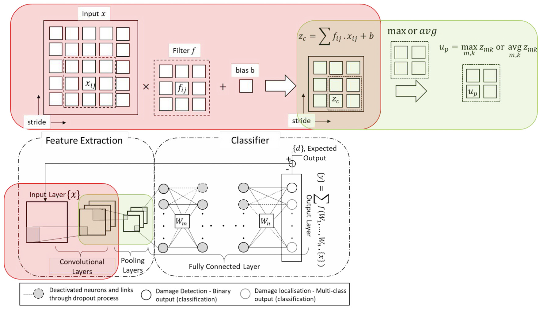
Schematic demonstration of a typical convolutional neural network architecture.
The architecture of the second component of a CNN algorithm is similar to a typical multi-class neural network with hidden connected layers and an activation layer. In order to avoid the risk of overfitting, dropout layers (i.e. randomly zeroing activations and nodes/weight deactivation during the forward pass in training) are often added to the architecture of the classification network.
Generally, the depth of a CNN structure defines the performance of the algorithm, as deeper architecture offers better accuracy but with a significant increase in computational costs. Hence, the trade-off between accuracy and computational cost has led to numerous attempts in developing a balanced architecture. Among such attempts is the GoogLeNet model developed by Szegedy et al. 21 The 22-layer deep GoogLeNet’s architecture consists of 60 convolution layers with a network-in-network structure. In network-in-network architecture, additional 1×1 convolutional layers are added to increase the depth and width of the network without compromising on computational costs or the accuracy of the algorithm. 23 In GoogLeNet, different convolution and pooling filters are combined in a wide architecture to extract more information into smaller layers. This structure is referred to as inception modules. Figure 2 shows an example of an inception module. Another main feature in GoogLeNet is its use of sparsity as opposed to a fully connected layer which supports reduction in computational costs and risks of overfitting associated with fully connected layers.
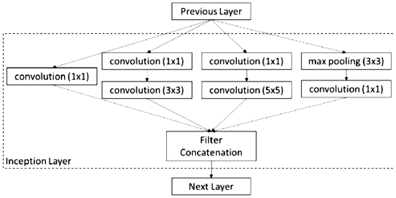
Inception layer with dimensionality reduction (adapted from Ref. 21).
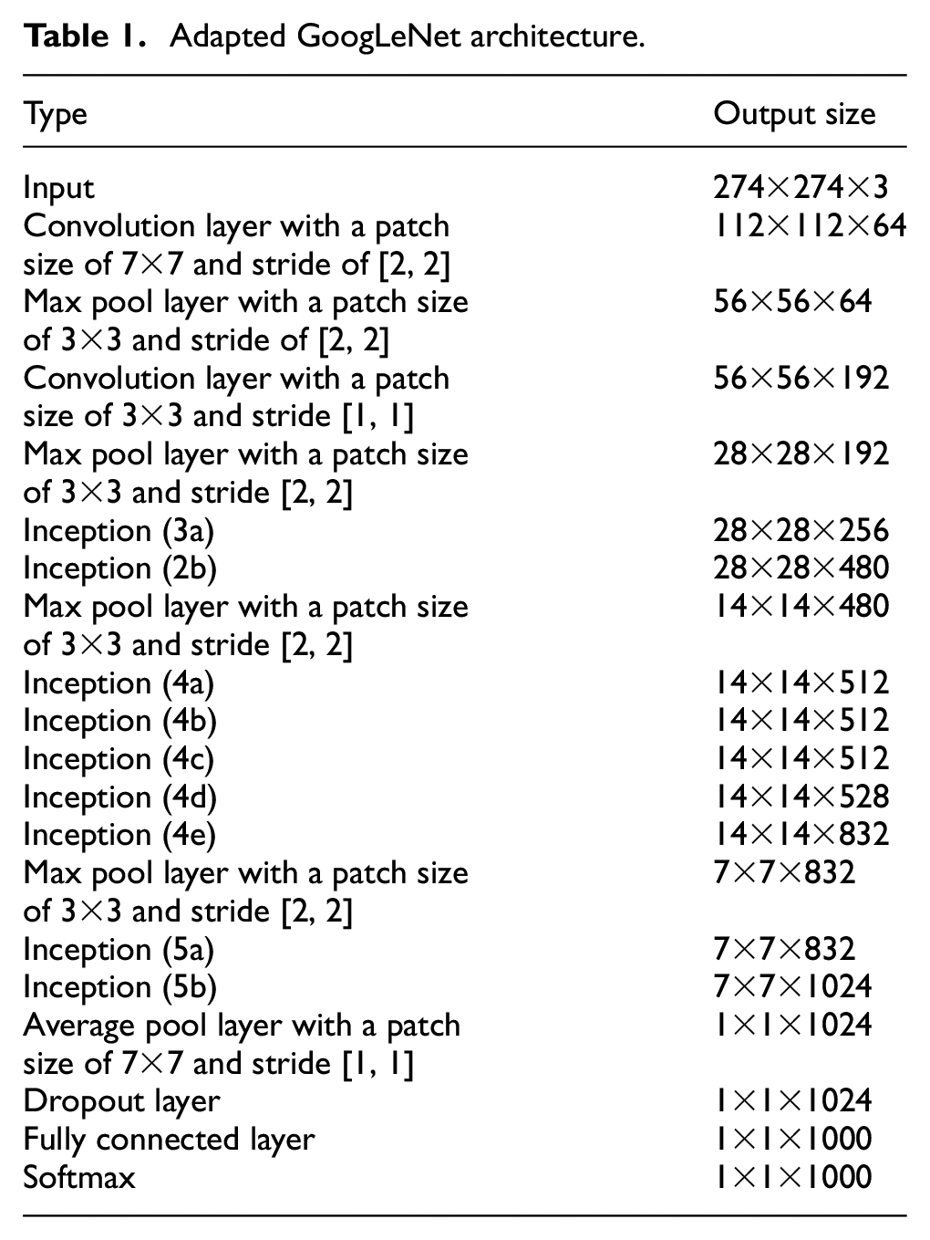
Given GoogLeNet’s power in image classification, the transfer learning technique 24 is employed to train the algorithm for drive-by damage identification purposes. Transfer learning allows the exploitation of the pre-trained knowledge and re-purposes the algorithm for other applications without training a very deep CNN algorithm from scratch. Table 1 summarises the structure of the CNN structure adapted in this study. In each layer, the output size represents the output dimensions of each layer after the input is passed through that layer. Each inception layer is a stack of 1×1, 3×3 and 5×5 convolution filters. As can be seen from the output size in each layer, the graphical dimensions reduce as the feature dimension (third dimension) increases. As mentioned before, the pooling layers (max or average) also reduce the spatial dimension by downsampling, using the maximum or average values of the receptive field.
Adapted GoogLeNet architecture.
The fully connected layer function is similar to that of a convolutional layer with a filter size of the input; hence, the output spatial dimensions are reduced to 1×1. In order to reduce the risk of overfitting, a dropout layer is added to disconnect the connections and deactivate neurons. The last and final layer in the network is a softmax layer. The functionality of the softmax layer is to normalise the input vector to return the probability for each individual damage class. For supervised damage detection, two classes of healthy and damaged are of concern, and for damage classification, multiple classes can be defined depending on the number of damage locations and intensity. In this study, four classes of positive damage are considered for the damage classification algorithm. Positive damage refers to a state in which the dynamic characteristics of a bridge are varied using additional weights at different locations on the bridge. For the purposes of this study, this is achieved via attaching weights to the model bridge at two locations of (close to) end support and mid-span. The intensity of the weights is varied to create different positive damage scenarios. While the additional mass has limited influence on structural stiffness, it shifts the vibration characteristics of the structure (e.g. natural frequencies and mode shapes). Since global damage (defects with impact on global response of the structure) also alters physical properties and the vibration characteristics of the structure, in this study, the changes due to positive damage are used as indicators of damage without damaging the model structure.
GoogLeNet is widely used in wide-ranging computer vision applications. This study presents its first application in developing and testing a drive-by damage identification system. In order to optimise the hyperparameters (parameters of the network that are not trainable and set prior to training) of GoogLeNet to best suit this work, Bayesian optimisation is utilised. In this study, the considered hyperparameters are dropout probability, initial learning rate and the maximum number of epochs. The dropout probability defines the probability of deactivating nodes and corresponding weights in the classification component. The learning rate represents the rate of change in weights per time and the epochs define the number of the training cycles for each training dataset. The following section provides a brief description of the Bayesian optimisation process in order to fine-tune these hyperparameters.
Bayesian optimisation
Given the highly non-linear nature of the objective function, the process of fine-tuning hyperparameters can often be a computationally expensive procedure. In each iteration of tuning, the entire CNN algorithm needs to be trained and tested using a testing dataset. This makes use of a typical grid search or random search unsuitable. An efficient alternative to this problem is Bayesian optimisation which builds a probabilistic model of the objective function by learning from past evaluation results, finding the global extrema with a considerably smaller number of objective function estimations.
In this optimisation process a Gaussian process prior,
where
and covariance of
In Bayesian optimisation, the acquisition function determines the exploration-exploitation trade-off to define the next point of evaluation. Expected improvement

where
Further details on Gaussian optimisation can be found elsewhere. 25
Given the pre-existing and pre-trained structure of GoogLeNet, the hyperparameters for this CNN algorithm are considerably less than a network built from scratch and are limited to dropout probability, initial learning rate and the maximum number of epochs. For each parameter, a search range needs to be defined. In this study, the ranges considered for each parameter are as follows: 50% 98% for dropout probability, 1×10⁻⁵−1 for learning rate and the epochs can vary from 30 to 80. Figure 3 demonstrates the optimisation search within the defined range for the three hyperparameters considered. In this figure, each scattered point represents a search and the intensity of colour/shade shows the value of the calculated objective function, varying from black for zero error in prediction to white for 100% error. The size of each data point represents the corresponding run-time. The optimised set of hyperparameters is the set that offers zero error with minimum run-time. These points are shown with the highlighted red edge in Figure 3. As can be seen from this figure, there are two very close optimised hyperparameter sets which result in zero error and minimum run-time. For this study hyperparameter combination with the dropout probability of 90%, the initial learning rate of 3.11×10⁻⁵ and epochs of 20 is utilised as the optimised set. Using this combination, the structure of the GoogLeNet is amended to be used for the proposed drive-by damage identification system.
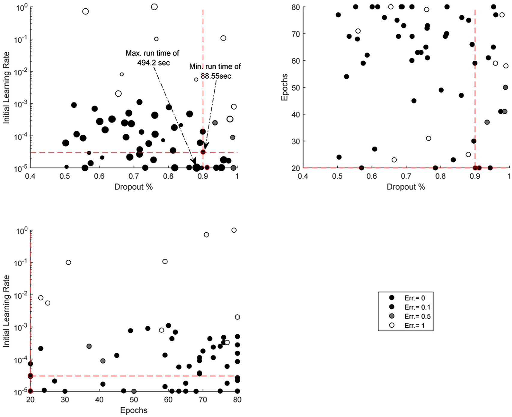
Bayesian optimisation results for hyperparameters of learning rate, maximum number of epochs and dropout probability.
Training and testing process
The common methods of training a neural network algorithm are stochastic gradient descent (SGD) and batch gradient descent methods. In the former, the weights are updated and adjusted immediately after each training round; in the latter, the weights are updated once the error is calculated for the entire training data. While the former converges faster, the number of epochs is considerably higher than the batch method. The combination of these methods is referred to as the mini-batch method, in which the weights are trained for a fixed size of training data. In this study, the mini-batch gradient descent with momentum is used. In comparison to the classic SGD approach, gradient descent with momentum accelerates gradient vectors in the optimal direction, improving the converging speed. This is a very common approach in training a very deep CNN. Further details of gradient descent with momentum can be found elsewhere. 26
To train and test the algorithm, 70% of collected signals are used for training and 30% are held for testing. The latter dataset has not been seen by the algorithm at any point of training. For a machine with an i9-7940x processor, CPU @3.10 GHz and memory of 32 GB, each training round, using the optimised hyperparameters and with a mini-batch size of 5, takes 20 minutes. The following section presents the experimental setup and the result of the training process and performance of the algorithm using the testing dataset.
Experiment setup using model train and bridge
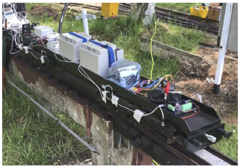
To demonstrate the applicability of the proposed data-driven damage identification approach, a model train is instrumented with six uni-axial accelerometers to detect changes in dynamic characteristics of a model bridge. Figure 4 shows the model train and bridge used for the testing in this study. The model train was driven by a model class 66 locomotive with the total weight of 111.12 kg, followed by a driving trolley with the total weight of 40.63 kg and three additional carriages with respective total weights of 79.1, 77.64 and 40.24 kg. Details of the axle weights and axle spacings for the model train are provided in Figure 4(b). For instrumenting the train, six Isotron 256-100 accelerometers were attached to the body of the front locomotive car. This type of accelerometer uses a built-in low noise microelectronic amplifier which transmits its low impedance voltage output through the same conductor cable that supplies the required current power. Figure 5 demonstrates the sensor placement for the front car.
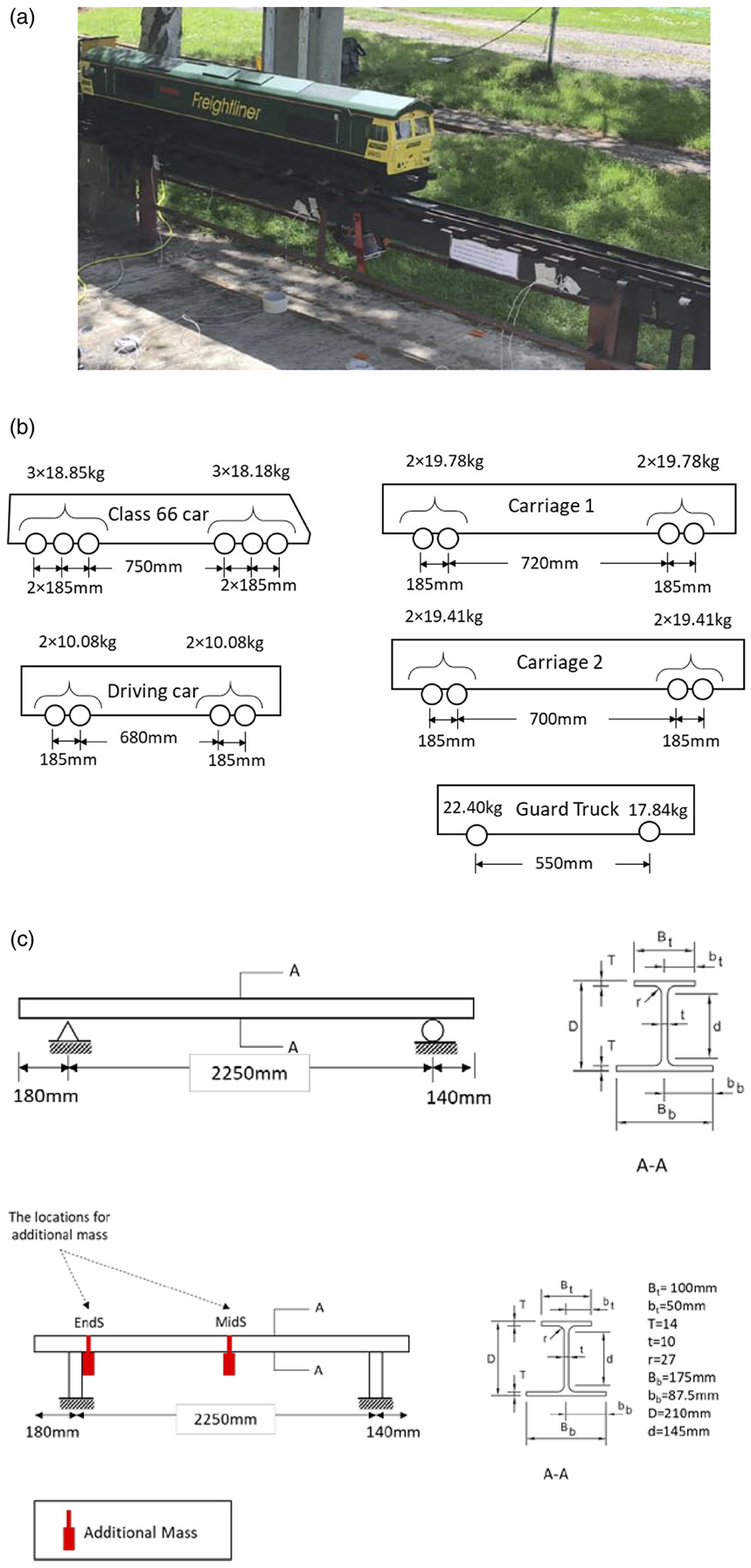
Model bridge and train details: (a) Image of the model train and bridge, (b) model train axle spacings and weights and (c) schematic bridge and its cross-section diagram.
Sensor placement.
The model bridge is a steel asymmetrical I beam of 2.56 m. Figure 4(c) provides details of the cross-section size and support placement in this beam. In order to alter model bridge’s dynamic characteristics, additional weight was added to two different locations on the bridge, mid-span and around the end support. The intensity of the added weight was also changed to create four positive damage scenarios: M1EndS, M1MidS, M2EndS and M2MidS. In this classification, M1 and M2 refer to the addition of 5.5 and 10 kg, respectively and EndS and MidS refer to the location of the additional mass at the end support and mid-span. The additional mass results in a change in vibration characteristics of the structure without damaging the structure. These changes are used as a form of damage indication in this study.
Figure 6 shows the change in frequency content of the bridge following the passage of the model train for the healthy, M1MidS and M2MidS positive damage scenarios, under 4 miles/h travelling speed. As can be seen from the power spectrum diagram, there is not a significant difference in the frequency content of the signals for these three scenarios. The increase in mass is expected to shift the fundamental natural frequencies of the structure however since the magnitude of the added mass in comparison to the mass of the bridge and the model train is relatively low, the shift in frequency is not discernible. To investigate the differences in frequency content, the persistence spectrum is used in Figure 6(c). A persistence spectrum is a form of frequency histogram in power-frequency space, representing the percentage of the time a certain frequency is present in a signal. Figure 6 shows that the additional mass represents a higher persistence in the frequency range of 0.5–0.9 kHz.
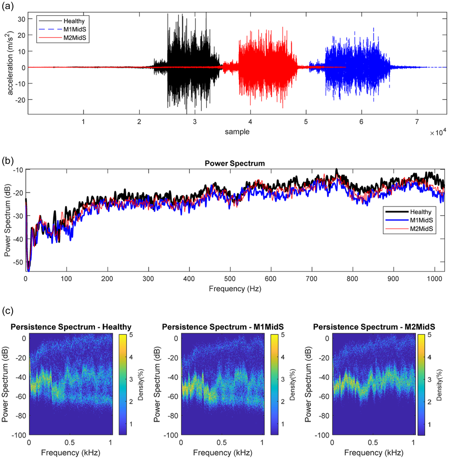
Change in frequency content for a sample of direct measurements: (a) sample of signals, (b) power spectrum and (c) persistence spectrum.
To account for variability in speed in practice, the model train travelled over the bridge at three different speeds of 2, 4 and 6 miles/h. In order to allow sufficient distance to build up the speed, the acceleration signals not only cover the selected model bridge but also measurements over neighbouring bridges. In total, three sets of measurements were collected for the healthy and four positive damage scenarios (i.e. 3 sets of measurement for each sensor and each damage state), resulting in a total number of 90 sets of measurement (6sensors×3speeds×5scenarios) of which 18 represent healthy (benchmark) state and 18 sets of measurements are collected for each positive damaged state.
Figure 7 shows a sample of measured signals under a healthy state and positive damage state of M2MidS. As can be seen from this figure, the signals cannot be compared point-to-point as the length of the signals are different and the speed of the vehicle is only an average speed; hence, there is a slight variability in the length of the signal. In this study, these signals are utilised without the prior knowledge of the actual start point of the bridge as even with the most accurate GPS systems, identifying the exact location of a bridge can be inaccurate in practice. This further highlights the power of the proposed approach in this study. As can be seen from the persistence spectrum, the difference between the signals for healthy and positive damage scenario is quite difficult to discern; however, a subtle change in power density in the region on 0.5–0.8 kHz can be observed.
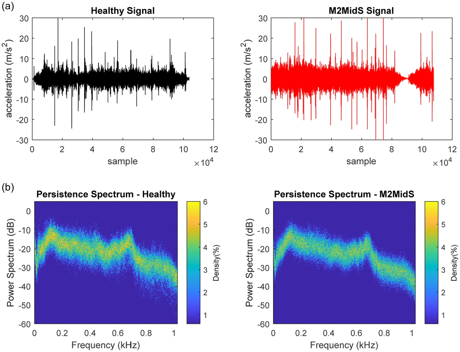
A sample of train-borne acceleration measurements and corresponding persistence spectrum.
In the context of vibration-based damage identification systems, raw signals are rarely used as damage sensitive features. These signals are often processed to produce sensitive features to a wide range of damage signatures. Among different techniques, continuous and discreet wavelet transform, 27 empirical mode decomposition,28–30 power spectrum and frequency spectrum14,31 have been widely used as damage sensitive features. In addition to signal processing techniques, statistical analysis and principal component analysis are also often employed in order to reduce and optimise the dimension of the extracted features.32,33
For the purpose of this study, a wide range of signal processing techniques are explored to identify the best damage sensitive feature. Following this investigation, it was concluded that in order to take advantage of the power of 2D CNN, time–frequency analyses offer powerful images with more distinguishing features to classify train-borne acceleration signals. Among different approaches, the time–frequency spectrogram of the signals is found to provide the best high-level damage sensitive feature. A spectrogram is the squared magnitude of short-time Fourier transform, which itself represents the evolution of frequency content of the signal over time. In this approach, Fourier transform is applied to short segments of original signals as shown in equation (6)
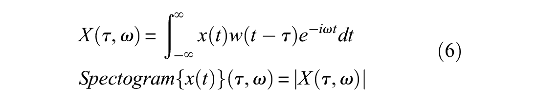
where
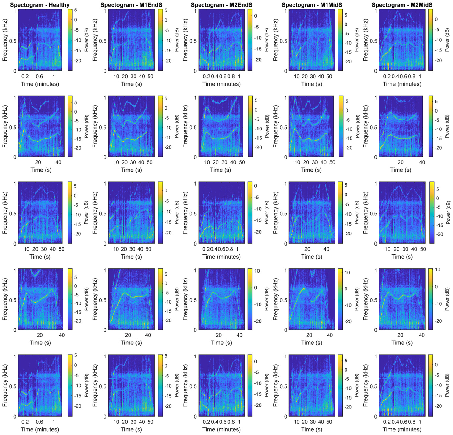
A sample of time–frequency power spectrogram analysis for benchmark and four positive damage scenarios.
The time–frequency spectrogram of each signal was then stored as RGB 274×274×3 images to be used as input in the adapted GoogLeNet learning body. Figure 9 shows a sample of this image for healthy and positive damage scenario of M2MidS.
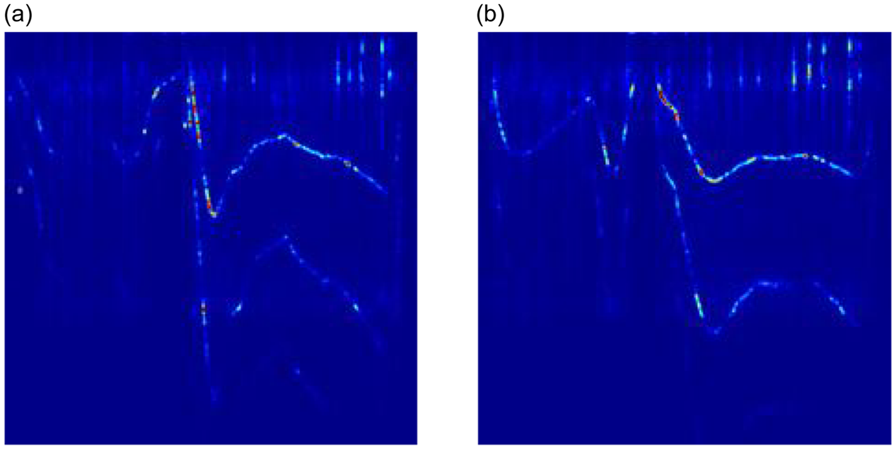
A sample of input images: (a) Healthy spectrogram and (b) M2MidS spectrogram.
Results and discussion
Using the optimised hyperparameters and 70% of all healthy and damage scenario spectrogram images, the adapted GoogLeNet is trained first to detect damage and then classify damage. Once the algorithm is trained, its performance is tested on 30% of the remaining images, which have not been shown to the algorithm before. In the detection exercise, the output is divided into two binary classes of healthy and positive damage, whereas in classification (also referred as localisation), the output consists of five classes of healthy and four positive damage scenarios.
Figure 10 shows the confusion matrix for the classification task for both testing and training datasets. The confusion matrix represents the prediction results categorised as true-positive, true-negative, false-positive and false-negative. In binary classification (i.e. damage detection), true-positive and true-negative represent the correct predictions of healthy and positive damage state, while false-positive and false-negative are the incorrect predictions of healthy and positive damage state.
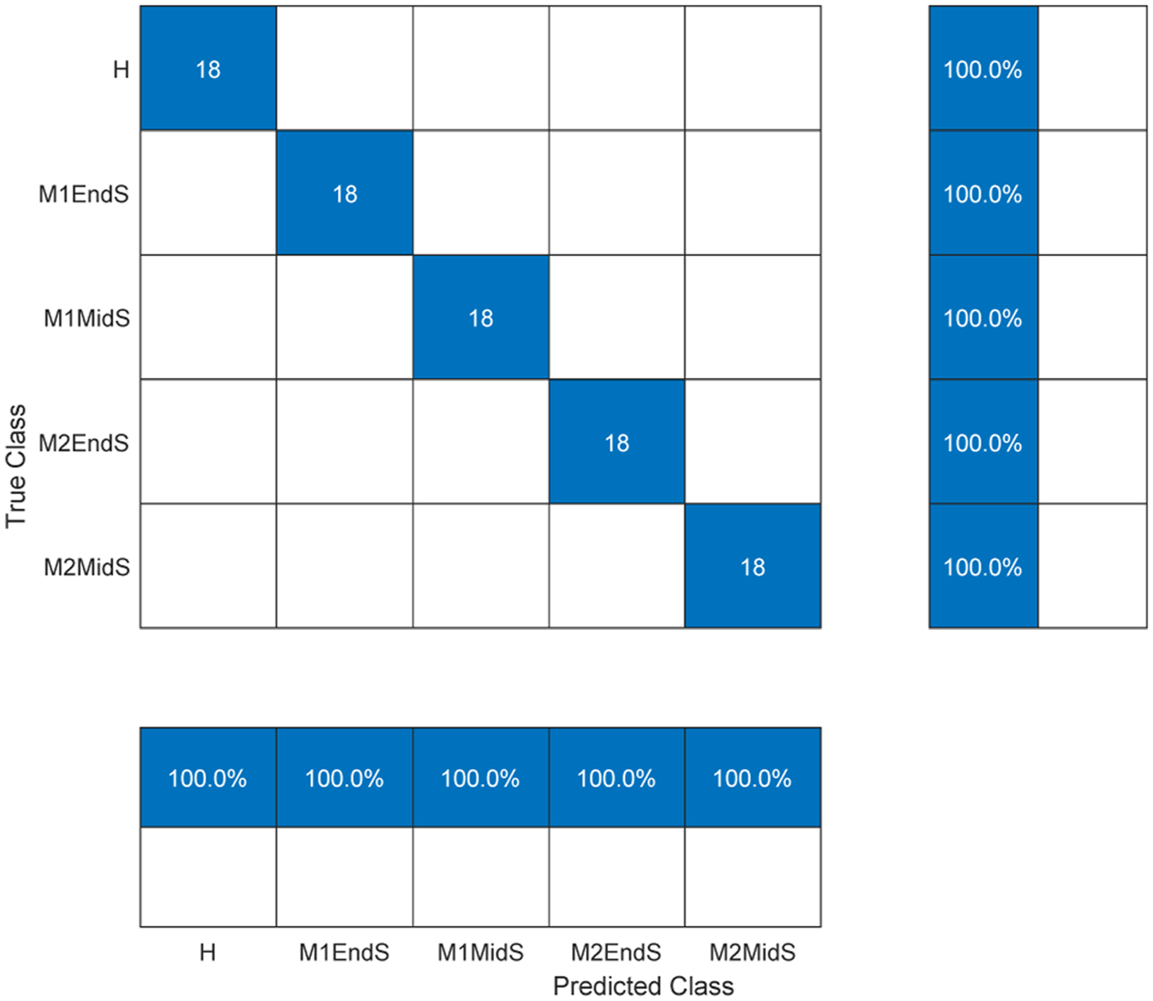
Prediction accuracy of damage detection algorithm for different levels of damage at different locations.
As can be seen from this figure, the trained algorithm is capable of detecting and classifying the damage with 100% accuracy. In comparison to the results in the literature, the proposed method eliminates the need for any specialist pre-processing of the input signals and is the first investigation to consider the operational condition. This approach also offers great accuracy in comparison to reported methods in the study conducted by Locke et al. 14 and Malekjafarian et al. 13 This highlights the power of the proposed algorithm in distinguishing small changes in structural dynamic characteristics without the need for direct instrumentation.
To better demonstrate how the algorithm distinguishes between these different classes, the gradient-weighted class activation mapping 34 is used here. In this approach, the most discriminating pixels of the input image are identified by searching through features extracted by convolutional layers. This process can be expressed using equation (6)
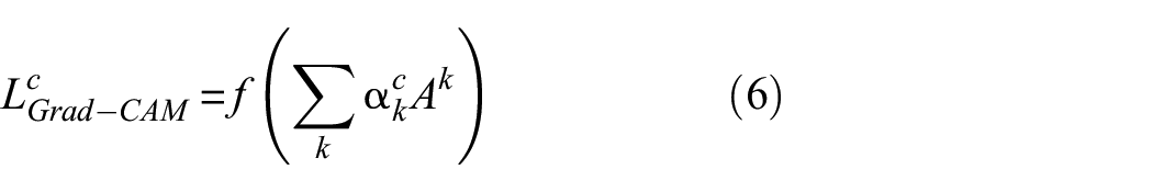
where
in which
An example of discriminating cues from spectrogram images - original image on the left and the corresponding highlighted sensitive zones on the right column: (a) and (b) healthy state, (c) and (d) M1EndS, (e) and (f) M2EndS, (g) and (h) M1MidS and (i) and (j) M2MidS.
Generally, in a deep algorithm, earlier layers of a learning body focus on low-level features such as edges and colours, while deeper layers provide high-level features such as discriminating regions in an image by combining features in earlier layers. To demonstrate the difference between earlier and deeper layers, Figure 12 shows the normalised and scaled activation images corresponding to the maximum activating channel for the first pooling layer (i.e. max pool layer 3×3) and last inception layer (i.e. inception (5b)). In this figure, white pixels represent strong positive activation while black pixels show negative activation. It can be seen that the white pixels are in line with the observations from Figures 6, 8 and 11.
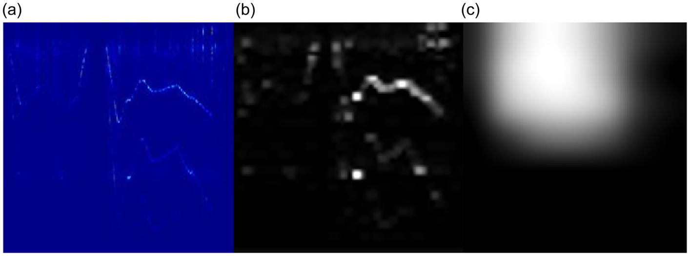
An example of discriminating cues from spectrogram images: (a) Original image for M2MidS, (b) activating features in max pool layer 333 and (c) activating features in inception (5b).
To further investigate the power of deeper layers in the learning body of the trained CNN, the t-distributed stochastic neighbour embedding method is used. 35 In this method, pairwise distances between high-dimensional points are calculated to create a similarity matrix for each point. This is then used to create a low-dimensional set of data and the process is iteratively repeated to update the low-dimensional points with the objective of minimising the Kullback–Leibler divergence between a Gaussian distribution in high-dimensional space and a t-distribution in the low-dimensional space. 35 Figure 13 shows the clustering power of the earlier pooling layer to the final convolution layer and softmax layer. As can be seen from this figure, high-level features have much stronger clustering power in comparison to low-level features in earlier layers.
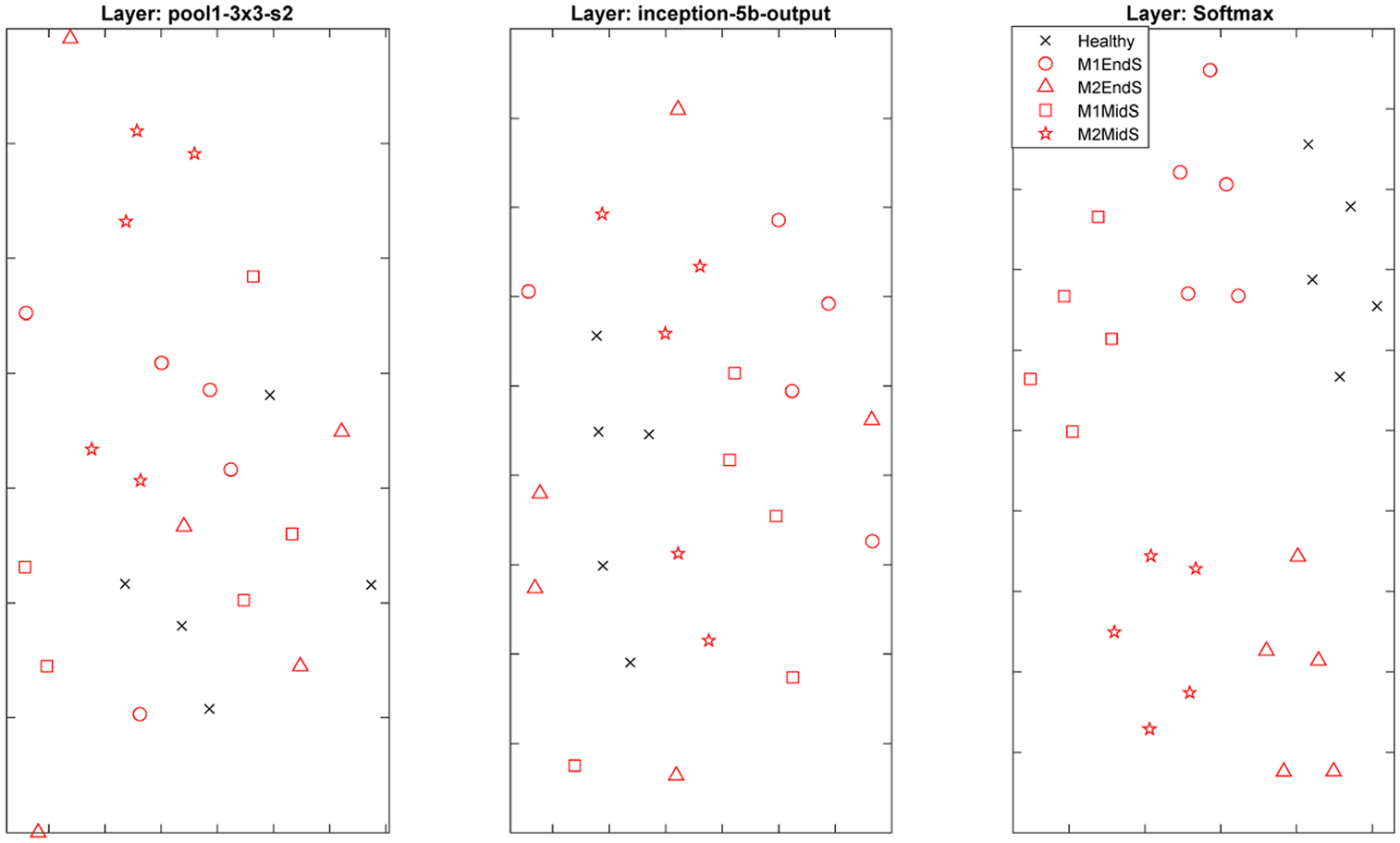
An example of network behaviour from the first pooling activation layer to final softmax activations.
Recommendations for future work
This study presents the first scaled experimental proof-of-concept for a data-driven drive-by damage identification system. While the collected measurements are affected by the operational conditions (varying speed), a systematic investigation of varying environmental and operational conditions is needed to better understand how different contaminating factors could mask signatures for different damage locations and intensities.
This study builds a foundation for follow up studies investigating the capabilities of the algorithm for different structural forms, materials, damage classes and different vehicle configurations. The proposed approach demonstrates the feasibility of the algorithm in detecting and classifying damage (first and second levels of damage identification). The next step will be to expand the application to higher levels of damage identification, that is, prediction of the remaining lifetime.
The current structure of the input data uses the spectrogram of raw train-borne acceleration signals from six accelerations only, with the assumption that additional supporting information such as vehicle speed and rail irregularities does not exist, to demonstrate the feasibility of the approach in the absence of such information. However, incorporating such information in the architecture of the input structure may further improve the accuracy of the algorithm in practice. Further investigations are required to explore how this information can be placed in the input data and how this can impact accuracy.
Conclusion
This study presents the application of a two-dimensional CNN algorithm in developing a data-driven damage identification system to detect and classify damage using train-borne measurements only. The transfer learning technique is used to exploit the power of a pre-trained deep neural network and re-purpose the algorithm for damage identification purposes. The potential of CNN algorithms is widely exploited in computer vision applications. Although their implementation in SHM tasks is growing rapidly, their application in vibration-based damage detection systems has been very limited.
In this study, a well-known pre-trained CNN entitled GoogLeNet is adapted to detect and classify damage signatures in a bridge. The algorithm’s hyperparameters are fine-tuned using Bayesian optimisation to ensure model robustness without significant compromise on computational cost. A proof-of-concept experiment is designed to demonstrate the feasibility of the proposed approach in a scaled operational environment. For this purpose, a model train is instrumented with accelerometers, travelling over a model bridge at varying speeds. To emulate the changes in dynamic characteristics of a bridge due to damage, four positive damage scenarios are considered in which additional weights with two intensities are added to the mid-span and end of span of the model bridge. It is shown that spectrogram of raw train-borne acceleration can be used as a damage-sensitive feature, capable of discriminating small changes in dynamic characteristics of a structure. The labelled spectrogram images are used to generate the input spectrum images without any additional pre-processing. The algorithm is then trained and validated using 70% of train-borne measurements and tested using the remaining 30% of unseen measured signals.
The results show a remarkable accuracy of the algorithm in detecting and classifying temporary changes for the considered damage scenarios. Further details on the behaviour of inner layers of the algorithm show that activating higher and lower level features identified in the learning body is consistent with the sensitive zones observed in direct bridge measurements. The results demonstrate the great potential of the proposed method in transforming the current practices in visual inspection and direct monitoring.
Footnotes
Acknowledgements
The author thanks Mr Bryan Finch at Guildford Model Engineering Society for his great help and support in facilitating the scaled proof-of-concept experiment. The author also thanks Dr Suryakanta Biswal for his valuable help in the train and bridge instrumentation process.
Funding
The author(s) received no financial support for the research, authorship, and/or publication of this article.