Sage Journals: Discover world-class research

Abstract

The degradation of roads is an expensive problem: in the United Kingdom alone, £27 billion was spent on road repairs between 2013 and 2019. One potential cost-saver is the early, non-destructive detection of faults. There are many available techniques, each with its own benefits and drawbacks. This paper builds upon the successful processing of magnetic flux leakage (MFL) data by echo state networks (ESNs) for damage diagnostics, by augmenting ESNs with the depth of concrete cover as part of a data fusion approach. This fusion-based ESN outperformed a number of non-fusion ESN comparators and a previously used analytical technique. Additionally, the fusion ESN had an optimal threshold value whose standard deviation was three times smaller than that of the nearest alternative technique, potentially prompting a move towards automated defect detection in ‘real-world’ applications.

Keywords

Echo state networks non-destructive testing magnetic flux leakage cover depth steel-reinforced concrete heterogeneous data fusion signal processing damage detection

Introduction

The degradation of transport infrastructure is an international problem. For example, in 2013, a UK HM Treasury policy paper stated that £10 billion would need to be spent on repairs to roads by 2021.¹ In the most recent statistics released by the Department for Transport, the actual figure for England alone up to 2019 was £26,651,000,000.² Deteriorating infrastructure in the United States is expected to cost the US economy an average of 400,000 jobs per year up until 2040.³

The detection of steel reinforcing bar (rebar) defects is a particular area of difficulty. For example, the major concrete repair project which began in 2017 on the UK’s busy M5 motorway saw significant delays due to an underestimation of the extent of the damage to the rebar: 6000 repairs were required, 4500 more than the original estimate.⁴ Vanniamparambil et al.⁵ noted that many different modalities of sensor are available for the assessment of the various aspects of structural integrity, but there is no single monitoring technique that can provide a comprehensive picture of the state of a structure. Instead, they concluded that a data fusion approach should be developed in order to better detect deterioration signs, locate weak regions and assess damage severity.

Based on past success in detecting rebar defects with the artificial intelligence of echo state networks (ESNs), this paper proposes an approach to detecting defects that uses ESNs to fuse heterogeneous data obtained by the electromagnetic anomaly detector (EMAD) technique, which is a form of magnetic flux leakage (MFL), and data regarding the depth of concrete cover. This is the first time that these two modalities have been combined, and has been able to improve the detection of defects.

The EMAD technique is a non-destructive testing (NDT) approach that uses remanent magnetism (RM) and MFL in order to detect breaks in rebars. The idea of using RM in this context was first proposed by Scheel and Hillemeier⁶ in 1997. The EMAD technique, meanwhile, has been developed at Keele University over a number of years, and details of the method were first published in 2006.⁷ It has since been the subject of further publications, which have seen the application of computational intelligence (CI) approaches to the automated analysis of data captured by the technique, most recently in 2018.⁸ The EMAD technique has been applied commercially in order to assess structures such as bridges, car parks and dual carriageways, with data processed by using an analytical technique (AT) (introduced fully in the Analytical Technique section). This requires a skilled engineer to set a threshold on an arbitrary scale, based on their insight and judgement. This, in turn, requires time, and so an automated ESN data fusion approach was conceived in order to capture some of this expertise and move towards greater automation. The Magnetic Flux Leakage section describes briefly the theory behind the EMAD technique and how it is applied practically.

Statement of Problem

An example of some EMAD data, featuring two defects at known locations, can be seen in Figure 1. The two defects can be recognised by the characteristic shape of the plot-lines, as the recorded Z component rises to reach a peak at the centre of the defect, while the recorded X component exhibits a slope with a negative gradient at this point.

Figure 1.

A typical set of EMAD data, with the Z axis data shown beneath the X axis data. The characteristic signatures of the two defects present in this particular dataset are highlighted.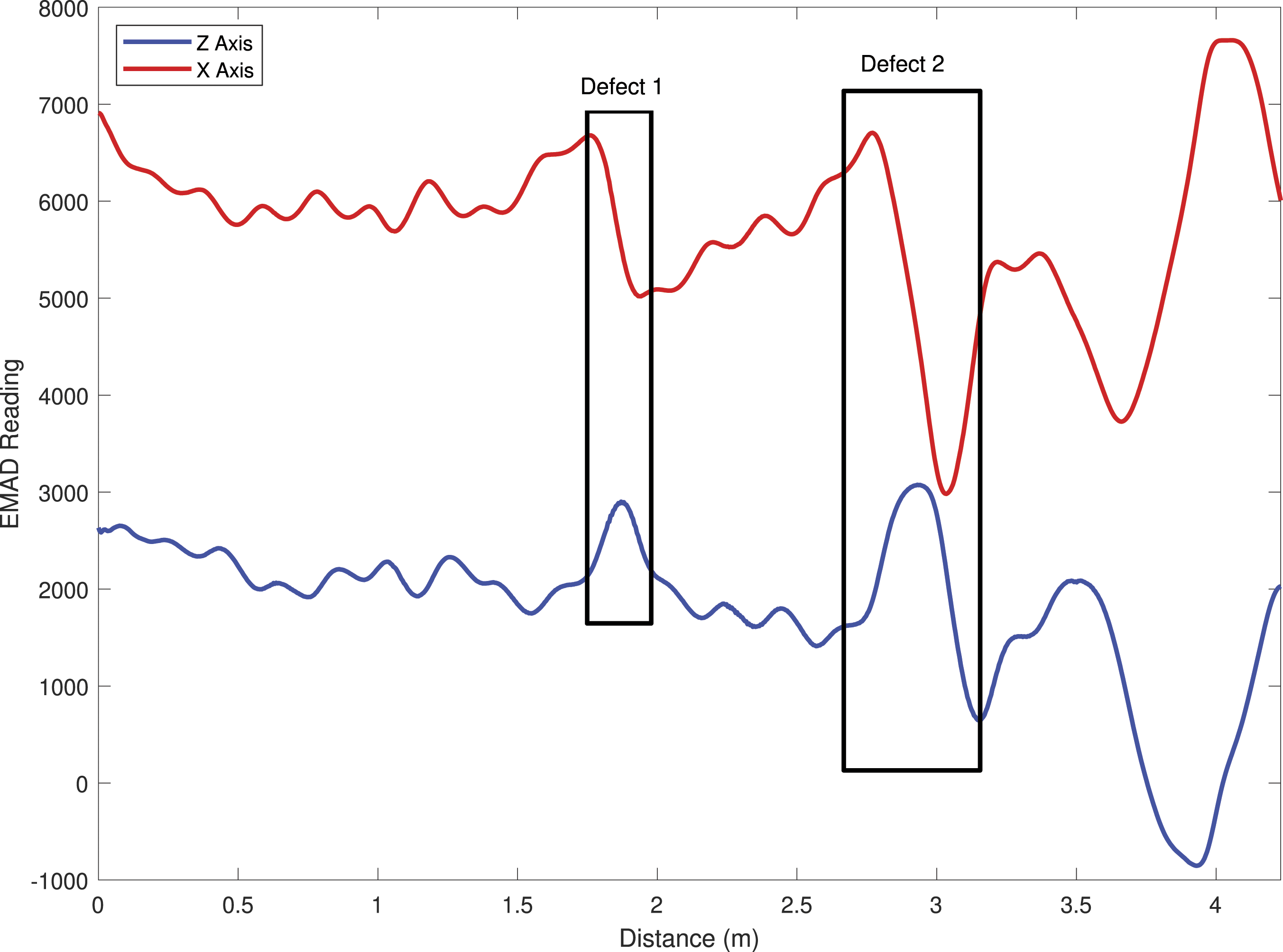

There are a few possible confounding signals that are inherent in using MFL to detect defects, evidence of which can also be seen in Figure 1. The most prominent example of this is the ‘end effect’, where a large magnetic pole is created at the ends of the rebar scan lines, more so at one end than the other. Here, this can be seen from 3.5 m onwards. End effects are usually much larger than defect signals, but the two can still be easily confused. Also, in the case of some rebar meshes, a small amount of flux leakage is observed at points where the longitudinal and transverse rebars cross over, leading to a ‘ripple’ effect. This effect can be seen in the range 0–2.5 m. Since corrosion in rebar is usually local – typically, there may be a few centimetres of corrosion and a much longer section of clean steel⁹ – one of the key challenges with any defect detection technique is the accurate and precise location of such potential defects.

The AT that has previously been used for processing EMAD data in commercial surveys could produce similar outputs for both a minor magnetic anomaly scanned at a close distance, and a major defect recorded from further away. In a ‘real-world’ scenario, this could lead to significant defects being ignored, or repairs taking place to address only minor anomalies. A more effective data processing approach should be able to identify defects clearly and unambiguously, preferably without the need for further interpretation by experts in order to set appropriate output threshold values.

Based on the previous success enjoyed by ESNs in comparison to the AT when presented with EMAD data obtained from a constant cover depth,¹⁰ a data fusion approach that utilises both cover depth and the unique properties of ESNs is presented in this paper. The effectiveness of this data fusion approach, in terms of both defect detection and ‘real-world’ applicability, is demonstrated by comparing the data fusion ESN to a number of non-fusion alternative ESN architectures and the AT. The novel contribution of this paper is the application of an ESN-based data fusion approach that combines MFL data with cover depth data. While the fusion of heterogeneous data for defect detection in rebar has seen an increase in interest in recent years (see, e.g. Refs. [11–13]), the automated fusion of MFL and cover depth data has not been attempted prior to the current work.

There are two key requirements for a data fusion approach to be successful in this context:

1. Competitive performance across the range of cover depths, such that there is a reasonable expectation that a fusion-based approach will be at least as accurate at detecting defects as the non-fusion approaches across the different cover depths.

2. There should be as little variation in the optimal threshold as possible, so as to reduce the need for expert interpretation of the data and allow for faster interventions.

Point two is possibly less intuitive, but just as significant as point one. In the datasets presented in this paper, the full ground truth defect locations are known, making the task of determining the optimal threshold for the output of each technique relatively straightforward. In a ‘real-world’ setting, the ground truth is unlikely to be known, and so expert analysis of the raw data is usually required to help set this threshold. This usually involves a recommendation to break out the concrete to inspect the rebar at two or more locations in order to calibrate the threshold. If the optimal threshold value is very consistent across all possible cover depths, then that would make the setting of the threshold much easier, and hence, render the technique more readily applicable in the ‘real-world’. In short, high accuracy at the optimal threshold is much less valuable if it is difficult to find that optimal threshold without ground truth data.

Contribution of Paper

Since the AT currently used to analyse EMAD data on site requires intervention by a trained engineer to set the threshold for defect detection, one of the aims of using CI is to automate that process. However, the use of ESNs, or any other form of artificial neural network (ANN), leads to an automated optimum range for the threshold after training, rather than a single value. This leads to considerable arbitrariness in the setting of the threshold for the network to be used in the field if that range is too large. Use of EMAD data alone does, indeed, leave the optimum threshold range not closely defined. In this work, a fusion-based ESN architecture was applied to the detection of rebar defects using a combination of EMAD and cover depth data. In doing so, it both outperformed a number of non-fusion ESN comparators and a previously used analytical technique in the detection of defects per se, all of which used EMAD data alone. Moreover, it was also found that the fusion ESN had an optimal threshold value whose standard deviation was three times smaller than that of the nearest alternative technique, implying a large advantage over other techniques in terms of real-world applicability. This is the first time that cover depth data has been automatically fused with any kind of MFL data in this context, while it is also the first time that ESNs have been used for data fusion in NDT.

Structure of Paper

This paper is structured as follows. The data gathering and data processing methodologies are reported in the Material and Methods section. Here, the data fusion approach is described, followed by an explanation of the AT and two non-fusion ESN comparators. This is followed by the Results and Discussion section, where the experimental outcomes are discussed, while concluding remarks are offered in the Conclusions section.

Material and methods

Magnetic Flux Leakage

This subsection briefly discusses the procedure for performing a survey using the EMAD technique. A more detailed account of the physical and mathematical principles behind MFL can be found in Sawade and Krause.¹⁴

At the beginning of any EMAD scan, the rebars are magnetised by passing an electromagnet along their length. In accordance with the principles of RM, the rebars then remain in a magnetised state. A typical scan using the EMAD technique will not be of one single bar, but several bars arranged in a mesh. In this case, each bar in the mesh must be magnetised. After magnetisation has been completed, the EMAD probe is then scanned along the surface of the concrete to detect defects. The probe contains a triaxial magnetic sensor which measures the three Cartesian components of the magnetic flux, X, Y and Z. The probe is passed over each rebar and records data every 4.71 mm. The Z axis readings for the flux give the magnitude of the component of the flux leakage in the direction of the scan and the X axis readings provide the component normal to the concrete surface. Although the Y axis data are recorded, they are rarely used in practice.

Echo State Networks

ESNs are a form of recurrent neural network (RNN) introduced in the early 2000s and were designed to be able to process time-series data. Furthermore, they are efficient to train and have been successfully applied in similar case studies in the past (see, e.g. Refs. 15 and 16). They were developed with an engineering perspective in mind, and have proved to be more effective than traditional ANN methods at predicting complex time-series data, while also having a much shorter training time.¹⁷ For example, ESNs have been shown to provide good performance and significantly superior training times in comparison to state-of-the-art long short-term memory networks (LSTMs),^18,19 temporal expression tree classifiers and genetic programming ensembles.²⁰ One of the most useful aspects of ESNs is their ability to recall past inputs through the presence of a short-term memory, which can be influenced by a careful tuning of the network parameters.²¹ These ESN architecture features make them a particularly good fit for the kind of heterogeneous data fusion required here. In recent times, ESNs have been used for a wide range of applications, such as traffic management,²² soil temperature modelling,²³ power grid voltage insulator damage classification,²⁴ waterflood performance prediction²⁵ and wind speed forecasting.²⁶

The general ESN architecture has three principal features. The first of these is an input layer of neurons which, via a fully connected weight matrix, projects into the second feature, a typically much larger, high dimensional ‘kernel’ of sparsely interconnected reservoir neurons. Each of the reservoir neurons is in turn fully connected to a layer of output neurons. A schematic diagram of this architecture can be seen in Figure 2.

Figure 2.

A typical ESN topology. Only the weights between the reservoir neurons and the output units are trained.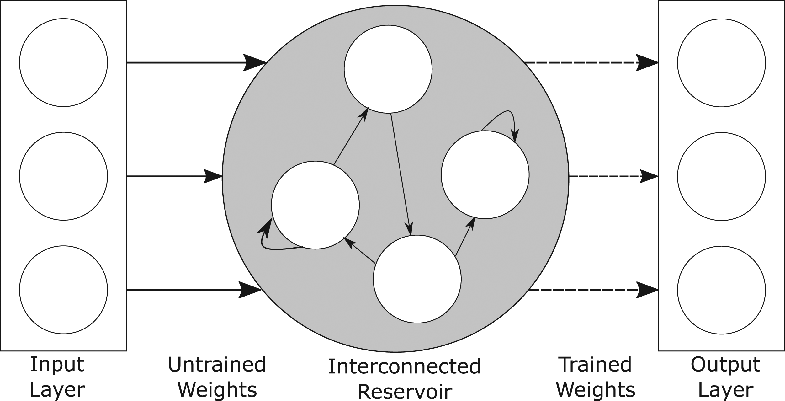

Since their inception in 2001, ESNs have become popular due to their modelling capacity, modelling accuracy, biologically plausible recurrence, extensibility and ability to overcome the vanishing gradient problems traditionally associated with gradient descent RNN training procedures.²⁷ This is achieved by keeping most of the weighted connections between neurons unchanged during training, in contrast to other leading ANN approaches (including deep learning long short-term memory networks), which require all of these connections to be trained. For ESNs, only the weighted connections between the reservoir neurons and the output neurons are trained; all other weighted connections are randomly generated at network initialisation and left unchanged throughout. Ridge regression²⁸ has been found to be a good approach to training the weighted connections between the reservoir and output neurons.^29–31 In this work, ESNs were implemented using the Reservoir Computing Toolbox for MATLAB.³²

The carefully controlled degree of recurrence in the reservoir gives ESNs a key characteristic: the echo state property.²¹ This is simply defined as the state of the ESN, S, at any time, t, depending not only on the input at t, but also on the input at all previous time steps. The state of the network at t is governed by an echo function, E, which maps the history of the vector of network inputs, u, to the current network state, as shown in equation (1)^33,34

S (t) = E (\dots, u (t - 1), u (t))

(1)

Rather than having a fixed memory length, the sparsity of the reservoir allows for a more flexible short-term memory. Although ESN reservoir neurons were initially simple additive units with sigmoid activation functions, most ESN reservoirs now use leaky integrator neurons, first proposed by Jaeger in 2007.³⁵ The activation of a leaky integrator neuron in an ESN reservoir is given by equation (2)³⁶

x (t) = f ((1 - δ) x (t - 1) + δ (W_{i n p}^{r e s} u (t) + W_{r e s}^{r e s} x (t - 1)))

(2)

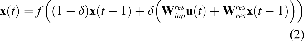
In equation (2), f is the activation function (typically tanh) $W_{i n p}^{r e s}$ is the input layer to reservoir weight matrix, x(t) is the vector of the activations of the reservoir neurons at t, $W_{r e s}^{r e s}$ is the reservoir weight matrix (drawn randomly from a Z distribution) and δ is the leak rate, which determines the extent to which ESN reservoir neurons’ activations decrease over a period of time.

In all, four separate techniques were used:

• Fusion ESN: An ESN that combined X and Z component data from the EMAD with cover depth information and a bias input unit.

• ESN _GD: An ESN that used the X and Z component data from the EMAD and a bias input unit. This was subject to the same training regime as the Fusion ESN but without any cover depth information available.

• ESN _DS: Seven different ESNs trained to use the X and Z component data at specific cover depths, that is, ESN_42.5 trained to detect defects for cover depths of 42.5 mm, ESN₂₈₉ trained to detect defects for cover depths of 289 mm etc.

• The AT: A procedural algorithm that has been developed to exploit the characteristic defect signatures in the X and Z axis data from the EMAD and which has seen commercial use alongside expert interpretation.

These are detailed more fully in the Data Processing section.

Data Gathering

To test the ability of ESNs to fuse EMAD and cover depth data, datasets were obtained in which systematic changes to the cover depth were made. At this point, it is worth re-emphasising one of the key considerations in this study: any real-world survey would require a counter-plot threshold to be applied to a data processing model output before a usable contour plot could be produced. In this academic study where ground truth data is available, we can determine each technique’s optimal threshold based on the proportion of known defects detected on each thresholded contour plot. However, any technique which requires fewer candidate thresholds to be used while delivering state-of-the-art accuracy could reasonably be considered superior, or at least ’more useful’, in day to day usage.

Data fusion testing mesh

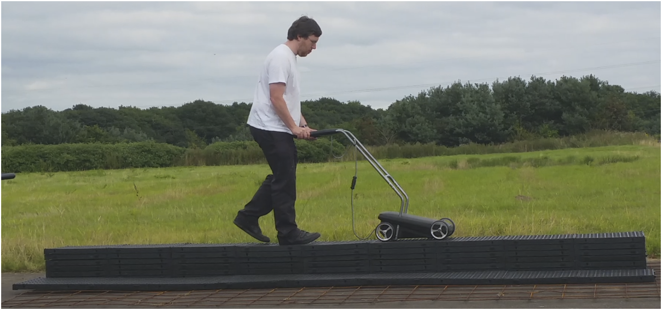
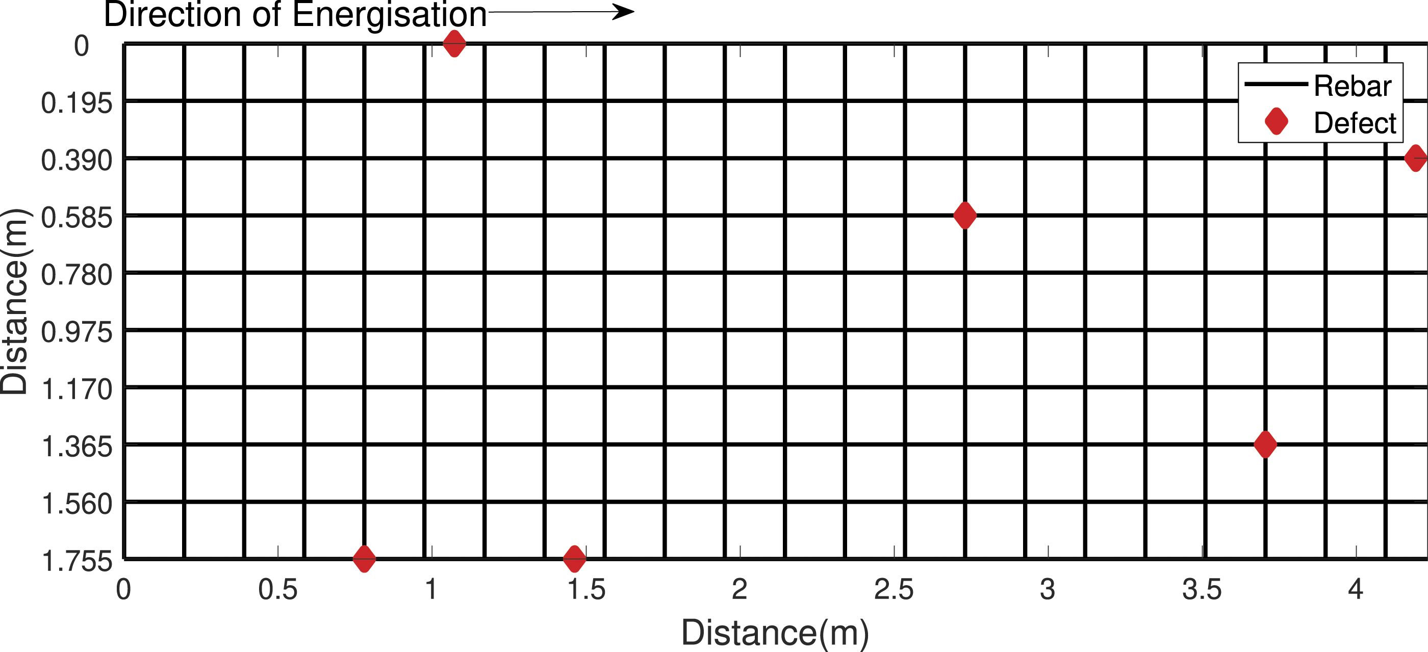
A steel reinforcing mesh was set up for the purpose of obtaining datasets that could be used for data fusion. Seven different concrete cover depths were simulated by using a stack of plastic grids to increase the elevation of the EMAD above the mesh during seven different scans. The covers depths ranged from 42 mm to 289 mm, the limit at which the EMAD probe can detect anomalies. The experimental set-up of this mesh, with a cover depth of 289 mm for just one portion of the mesh, can be seen in Figure 3. The grids were moved across the mesh to access different sections in turn. Figure 4 shows a scan being performed at a cover depth of 251 mm. A schematic view of the mesh’s layout, along with the ground truth location of six manually inserted breaks, is given in Figure 5.

Figure 3.

The data fusion testing mesh in-situ, with a simulated cover depth of 289 mm set up.

Figure 4.

An EMAD scan being carried out with a simulated cover depth of 251 mm.

Figure 5.

The layout of the data fusion testing mesh. Lines represent rebar, while diamonds represent ground truth defect locations.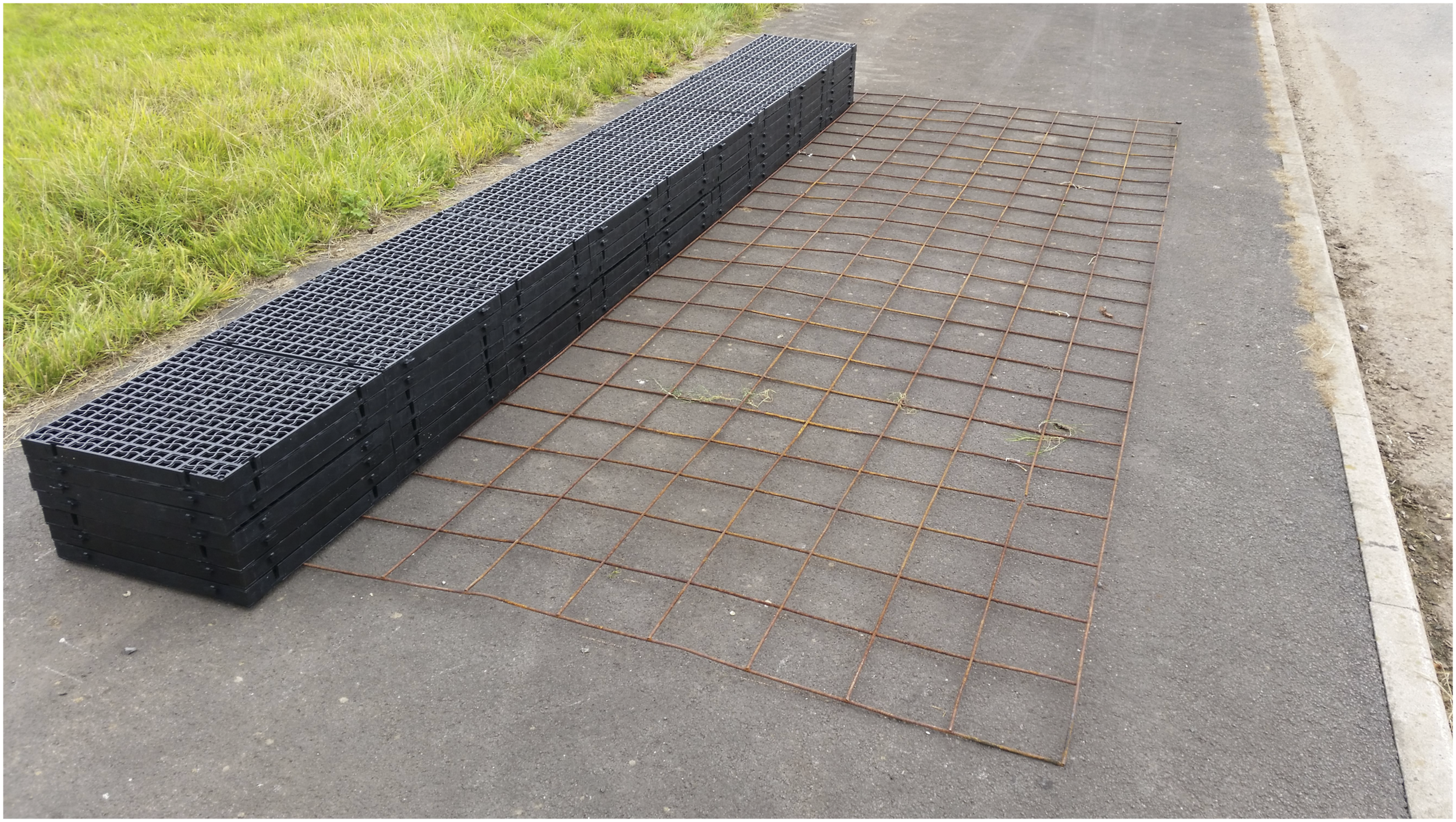

Seven different cover depths were simulated by using plastic grids to increase the elevation of the EMAD above the mesh during seven different scans. The cover depths ranged from 40 mm to 280 mm, the limit at which the EMAD probe can detect anomalies.

Recording MFL data

The first part of the data gathering process was to magnetise the mesh. This was done by passing the energiser over each longitudinal rebar in the mesh at a cover depth of 42.5 mm in the direction indicated in Figure 5. The rebars were each magnetised in turn from right to left, such that the rebar located at 1.755 m in Figure 5 was the first to be energised and the rebar located at 0 m the last. After magnetisation of the whole mesh, each line was then scanned by the EMAD at seven different cover depths: 42.5 ± 0.5 mm, 85.0 ± 0.5 mm, 124 ± 0.5 mm, 165 ± 0.5 mm, 205 ± 0.5 mm, 251 ± 0.5 mm and 289 ± 0.5 mm. Each scan was performed twice – once each by two different EMAD probes – so as to create two separate datasets. All of the data were normalised between +1 and −1 before being presented to the ESN variants considered here. The end result was two EMAD datasets, with 70 scan lines in each. These are henceforth referred to as datasets C1 and C2.

Although these datasets reflected the same physical reality, they were separately obtained by different EMAD probes, and therefore, varied slightly depending on each device’s noise characteristics and calibration. However, in order to fully develop and assess the generalisation capabilities of the data processing techniques employed, a further dataset obtained from an entirely different rebar mesh, C3, was also used in training. This mesh was encased in concrete and the ground truth condition was known. The mesh then underwent multiple cycles of magnetisation in different directions, before then being magnetised in the same direction as the data fusion testing mesh and surveyed to produce a fourth dataset, C4, which was used for testing.

Recording Concrete Cover

Recording the concrete cover presented a challenge, since the maximum cover depth that can be recorded by commercially available covermeters is just 200 mm, 80 mm short of the EMAD’s maximum scanning depth. While this would be less of an issue in the ‘real-world’, where the concrete cover should be well within the range of the covermeter, it meant that commercially available covermeters were not appropriate for the systematic experimental work that was intended here, since it is important for the ESN to be able to model the full range of signals that could be obtained by the EMAD probe. Consequently, the cover depth was entered into the data file as a third parameter which, in this case, was simply recorded for each point in the scan as the height to which the probe had been raised above the mesh.

In order to reflect further the margin of error seen in data obtained by a covermeter, Gaussian white noise equivalent to variation in the range ± 2 mm was added to the data.

Summary of datasets: In summary, the four datasets used in this study were as follows:

• C1: data taken from an EMAD device with varying cover depth, used for training.

• C2: data taken from a different EMAD device with varying cover depth, used for testing.

• C3: data taken from a different, noisier mesh, used for training the Fusion ESN and ESN_GD.

• C4: data taken from the noisier mesh after a series of different energisation cycles, used for testing.

Data Processing

A data fusion methodology was formulated and applied to the recorded EMAD and cover depth data. Since each data point in each dataset was registered with a corresponding cover depth, ESNs can simply accept the cover depth as an additional input. In addition, some alternative ESN approaches were designed for comparison with this data fusion approach. These were ESN_GD (‘General Depth’), which was trained on data obtained from all cover depths, and ESN_DS (‘Depth Specific’), a collection of ESNs that were trained to work on data obtained at specific cover depths. The details of these are recorded below.

Fusion Approach

The data fusion approach that was used here was a relatively simple one. An ESN was created with three inputs: X axis component of the magnetic flux, Z axis component of the magnetic flux and cover depth. This ESN had one output unit, which was trained to give a value of −1 when no defect was present and +1 when a defect was present. An additional ‘bias’ input unit was also used, since it was found that repeatedly feeding the network with an input of +1 improved performance. There is some precedent for this in the literature, with Jaeger suggesting that such ‘bias’ input units improve training effectiveness when the mean value of the desired output is not zero, by increasing the variability of individual neurons’ dynamics.^33,34

Datasets C1 and C3 were used for training, which was performed using ridge regression, and then, C2 and C4 were used as unseen testing datasets. This meant that the ESN was trained on data from seven different cover depths, including lines both with and without defects.

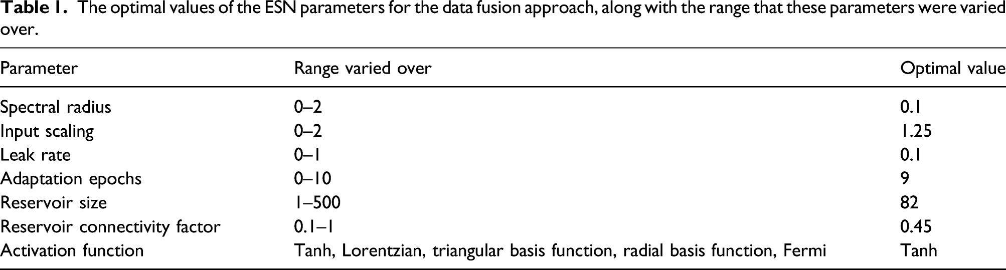
Before the performance of the data fusion ESN approach could be measured, the best performing ESN configuration had to be found. The parameters that were varied, the range over which they were varied and the optimal values that were found can be seen in Table 1.

Table 1.

The optimal values of the ESN parameters for the data fusion approach, along with the range that these parameters were varied over.

Parameter	Range varied over	Optimal value
Spectral radius	0–2	0.1
Input scaling	0–2	1.25
Leak rate	0–1	0.1
Adaptation epochs	0–10	9
Reservoir size	1–500	82
Reservoir connectivity factor	0.1–1	0.45
Activation function	Tanh, Lorentzian, triangular basis function, radial basis function, Fermi	Tanh

Once the best performing ESN configuration had been found, 500 ESNs were trained and their average performance on the testing dataset recorded. This was done in order to account for the fact that an ESN’s weights are randomly generated at initialisation. Different approaches to analysing the data were then used for comparison with this data fusion technique, and these are detailed in the subsections below.

Analytical Technique

In past commercial use, EMAD data were processed using a combination of expert interpretation and a procedural algorithm, referred to here as the AT. This AT has been described previously,¹⁰ and so, a lengthy explanation is not required here. A summary of the AT is given by equation (3)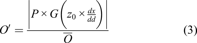

O^{'} = \frac{| P \times G (z_{0} \times \frac{d x}{d d}) |}{\bar{O}}

(3)

For any given data point, the value of the Z component data, z ₀, is multiplied by the magnitude of the slope in the X component data at that point, $\frac{d x}{d d}$ , where the second d in the denominator denotes the distance along the scan. A Gaussian smoothing function, G is then applied to this. The smoothed function is multiplied by the peak-to-peak amplitude between the nearest peak and trough that the data point sits between. Finally, the output is divided by the mean output for the entire length of the scan, $\bar{O}$ , which acts as a scaling factor.

Since it is the usual technique for processing EMAD data, the AT was applied to C2 and C4. If the data fusion approach could not outperform the AT, then it would not have shown any improvement over this existing method.

Depth-Specific ESN (ESNDS)

One alternative approach to the problem of different cover is to have a suite of pre-trained ESNs, each of which has been specially trained to process data recorded at a specific cover depth. In the ‘real-world’, cover measurements could be taken and then the most appropriate ESN selected for the recorded cover depth, bearing in mind that in practice cover can vary considerably across a large area of mesh.

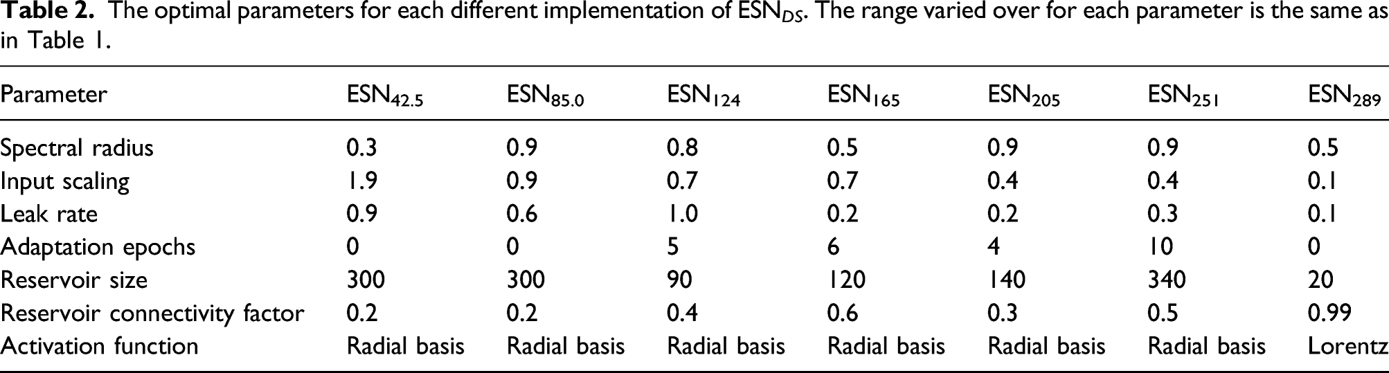
In order to explore this potential scenario, seven separate ESN architectures were trained, one for each different level of simulated cover. As before, 500 ESNs of each configuration were trained and their average testing performance measured. Although there was a relative paucity of training data for these ESNs, the fact that these depth-specific ESNs would only ever be exposed to data recorded at one cover depth compensates for this. Each ESN had two input units (X axis and Z axis components), and a single output unit, which was trained using ridge regression to give values of −1 for no defect and +1 for a defect. The addition of a bias input unit, as used in the fusion ESN and ESN_GD, did not yield improved performance during training, and so was not included in the final model. Dataset C2 was used as an unseen testing dataset, while the ESN trained on data obtained at a cover depth of 42.5 mm was also tested on C4, where the cover depth was approximately 41 mm.

The best performing ESN parameters that were determined for each ESN_DS are given in Table 2. The lack of a consistent pattern of changes in each parameter reflects one of the potential problems with this type of approach. Having access to such a small amount of training data, which is an inevitable consequence of using data obtained only at specific depths, could expose the depth-specific ESNs to overtraining and poor generalisation.

Table 2.

The optimal parameters for each different implementation of ESN_DS. The range varied over for each parameter is the same as in Table 1.

Parameter	ESN_42.5	ESN_85.0	ESN₁₂₄	ESN₁₆₅	ESN₂₀₅	ESN₂₅₁	ESN₂₈₉
Spectral radius	0.3	0.9	0.8	0.5	0.9	0.9	0.5
Input scaling	1.9	0.9	0.7	0.7	0.4	0.4	0.1
Leak rate	0.9	0.6	1.0	0.2	0.2	0.3	0.1
Adaptation epochs	0	0	5	6	4	10	0
Reservoir size	300	300	90	120	140	340	20
Reservoir connectivity factor	0.2	0.2	0.4	0.6	0.3	0.5	0.99
Activation function	Radial basis	Radial basis	Radial basis	Radial basis	Radial basis	Radial basis	Lorentz

General Depth ESN (ESNGD)

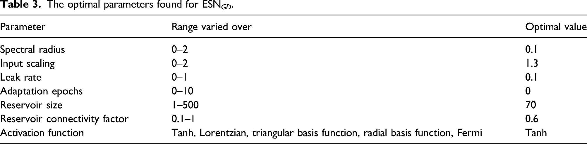
A further alternate approach to the problem of different cover depths that does not involve the fusion of data is to train a single ESN on EMAD data from all cover depths, without providing any information about the cover depth itself. This ‘general depth’ approach led to ESN_GD, which was trained on the entirety of C1. Since it was exposed to defect signals recorded at a range of cover depths, it was expected to be able to detect the presence of defects at any depth. Again, the ESN_GD networks were trained on dataset C1 and C3 with an output unit that would give a value of +1 for a defect and −1 for no defect. The network had three input units, one each for the X and Z components and one which supplied a constant bias value of ‘+1’. 500 ESNs were trained using this topology and then presented with C2 and C4 as unseen testing datasets. The overall average performance of these 500 ESNs was then used for comparison with the other techniques.

The optimal parameters that were found for ESN_GD after a grid search are given in Table 3.

Table 3.

The optimal parameters found for ESN_GD.

Parameter	Range varied over	Optimal value
Spectral radius	0–2	0.1
Input scaling	0–2	1.3
Leak rate	0–1	0.1
Adaptation epochs	0–10	0
Reservoir size	1–500	70
Reservoir connectivity factor	0.1–1	0.6
Activation function	Tanh, Lorentzian, triangular basis function, radial basis function, Fermi	Tanh

Performance Measures

All of the data processing approaches were trained using datasets C1 and C3, and tested using datasets C2 and C4. Since this is a two-class (‘defect’ and ‘no defect’) problem, performance was assessed using a Receiver Operator Characteristic (ROC) curve.

The area covered underneath this curve, referred to as the area under curve (AUC), is equivalent to the probability that a classifier will rank a randomly chosen positive instance higher than a randomly chosen negative instance.³⁷ In machine learning, the AUC has been found to be a better tool for the analysis of two-class classifier performance than a simple calculation of classifier accuracy^38,39 and has previously been used for assessing performance in NDT.⁴⁰ In the ‘real-world’, the processed EMAD data are normally presented on a thresholded contour plot, so an evaluation method that considers performance at different thresholds is particularly useful. The average AUC for the ESN approaches was, therefore, compared to the AUC for the AT on both of the unseen test datasets.

One practical consideration for the use of any technique in the ‘real-world’ is the consistency of the optimal threshold, which can be found by determining the point on the ROC curve that had the smallest Euclidean distance to the point that would represent perfect classification. When the ground truth is known, as in this case, finding the threshold that produces the clearest contour plots is trivial. However, the ground truth is not usually known, meaning that expert analysis is often required to select the best threshold. If the calculated threshold is consistent across different datasets, then expert analysis is not as important. For each technique, the optimal threshold was calculated and recorded at each different cover depth. A smaller standard deviation of the optimal threshold at each different cover depth would indicate smaller variation in optimal threshold values at different cover depths, and would suggest that the technique would rely less on costly and time-consuming expert interpretation.

Results and Discussion

Results

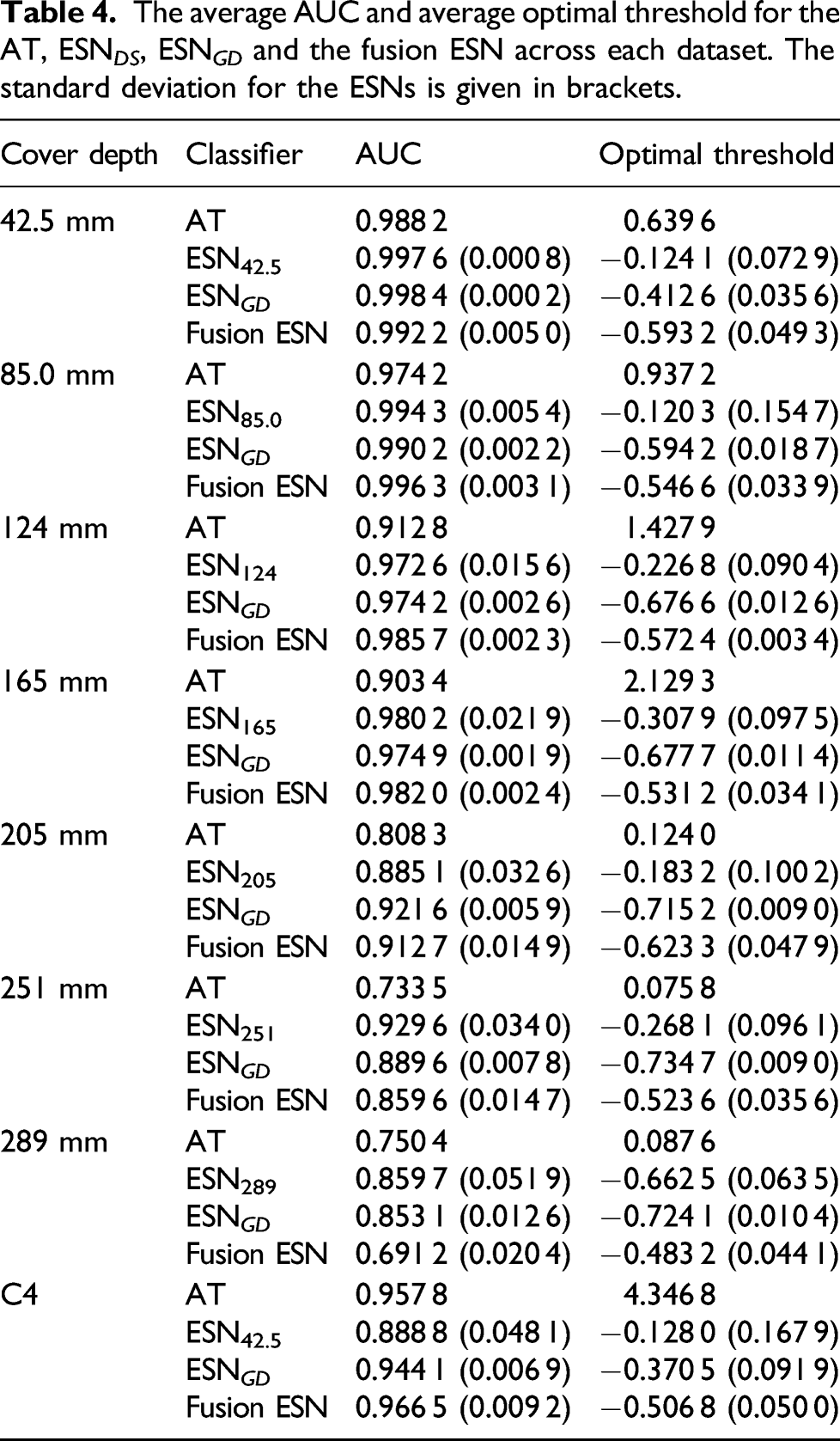
Table 4 shows the results at each different cover depth. The standard deviation for the average optimal thresholds at each depth, meanwhile, is given in Table 5. Figure 6 shows ROC curves at each cover depth for examples of each of the data processing approaches. For each approach, the exact classifier depicted was the one whose performance was closest to the overall average performance.

Table 4.

The average AUC and average optimal threshold for the AT, ESN_DS, ESN_GD and the fusion ESN across each dataset. The standard deviation for the ESNs is given in brackets.

Cover depth	Classifier	AUC	Optimal threshold
42.5 mm	AT	0.988 2	0.639 6
	ESN_42.5	0.997 6 (0.000 8)	−0.124 1 (0.072 9)
	ESN_GD	0.998 4 (0.000 2)	−0.412 6 (0.035 6)
	Fusion ESN	0.992 2 (0.005 0)	−0.593 2 (0.049 3)
85.0 mm	AT	0.974 2	0.937 2
	ESN_85.0	0.994 3 (0.005 4)	−0.120 3 (0.154 7)
	ESN_GD	0.990 2 (0.002 2)	−0.594 2 (0.018 7)
	Fusion ESN	0.996 3 (0.003 1)	−0.546 6 (0.033 9)
124 mm	AT	0.912 8	1.427 9
	ESN₁₂₄	0.972 6 (0.015 6)	−0.226 8 (0.090 4)
	ESN_GD	0.974 2 (0.002 6)	−0.676 6 (0.012 6)
	Fusion ESN	0.985 7 (0.002 3)	−0.572 4 (0.003 4)
165 mm	AT	0.903 4	2.129 3
	ESN₁₆₅	0.980 2 (0.021 9)	−0.307 9 (0.097 5)
	ESN_GD	0.974 9 (0.001 9)	−0.677 7 (0.011 4)
	Fusion ESN	0.982 0 (0.002 4)	−0.531 2 (0.034 1)
205 mm	AT	0.808 3	0.124 0
	ESN₂₀₅	0.885 1 (0.032 6)	−0.183 2 (0.100 2)
	ESN_GD	0.921 6 (0.005 9)	−0.715 2 (0.009 0)
	Fusion ESN	0.912 7 (0.014 9)	−0.623 3 (0.047 9)
251 mm	AT	0.733 5	0.075 8
	ESN₂₅₁	0.929 6 (0.034 0)	−0.268 1 (0.096 1)
	ESN_GD	0.889 6 (0.007 8)	−0.734 7 (0.009 0)
	Fusion ESN	0.859 6 (0.014 7)	−0.523 6 (0.035 6)
289 mm	AT	0.750 4	0.087 6
	ESN₂₈₉	0.859 7 (0.051 9)	−0.662 5 (0.063 5)
	ESN_GD	0.853 1 (0.012 6)	−0.724 1 (0.010 4)
	Fusion ESN	0.691 2 (0.020 4)	−0.483 2 (0.044 1)
C4	AT	0.957 8	4.346 8
	ESN_42.5	0.888 8 (0.048 1)	−0.128 0 (0.167 9)
	ESN_GD	0.944 1 (0.006 9)	−0.370 5 (0.091 9)
	Fusion ESN	0.966 5 (0.009 2)	−0.506 8 (0.050 0)

Table 5.

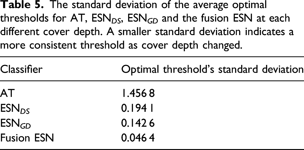
The standard deviation of the average optimal thresholds for AT, ESN_DS, ESN_GD and the fusion ESN at each different cover depth. A smaller standard deviation indicates a more consistent threshold as cover depth changed.

Classifier	Optimal threshold’s standard deviation
AT	1.456 8
ESN_DS	0.194 1
ESN_GD	0.142 6
Fusion ESN	0.046 4

Figure 6.

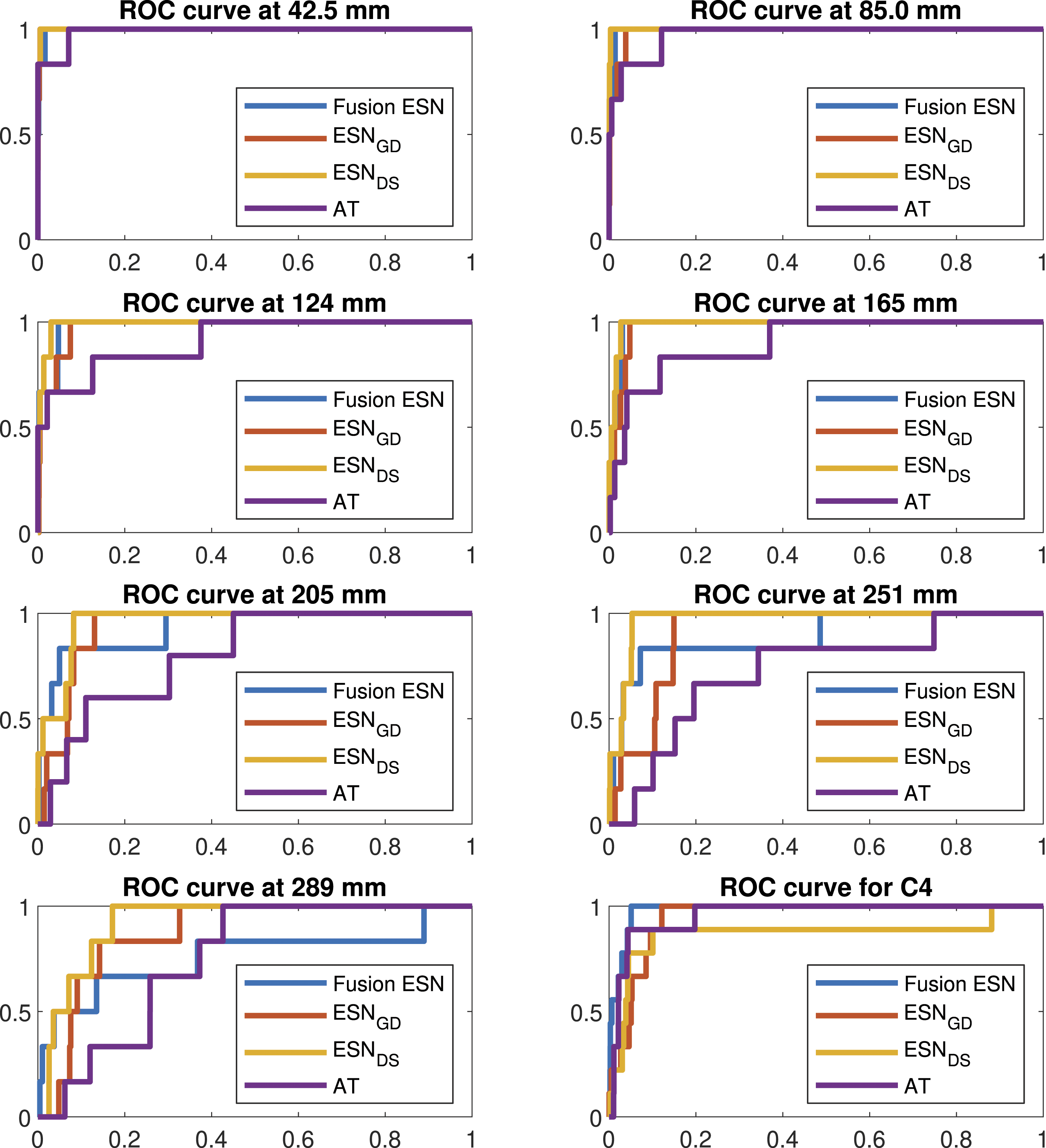
ROC curves for typical examples of each data processing approach at each different cover depth. For each approach, the exact classifier depicted was the one whose performance was closest to the overall average performance. In each of the plots, the false positive rate is given on the x-axis and the true positive rate on the y-axis.

Discussion

It can be seen in Table 4 that the Fusion ESN provided competitive performance at all of the different cover depths with the exclusion of 289 mm, where the signals were so obscure that all of the techniques struggled to produce a usable output. Indeed, the Fusion ESN was the best performing architecture for depths of 85.0 mm, 124 mm, 165 mm and C4. However, the main advantage of using a fusion ESN, and hence, providing the additional context of cover depth, is best seen in Table 5.

In Table 5, it can be seen that the optimal threshold’s standard deviation for the Fusion ESN is three times smaller than the same measure for ESN_GD and over 30 times smaller than for the AT that has previously been applied commercially. A smaller standard deviation indicates that only very small variation in threshold is required to produce an accurate plot of the data from a survey. Indeed, the variation is so small that, regardless of the cover depth, the optimal threshold can almost be left at a constant value, reducing the opportunity for human error.

It is, therefore, possible to envisage how the fusion ESN could be applied in a ‘real-world’ survey. After the initial survey, the average cover depth could be reported to an on-site engineer, who could then select a threshold based on Table 4, but variations around the average depth would then not significantly degrade the analysis. This does not just mean that the fusion ESN can be applied in the ‘real-world’, but that it holds a major advantage over the AT and takes an important step towards more fully automating the analysis process.

In contrast, while the other ESN architectures offered good performance, obtaining this good performance in practice would require an engineer to be able to determine the optimal threshold. This is much more difficult to perform in near real-time on site when the ground truth is not known and may necessitate breaking out sections of rebar in order to get a baseline to help calibrate the threshold. This would add both time and expense to any survey, limiting applicability of the other techniques in ‘real-world’ settings and not guaranteeing that the optimal threshold will actually be found. By simply incorporating cover depth information into a data fusion model, all of this can be avoided.

The ‘real-world’ applicability of the Fusion ESN is also demonstrated through its performance on dataset C4, which was much noisier than C2. This noisy data is potentially more representative of ‘real-world’ surveys and shows that the Fusion ESN is not just capable of working on ‘clean’ data. The ability of the fusion ESN to process usefully this noisy data points to another ‘real-world’ benefit. If none of the techniques were capable of processing the noisier data, then it is possible that the EMAD technique would need to be modified to include additional expensive equipment to provide a saturating field capable of suppressing all conflicting magnetic signals, which would increase the cost of the technique in terms of both time and money.

Taken in combination, all of this suggests that the fusion ESN would be well suited to processing EMAD and covermeter data in the ‘real-world’.

Conclusions

In summary, this paper presented a data fusion approach to the NDT of reinforced concrete that significantly improved upon the AT that has been used hitherto.

The fusion ESN gave competitive AUC values when applied to datasets taken across a range of cover depths. Additionally, the architecture would be a plausible option for systematic application in ‘real-world’ surveys, showing the best performance on noisy data and with the standard deviation of the optimal threshold across all of the cover depths only 0.0464, compared to 0.1426 for the nearest alternative technique. In practice, this would make selection of the optimal threshold and, hence, obtaining the most accurate results much easier in surveys where the ground truth is not known.

Footnotes

Declaration of conflicting interests

The author(s) declared no potential conflicts of interest with respect to the research, authorship, and/or publication of this article.

Funding

The author(s) received no financial support for the research, authorship, and/or publication of this article.

ORCID iD

Adam J Wootton

References

Osborne

Alexander

. Investing in Britain’s Future. Policy Paper Cm 8669. London: HM Treasury and Infrastructure UK, 2013.

UK Government Department for Transport . Maintenance Expenditure by Road Class in England, 2019. URL, https://assets.publishing.service.gov.uk/government/uploads/system/uploads/attachment-data/file/851926/rdc0310.ods

Duncan

Landau

Cutler

, et al. Integrating transportation and economic models to assess impact of infrastructure investment. Transportation Res Rec J Transportation Res Board 2012; 2297: 145–153.

England

Highways

. M5 Junction 1 to 2 Oldbury Viaduct, 2018. URL, https://web.archive.org/web/20181021085724/https://highwaysengland.co.uk/projects/m5-junction-1-to-2-oldbury-viaduct/

Vanniamparambil

Khan

Carmi

, et al. Multiple cross validated sensing system for damage monitoring in civil structural components. In: Structural Health Monitoring 2013: A Roadmap to Intelligent Structures: Proceedings of the Ninth International Workshop on Structural Health Monitoring. Stanford, CA, 10–12 September 2013.

Scheel

Hillemeier

Capacity of the remanent magnetism method to detect fractures of steel in tendons embedded in prestressed concrete. NDT E Int 1997; 30(4): 211–216.

Hocking

North

Wright

, et al. Non-destructive detection of corrosion in steel reinforcement. Concrete Eng 2006; 10: 39–41.

Wootton

Day

Haycock

. Fault detection in steel-reinforced concrete using echo state networks. In: International Joint Conference on Neural Networks (IJCNN), Baltimore, Maryland, 7–11 June 1992, 2018.

Broomfield

. Corrosion of Steel in Concrete: Understanding, Investigation and Repair. London: Taylor & Francis, 1998.

10.

Wootton

. Fusion of Heterogeneous Data in Non-destructive Testing and Structural Health Monitoring Using Echo State Networks, PhD Thesis. Keele: Keele University, 2018.

11.

Haller

Volker

Hartmann

. Machine learning based multi-sensor fusion for the nondestructive testing of corrosion in concrete. In: SMAR 2019 - Fifth Conference on Smart Monitoring, Assessment and Rehabilitation of Civil Structures, Switzerland, 27 – 29 August 2019.

12.

Pashoutani

Zhu

Mazzeo

, et al. Development and Implementation of a Moving Nondestructive Evaluation Platform for Bridge Deck Inspection. University of Nebraska, Nebraska Department of Transportation, 2020. Technical report.

13.

Pfandler

Angst

. Machine Learning Based NDT Data Fusion to Detect Corrosion in Reinforced Concrete Structures with Inspection Data. Onepetro, 2021. CORROSION .

14.

Sawade

Krause

. Magnetic flux leakage (MFL) for the non-destructive evaluation of pre-stressed concrete structures. In: Non-Destructive Evaluation of Reinforced Concrete Structures: Non-Destructive Testing Methods. Oxford: Elsevier; 2010. chapter 11.

15.

Butcher

Day

Austin

, et al. Defect detection in reinforced concrete using random neural architectures. Computer-Aided Civil Infrastructure Eng 2014; 29(3): 191–207.

16.

Wootton

Day

Haycock

. Echo state network applications in structrual health monitoring. In: Proceedings of the 53rd Annual Conference of The British Institute of Non-Destructive Testing, Manchester, UK, 9–11 September 2014. NDT; 2014, pp. 289–300.

17.

Jaeger

Haas

Harnessing nonlinearity: predicting chaotic systems and saving energy in wireless communication. Science 2004; 304(5667): 78–80.

18.

Ramamurthy

Stenzel

Sifa

, et al. Echo state networks for named entity recognition. In: ICANN 2019: Artificial Neural Networks and Machine Learning: Workshop and Special Sessions, Munich, Germany, 17–19 September 2019, pp. 110–120.

19.

Jirak

Tietz

Ali

, et al. Echo state networks and long short-term memory for continuous gesture recognition: a comparative study. Cogn Comput 2020; 1–13.

20.

Lacy

Smith

Lones

. Using echo state networks for classification: a case study in Parkinson’s disease diagnosis. Artif Intelligence Med 2018; 86: 53–59.

21.

Jaeger

. Short Term Memory in Echo State Networks. Fraunhofer Institute for Autonomous Intelligent Systems, 2002. Technical report.

22.

Griesbach

Beggiato

Hoffmann

. Lane change prediction with an echo state network and recurrent neural network in the urban area. IEEE Trans Intell Transportation Syst 2021, 121: 1–7.

23.

Alizamir

Kim

Zounemat-Kermani

, et al. Modelling daily soil temperature by hydro-meteorological data at different depths using a novel data-intelligence model: deep echo state network model. Artif Intelligence Rev 2021; 54: 2863–2890.

24.

Stefenon

Seman

Sopelsa Neto

, et al. Echo state network applied for classification of medium voltage insulators. Int J Electr Power Energy Syst 2022; 134: 107336.

25.

Deng

Pan

. Data-driven proxy model for waterflood performance prediction and optimization using echo state network with teacher forcing in mature fields. J Pet Sci Eng 2021; 197: 107981.

26.

Wang

Tao

. Wind speed forecasting based on variational mode decomposition and improved echo state network. Renew Energy 2021; 164: 729–751.

27.

Lukosevicius

Jaeger

. Reservoir computing approach to recurrent neural network training. Computer Sci Rev 2009; 3(3): 127–149.

28.

Montgomery

Peck

Vining

. Introduction to Linear Regression Analysis. Hoboken, NJ: Wiley, 1982.

29.

Dutoit

Schrauwen

Van Campenhout

, et al. Pruning and regularization in reservoir computing. Neurocomputing 2009; 72: 1534–1546.

30.

Lukosevicius

. A practical guide to applying echo state networks. In: Montavon

Orr

Muller

(eds), Neural Networks: Tricks of the Trade, Lecture Notes in Computer Sci. 2nd ed, Vol. 7700. London: Springer Berlin Heidelberg; 2012, pp. 659–686. chapter 27.

31.

Schrauwen

Verstraeten

Van Campenhout

. An overview of reservoir computing: theory, applications and implementations. In: Proceedings of the 15th European Symposium on Artificial Neural Networks, Belgium, 2–4 October 2020, pp. 471–482.

32.

Verstraeten

Schrauwen

D’Haene

, et al. An experimental unification of reservoir computing methods. Neural Networks 2007; 20(3): 391–403.

33.

Jaeger

. The “Echo State” Approach to Analysing and Training Recurrent Neural Networks - with an Erratum Note. Fraunhofer Institute for Autonomous Intelligent Systems, 2010. Technical report.

34.

Jaeger

. A Tutorial on Training Recurrent Neural Networks, Covering BPPT, RTRL, EKF and the “Echo State Network” Approach. German National Research Center for Information Technology, 2013. Technical report.

35.

Jaeger

Lukoševičius

Popovici

, et al. Optimization and applications of echo state networks with leaky- integrator neurons. Neural Networks 2007; 20(3): 335–352.

36.

Verstraeten

. Reservoir Computing: Computation with Dynamical Systems . Phd thesis. New York: Ghent University, 2009.

37.

Fawcett

. An introduction to ROC analysis. Pattern Recognition Lett 2006; 27(8): 861–874.

38.

Bradley

. The use of the area under the ROC curve in the evaluation of machine learning algorithms. Pattern Recognition 1997; 30(7): 1145–1159.

39.

Jin Huang

Ling

. Using AUC and accuracy in evaluating learning algorithms. IEEE Trans Knowledge Data Eng 2005; 17(3): 299–310.

40.

Jarvis

Cawley

Nagy

. Performance evaluation of a magnetic field measurement NDE technique using a model assisted probability of detection framework. NDT E Int 2017; 91: 61–70.

Heterogeneous data fusion for the improved non-destructive detection of steel-reinforcement defects using echo state networks

Abstract

Keywords

Introduction

Statement of Problem

Contribution of Paper

Structure of Paper

Material and methods

Magnetic Flux Leakage

Echo State Networks

Data Gathering

Data fusion testing mesh

Recording MFL data

Recording Concrete Cover

Data Processing

Fusion Approach

Analytical Technique

Depth-Specific ESN (ESNDS)

General Depth ESN (ESNGD)

Performance Measures

Results and Discussion

Results

Discussion

Conclusions

Footnotes

Declaration of conflicting interests

Funding

ORCID iD

References