Sage Journals: Discover world-class research

Abstract

The increasing demand for civil infrastructures, the aging of existing assets, and the strengthening of safety and liability laws have led to the inclusion of structural health monitoring (SHM) techniques into the structural management process. With the latest developments in the sensors field and computational power, real-scale SHM systems’ deployment has become logistically and economically feasible. However, it is still challenging to perform a quantitative evaluation of the structural condition based on measured data. The paper addresses recent efforts to associate measured observations with an identification of local stiffness reduction as a global parameter for damage onset and growth. It proposes a hybrid methodology for model updating and damage identification. The proposed methodology is built on data feature extraction using the principal component analysis (PCA), finite element (FE) simulation, and Monte Carlo simulation to quantify the extent of local damage of a 60-year-old prestressed concrete bridge. The methodology allows a sensor-specific quantification of the local stiffness reduction and makes it possible to focus succeeding bridge inspection, recalculation, and repair works on these areas. Even more, the monitoring in combination with the FE model and proposed methodology provides continuous information on developing stiffness reduction and the acuteness of rehabilitation measures.

Keywords

Structural health monitoring FBG sensors damage identification model updating prestressed concrete bridges

Introduction

The capability to detect, quantify, and predict damages is the utmost desire of bridge owners to allow an effective and safe structural condition assessment. Traditionally, the practice of periodic visual inspection predominates in maintenance programs throughout the world.¹ However, it is known that visual inspections are insufficient to satisfy the current needs for bridge maintenance.^2,3 Therefore, the inclusion of non-destructive damage detection and structural health monitoring (SHM) techniques into the structural management process has become more and more sought.^4,5

Despite the increasing development of the SHM field, a set of measured data alone is insufficient to precisely assess the actual condition of a structure or detect new damage formation, regardless of how good the sensing technology or how high the data availability.⁶ In this sense, extensive research has been done on the condition assessment of existing bridges based on field tests and numerical analysis in the last three decades.^7–16 Their outcomes highlighted how challenging it could be to perform structural health assessment, mainly due to the difficulty of mathematically describing damage and deterioration processes,¹⁷ and the lack of measurements from real-size damaged structures.¹⁸

SHM strategies can be divided into two categories according to the presence or absence of physics-based numerical models: model-based and data-driven methods.¹⁹ Model-based methods, also known as behavior models, are typically run by optimizing the discrepancy between measured structural responses and FE model predictions in a process called model updating. With a calibrated FE model, existing damages are quantified, new structural changes are identified based on new deviations, and predictions regarding, for example, lifetime expectancy, may be assessed.^20–23 However, FE modeling and updating are time-consuming and comes with a high computational cost. Furthermore, the data interpretation from FE simulations requires user interference, which can jeopardize the detection of structural damage in a timely manner.²⁴

As regards the data-driven methods, also called model-free methods, they dispense information about structural physical responses. Instead, statistical parameters sensitive to structural changes are extracted from a baseline condition using approaches such as the principal component analysis (PCA),²⁵ robust regression analysis (RRA),²⁶ and multi-linear regression (MRL).²⁷ The SHM is then performed by keeping track of those damage features’ changes in time. A deviation in the statistical parameters of a sensor’s time series from the baseline is then deemed as unexpected behavior that could be associated with structural damage.^28–34 The data-driven methods can be performed as post-processing analysis or real-time evaluation and are characterized by their computational simplicity and feasibility to implement online damage detection in SHM of large structures.³⁵ Nonetheless, data-driven methods are usually unable to quantify the identified damages or assess the structural changes that happened before the baseline definition. Therefore, in SHM of existing structures where the detection of new damages and the estimation of the actual structural deterioration level are desired, the advantages of data-driven and model-based methods can be combined to enhance the condition assessment process.³⁶

The acceleration-based modal identification, such as natural frequencies and mode shapes, is far the most common approach in SHM systems.^37,21 Although the acceleration-based sensing can be highly sensitive to damage (e.g., in steel structures or reduced models), natural frequencies lack the spatial resolution to detect local damage in real-scale concrete structures with random damage formation, and mode shapes can be unreliable for large-scale SHM due to excessive measurement noise.²² Cawley,³⁸ for example, reported that a crack with a depth of 1% of the cross-section’s height at the root of a cantilever beam would reflect a reduction of its natural frequency less than 0.1%. Even if 10% of the cross-section were removed, the natural frequency would be less than 1% reduced.

On the other hand, strain sensing is an alternative to measuring the structural response at local and global levels. Many successful applications of electromagnetic point-type strain gauge sensors can be found in SHM systems for steel bridges.^39–45 Nevertheless, traditional electromagnetic point-type strain gauges are too local, thus unsuitable for monitoring inhomogeneous materials such as reinforced and prestressed concrete structures,⁴⁶ where material properties at the macro-level are more indicative of structural behavior. Therefore, strain sensors for SHM purposes of such systems must be insensitive to material discontinuities at the micro- and meso-levels while still delivering reliable measurements at the macro-level.⁴⁷ In other words, it is of interest to measure the behavior of the structure’s resulting material rather than the strain in each of its components (e.g., aggregate, cement paste, and rebar).⁴⁷

In this context, fiber-optic (FO) sensing is an alternative with great potential to fill in the gaps in the condition assessment of large concrete structures.⁶ The distributed and quasi-distributed FO sensors are far the most successful deployed sensing technics in civil structures. The distributed FO sensors (DFOS) based on Rayleigh backscattering, for example, deliver spatial strain or temperature resolution smaller than 1 mm over up to 70 m of continuously measurement length, and Brillouin scattering allow distributed sensing over 200 km with 2-m spatial resolution. DOFS shows outstanding performance, especially on newly constructed structures, where the FO can be embedded or surface mounted to measure the evolution of continuous processes. The exact identification and quantification of crack formation,^48–50 creep and shrinkage assessment,^51,52 prestressing losses control,⁵³ shape assessment,⁵⁴ measure strain and deflection profiles,⁵⁵ and tracking structural changes during construction phase⁵⁶ are examples of SHM of large concrete structures using DOFS. An extensive review of SHM of civil infrastructures using DOFS sensors can be found in.⁵⁷

In contrast, the quasi-distributed FO sensors are characterized by their in-line multiplexing feature. Individual sensors can be connected in series to measure a distributed yet discrete structural length.⁶ The use of fiber Bragg grating (FBG) sensors for quasi-distributed strain measurements dates back to the early 1990s.⁵⁸ However, the sensor’s gauge length was limited back then by the FBG’s length, which ranges few millimeters. With the recent development of long-gauge fiber Bragg grating (LGFBG) FO sensors for structural applications, it is possible to measure the average strain over gauge lengths up to 10-m long,⁵⁹ which can be customized regarding the structure’s size, materials, and static behavior. Therefore, SHM based on quasi-distributed FO sensors can measure the structure’s global and local information,⁴⁷ giving new opportunities for a reliable condition assessment of reinforced and prestressed concrete structures.^34,60–62

Data-driven approaches in combination with FE model simulations have been successfully applied in SHM of bridge structures. Meixedo et al.,¹⁸ for example, proposed a novel unsupervised data-driven methodology to extract damage-sensitive features of train-induced responses using time series analysis and multivariate statistical techniques. The methodology was validated using FE simulations, and a damage indicator was proposed for real-time identification of specific damaged scenarios. Malekzadeh et al.³⁶ introduced an innovative hybrid data interpretation approach using a supervised classification algorithm. The real-time SHM data is analyzed through moving principal component analysis (MPCA) and hypothesis testing. A Monte Carlo simulation is used to simulate and predict structural response and identify predefined damage cases.

Although many successful deployments of SHM on large structures have been presented,⁶³ there is still a need for investigating and developing damage identification and performance assessment of concrete bridges. For most damage identification approaches, the stochastic nature of the damage formation and traffic loading is not considered simultaneously. Therefore, they cannot cope with the random damage scenarios and loading cases of existing highway prestressed bridges, for example, where tendon breaks can occur in any section, and localized stiffness reductions may be inherited back from the construction phase. Moreover, the structural response of statically indeterminate structures such as prestressed bridges is sensitive to stiffness changes. Consequently, a sensor’s abnormal behavior may be caused by damages at its location or by a combination of damages scattered in the structure. Thus, it is paramount that the SHM system of real-size concrete structures is designed with appropriate sensor count, area coverage, and optimized placement to assess the damage distribution correctly. Likewise, a damage detection method should be able to evaluate the sensors’ damage feature sensitivity to stochastic damage scenarios for a reliable damage assessment.

In this sense, this paper’s main contribution is the proposition of a hybrid methodology that combines data-driven and FE model updating approaches to quantify the extend of local damage in terms of stiffness reduction of discretized length segments on an existing prestressed concrete bridge. The dynamic strain data from two parallel quasi-distributed LGFBG sensor arrays—with 27 strain sensors each covering the complete bridge’ length—are analyzed using the PCA to extract statistical parameters describing the static structural response traffic-induced loads. A FE digital twin of the prestressed bridge was implemented to simulate the real sensors’ PCA response during traffic loading. Next, a sensitivity study is set to evaluate the impact of multiple damage scenarios on the extracted PCA features. The model updating is then processed using a Monte Carlo simulation by optimizing the difference between the simulated and measured PCA results. The following innovations were accomplished during this work’s implementation:

• the PCA analysis is performed for categorized heavy vehicles’ crossings rather than time-windowed data series as in MPCA. For that, a clustering algorithm was implemented to identify individual heavy vehicles’ passages from the over 60 thousand recorded crossings and categorize them by the vehicles’ length, number of axles, traveling velocity and direction, and maximal measured strain;

• the development of a Monte Carlo simulation for FE model updating using the PCA sensitivity study to test millions of damage combinations and intensities employing stiffness reduction, but having to run only a few FE simulation in an iterative optimization process;

• the improvement of the damage identification reliability by taking into consideration during the Monte Carlo simulation and optimization not only the eigenvector that represents the first principal component (PC) in the PCA but all the eigenvectors that together explain up to 95% of the static response’s variance;

• to demonstrate that the PCA analysis of a quasi-distributed sensor array covering the structure’s complete length can extract with confidence the driving principles of the structure’s static response during short and individual vehicles’ crossings and eliminate external influences such as environmental and operation variations;

• to show that in statically indeterminate structures, local damages trigger structural behavior changes scattered in the system. Therefore, changes detected by data-driven analysis may be a result of multiple damages positions rather than damage located only at the sensor that presented abnormal behavior.

The proposed methodology is part of a pilot structural health monitoring system developed to access a real-size prestressed concrete bridge in Neckarsulm, Germany. The main goal is to provide real-time structural analysis and robust yet meaningful information to support bridge managers’ decision-making during maintenance. In this paper, the focus is given to detecting and quantifying the extent of local damage in the monitored structure. A novel runtime algorithm for the real-time detection of unexpected structure behavior, such as tendon breaks and excessive crack formation, and more details on the deployed SHM system can be found in Ref. 64.

SHM system in Neckarsulm

Characteristics of the monitored bridge

The monitored structure is a prestressed hollow-core concrete bridge constructed in 1964. The design load class is BK 60 (60 tons wheeled type load), according to DIN 1072. It has three continuous spans without coupling joints with a total length of 57.00 m (17.00 m–23.00 m–17.00 m) and a width of 11.08 m (Figure 1(a) and Figure 1(b)). The superstructure is supported by two linear rocker bearings on the southern abutment, and the northern abutment, by two roller bearings. Like most of the prestressed concrete structures designed until the 1970s in Germany, the bridge was built with prestressing steel types St 145/60 Sigma, KA 141/40, and KA35/10, known for their high vulnerability to corrosion-induced cracking.⁶⁵

Figure 1.

Monitored bridge: (a) longitudinal view of the bridge (dimensions in centimeter); (b) Bridge’s cross-section (dimensions in centimeter); (c) FE model in SOFiSTiK: main deck’s cross-section and prestressing tendons.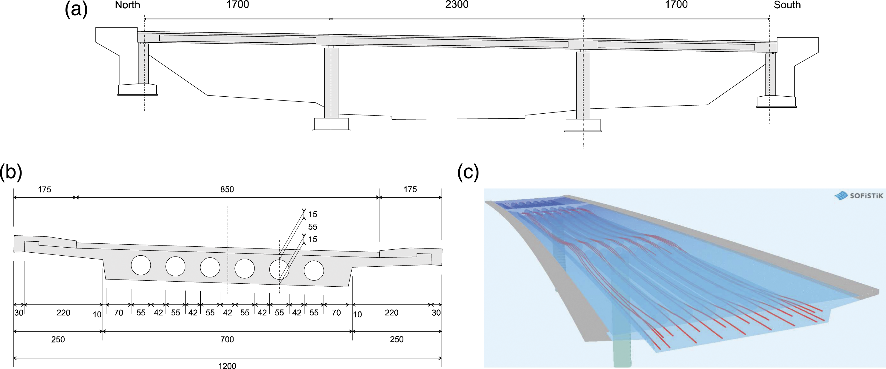

In addition to the high increase in traffic loads compared to the year of construction in 1964 and the corrosion-induced cracking risk, other critical problems may arise due to construction methods and the design standards adopted. Construction failures can already appear during construction caused by misplacement of the hollow-core bodies and difficulties in compacting the surrounding concrete. From the structural point of view, the hollow-core bodies prevent two-axis load transfer. Likewise, shear forces and temperature loads were not considered to the extent that it is deemed necessary from today’s standards when the building was planned. Finally, the hollow-core cannot be examined as part of the building inspection, which means that any damage inside them may not be detected early.

A FE model was build using the SOFiSTiK Bridge Design module. The Bridge Design module has a parametric design tool that optimizes the construction of the structure’s geometry and allows the easy modeling of complex forms, such as curvatures and inclinations, and the prestressing system and tendons’ geometry. The goal was to build a FE model as close as possible to the bridge’s original blueprints. The structure parts were defined as beam elements, with 197 beam elements for the main deck and 50 beam elements for the columns. Figure 1(c) shows an overview of the FE model in SOFiSTiK.

Characteristics of the monitoring system

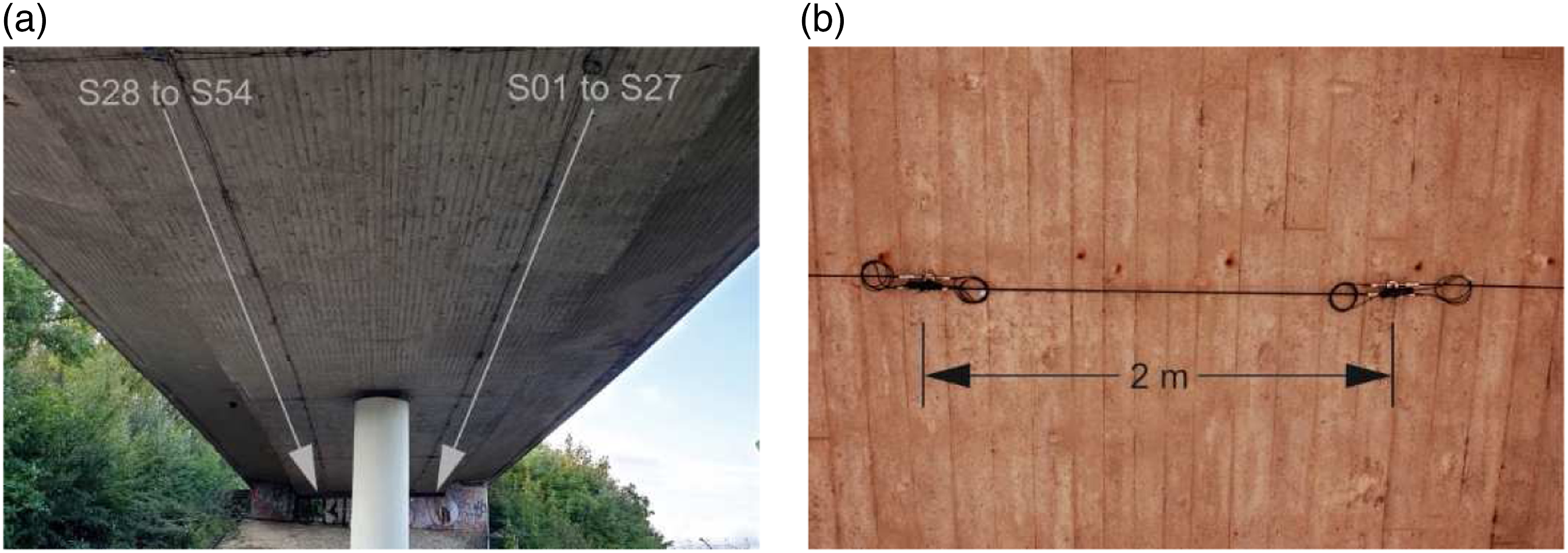
A fiber-optic monitoring system based on long-gauge FBG (LGFBG) sensors was installed to monitor strain and temperature changes of the bridge superstructure continuously. The strain monitoring in the longitudinal direction consists of two parallel measuring lines, each with 27 LGFBG sensors connected in a series along the complete longitudinal length. For every LGFBG strain sensor, an embedded temperature sensor is present for temperature compensation on the FO. A schema of the sensors is given in Figure 2, and overview photos are shown in Figure 3. The LGFBG sensors have a gauge length of 2 m.

Figure 2.

Schema of the sensors’ configuration (bottom view of the superstructure).

Figure 3.

Overview of the bridge and the monitoring system: (a) sensor distribution; (b) an LGFBG sensor with a 2.05 m gauge.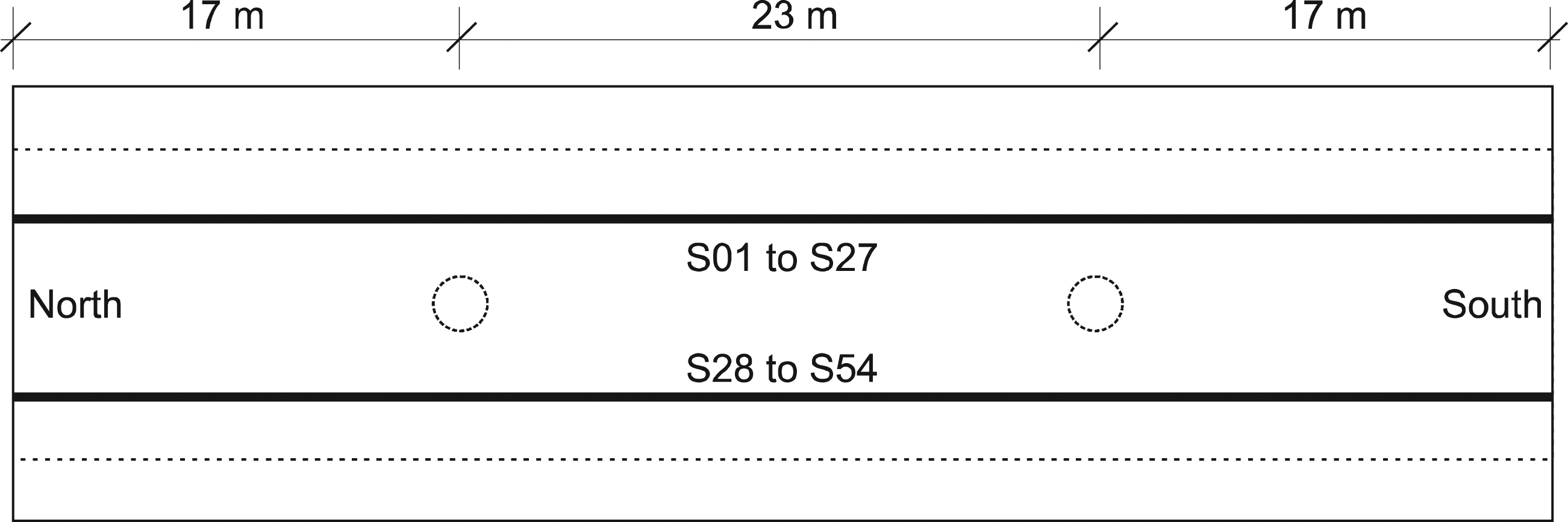

The monitoring system in Neckarsulm has run continuously since November 2019 at a sampling rate of 200 Hz, generating over 70 thousand measurement points per second. The sampling rate was defined to optimize the representation of extreme values such as load peaks during a vehicle’s crossing. Considering that the average travel-ling speed at the bridge is 60 km/h (and there are speed cameras a few meters from the north abutment), a sampling rate of 200 Hz provides an 8-cm measuring step. A comprehensive description of the monitoring system and the data management solution can be found in Ref. 64. More information about the LGFBG sensors and fiber-optic sensing in SHM of concrete structures can be found in Refs. 6 and 66–68.

PCA method

The PCA is a quantitative method to simplify multivariate statistics problems by replacing the original data with a new set of variables containing most of the information, called the principal components.⁶⁹ The principal components have no physical meaning, but they describe the directions that explain a maximal amount of variance, that is, the axes that provide the best angle to see and evaluate the data. The first principal component comprises the axes’ directions that capture each variable’s largest possible variance. The second principal component is another set of axes perpendicular to the first and accounts for the following highest variance. This process continues until the number of calculated principal components equals the number of variables in the original data. The complete set of principal components is a square matrix of order n, where n is the number of variables. However, it is commonplace that the first few principal components explain over 80% of the total variance. Therefore, they can be used to understand the driving forces that generated the original data.⁷⁰

The principal components are constructed by calculating the eigenvectors and eigenvalues of the data’s covariance matrix. The eigenvectors represent the axes’ direction with the most variance, while the eigenvalues are coefficients that give the amount of variance carried by each eigenvector. The principal components are simply the eigenvectors sorted in order of their eigenvalues.⁷¹

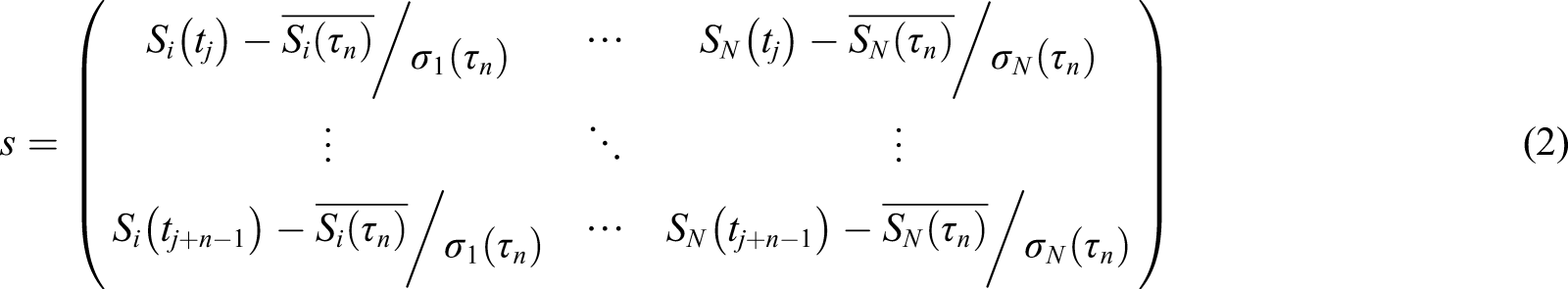
First, a matrix with the strain histories from selected sensors is constructed for the analyzed time window $τ_{n}$ where the result is an N by n matrix

S (τ_{n}) = (\begin{matrix} S_{i} (t_{j}) & \dots & S_{N} (t_{j}) \\ ⋮ & ⋱ & ⋮ \\ S_{i} (t_{j + n - 1}) & \dots & S_{N} (t_{j + n - 1}) \end{matrix}) with i = 1 t o N and n = s i z e (τ_{n})

(1)where N is the number of sensors, j is the first sample in the time window

τ_{n}

, and

n

is the time window’s size in samples. Since the PCA is sensitive to the initial variables’ variances, the resulting matrix must be normalized to assure that they contribute equally to the analysis. Each variable is centered on having a mean of 0 and rescaled to have a standard deviation of 1. The normalized matrix

s

of the strain history is given as

s = (\begin{matrix} \frac{S_{i} (t_{j}) - \bar{S_{i} (τ_{n})}}{σ_{1} (τ_{n})} & \dots & \frac{S_{N} (t_{j}) - \bar{S_{N} (τ_{n})}}{σ_{N} (τ_{n})} \\ ⋮ & ⋱ & ⋮ \\ \frac{S_{i} (t_{j + n - 1}) - \bar{S_{i} (τ_{n})}}{σ_{1} (τ_{n})} & \dots & \frac{S_{N} (t_{j + n - 1}) - \bar{S_{N} (τ_{n})}}{σ_{N} (τ_{n})} \end{matrix})

(2)where

\bar{S_{i} (τ_{n})}

is the mean value and

σ_{1} (τ_{n})

the standard variation for the sensors’ strain history during

τ_{n}

Next, and the covariance matrix

C (τ_{n})

for all measured samples is constructed from the standardized matrix

s

as follows:

C (τ_{n}) = (\begin{matrix} c o v (s_{1}, s_{1}) & \dots & c o v (s_{N}, s_{1}) \\ ⋮ & ⋱ & ⋮ \\ c o v (s_{1}, s_{N}) & \dots & c o v (s_{N}, s_{N}) \end{matrix}) with c o v (s_{p}, s_{q}) = \frac{1}{n - 1} \sum_{k = 1}^{n} (s_{p, k} - μ_{p}) * (s_{q, k} - μ_{q}), p and q = 1 to N

(3)where

μ_{p}

is the mean of the data series

s_{p}

μ_{q}

the mean of the data series

s_{q}

, and * denotes the complex conjugate. Finally, the eigenvalues

λ_{i}

and eigenvectors

Ψ_{i}

of the covariance matrix are obtained by satisfying the equation

[C (τ_{n}) - λ_{i} I] Ψ_{i} = 0

, for i = 1 to N.

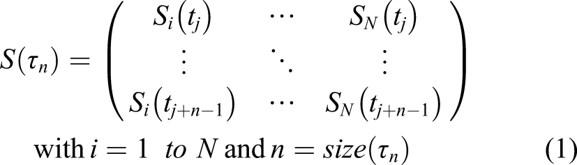
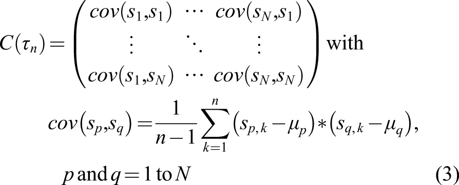
When the eigenvectors are sorted by their eigenvalues in decreasing order, they are arranged in order of significance, resulting in an N × N matrix, also called the principal components (PC) matrix, where N is the number of variables. The first few eigenvectors contain most of the original data variance information, as explained before. They can be used to understand how each variable contributes to the overall behavior and how they interact.

A hybrid methodology for damage identification and quantification

The proposed hybrid methodology is divided into two main tasks: the data-driven tasks (SHM system) and the model-based tasks (FE model). The methodology’s core is the strain feature extraction using the PCA method, which is performed for both the dynamic strain history from the SHM system and the FE model’s simulated results. However, the tasks that precede the PCA analysis in each task have fundamental differences, especially during the data preparation. The SHM system, for example, runs uninterruptedly with a high sampling rate (200 Hz) and is subject to random load cases and environmental and operational variations. Therefore, a clustering algorithm was implemented to extract the sufficiently uniform data to correlate with the simulated FE results. As for the FE model, the damage locations and their intensities are unknown. Hence, a sensitivity analysis together with a Monte Carlo simulation is used to test millions of damage combinations and intensities cases. Figure 4 shows the workflow’s summary with the methodology’s main tasks.

Figure 4.

A hybrid methodology for structural identification and model updating.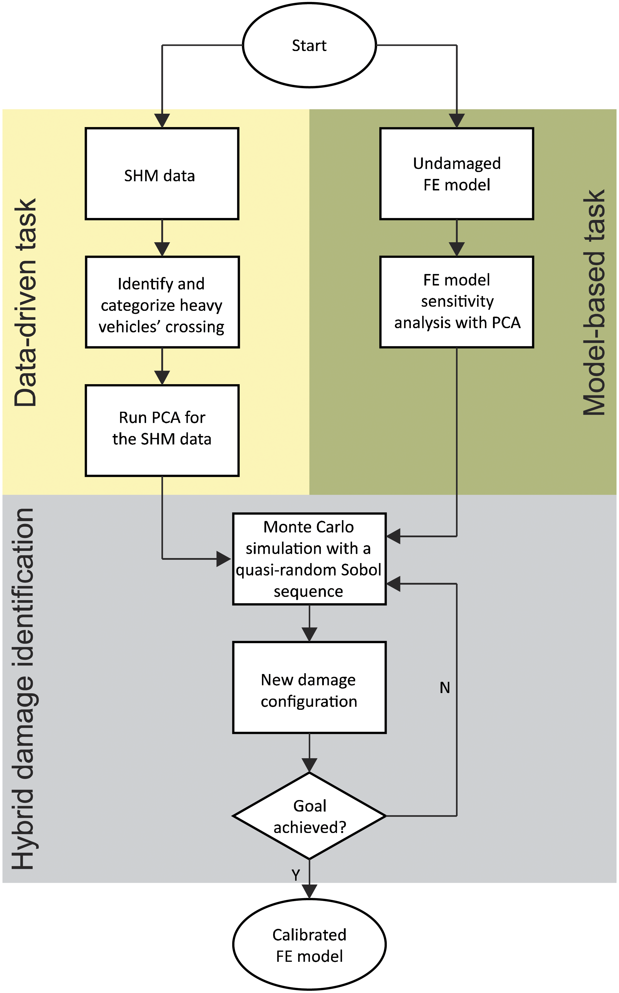

PCA of the SHM measurements

An important task to assure damage identification reliability is to characterize the load cases that will be assessed. For a bridge structure, it is reasonable to consider crossing a single heavy vehicle to the most representative external load. However, vehicles with different velocities, weights, lengths, and axle numbers cross the bridge at a random pace. Moreover, multiple heavy vehicles may cross the bridge simultaneously and in opposite directions. Therefore, a clustering algorithm was developed to identify when a single vehicle crosses the bridge and categorize the recorded vehicles’ crossing about their number of axles, total length, and travel direction. Representative load cases were then filtered and defined from the categorized traffic information having the following constraints:

• The crossing of a single heavy vehicle (in either direction);

• Number of identified axles equal or higher than two;

• Average velocity smaller than 30 m/s (108 km/h);

• Maximal strain at the bridge’s midpoint higher than 20 μm/m.

From the over 60 thousand recorded crossings, 11,470 were within those constraints and are summarized in Table 1.

Table 1.

Length categories by length interval and travel direction, with their respective number of vehicles’ crossings.

Group category	Length (L) interval in meters	Number of vehicles’ crossings		Group category	Length (L) interval in meters	Number of vehicles’ crossings
Group category	Length (L) interval in meters	Northern	Southern	Group category	Length (L) interval in meters	Northern	Southern
1	3 < L ≤ 4	698	32	7	9 < L ≤ 10	1476	597
2	4 < L ≤ 5	1583	56	8	10 < L ≤ 11	336	842
3	5 < L ≤ 6	756	150	9	11 < L ≤ 12	269	289
4	6 < L ≤ 7	202	154	10	12 < L ≤ 13	237	274
5	7 < L ≤ 8	691	302	11	13 < L ≤ 14	121	103
6	8 < L ≤ 9	1536	383	12	14 < L ≤ 15	49	71

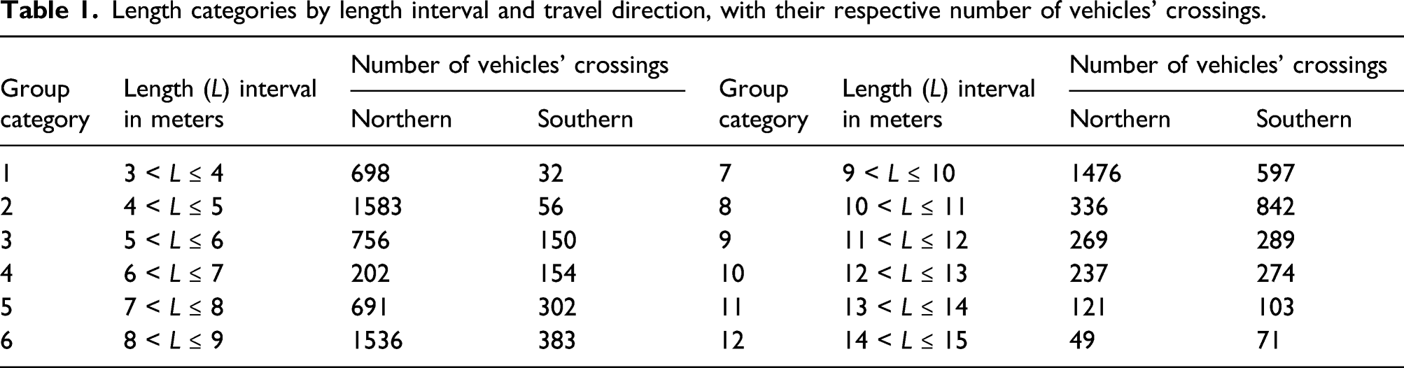
Figure 5(a) shows the raw strain signals for sensors S01 to S27 located underneath the northbound driving lane during a heavy vehicle’s crossing. All sensors’ signals are plotted in gray except for sensor S15, which is highlighted in blue. The sensors’ raw signals have a 20 Hz low-pass filter applied at the measuring unit. Figure 5(b) shows only the raw strain signal from sensor S15. To estimate the signal-to-noise ratio (SNR), the filtered signal for sensor S15, or in other words the estimated clean signal for sensor S15, is calculated by appling a Savitzky-Golay smoothing filter of polynomial order 3 and frame length 21 on sensor S15 raw signal, as depicted in Figure 5(b). A signal’s segment showing both raw and filtered signal are enlarged and displayed in the left top corner of Figure 5(b). The signal’s noise portinon is estimated by subtracting the filtered signal from the raw signal, as depcted on the right top corner in Figure 5(b). The SNR is then calculated using the MATLAB function snr(x,y), which returns the SNR in decibels of a signal, x, by computing the ration of its summed squared magnitude to that of the noise, y. The raw signal’s noise is small, with an amplitude smaller than ±1.0 μm/m, which leads to a SNR of 30 dB. A simplified SNR study was performed to assess the impact of the SNR in the PCA results by adding random white Gaussian SNR to the sensors’ signals. It was observed that SNR below +15 dB could cause changes in the PCA results that can be confused with changes due to structural degradation.

Figure 5.

Raw strain signals during the crossing of a heavy vehicle: (a) strain influence lines for sensors S01 to S27, with sensor S15 highlighted; (b) estimation of the signal-to-noise ratio for sensor S15.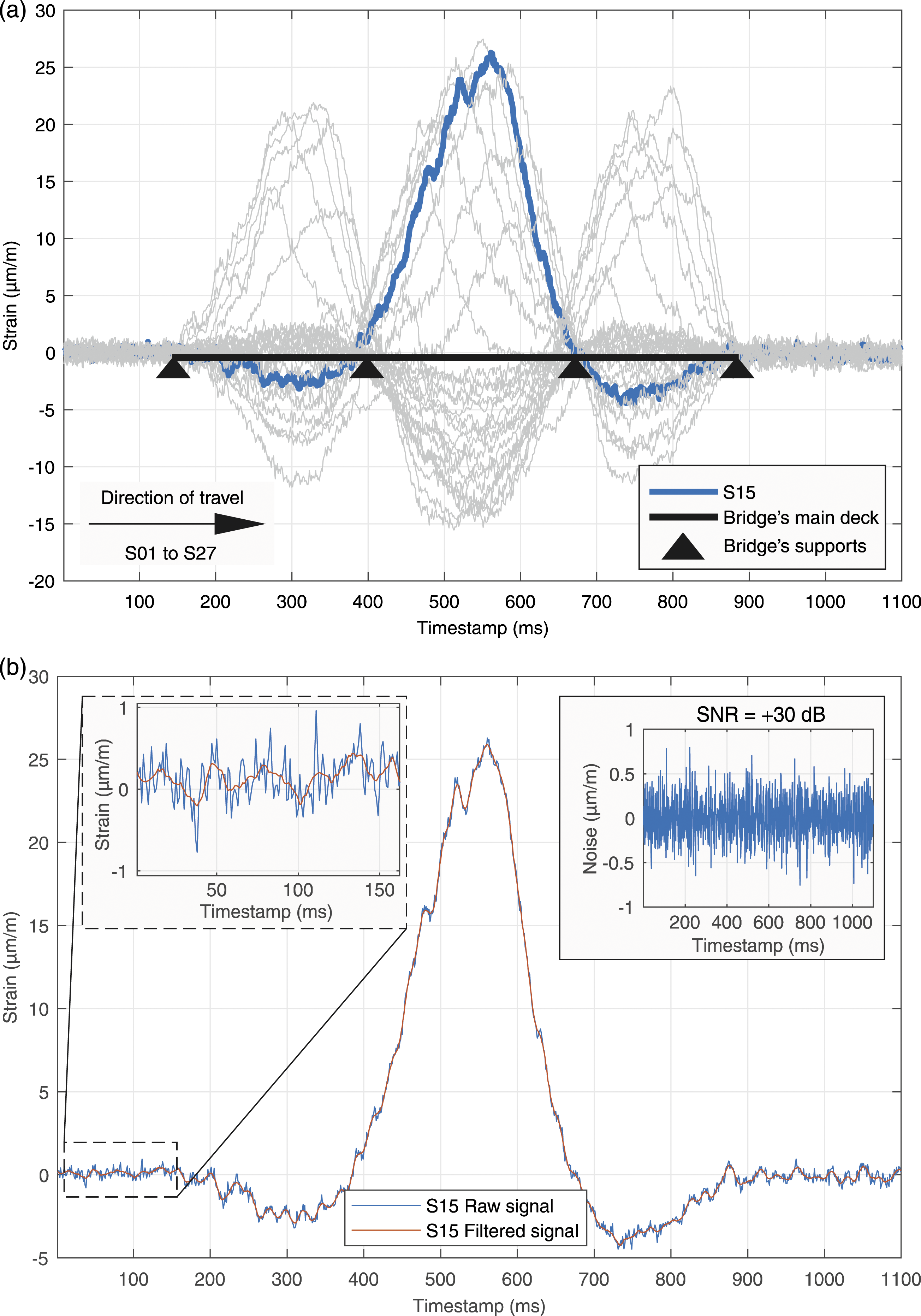

With the classified vehicle data, the PCA analysis is used to calculate each sensor’s contribution to the structural response. The vehicles’ crossings were first divided in the direction of travel (northern or southern) and then grouped about the vehicles’ length, as shown in Table 1. The vehicle lengths from 3 m to 15 m were divided by a one-m interval into 12 length categories. The categories were sorted by length because it is the parameter that impacts the most the strain histories’ response, considering vehicles within the road’s allowed weight.

Since sensors S01 to S27 are located underneath the northbound driving lane and sensors S28 to S54 underneath the southbound driving lane, the PCA was performed separately for sensors S01 to S27 considering only the northbound crossings, and for sensors S28 to S54 considering the southbound crossings. Therefore, for each PCA in either traveling direction, a total of 27 eigenvectors with 27 elements (one for each sensor) and 27 eigenvalues are generated. Only the analysis for the sensors in the northbound direction (sensors S01 to S27) will be depicted in this work.

Figure 6, for example, shows group 7 average PCA results for all its 1476 crossings in the northern direction. Only the first four eigenvectors with higher eigenvalues, that is, the first four principal components (PC), are analyzed as they explain over 95% of the system’s variance. Figure 6(a) depicts the first and second principal components’ eigenvectors, and Figure 6(b) the eigenvectors for the third and fourth principal components. In Figure 6(c), the individual first principal component’s eigenvector for sensors S07 and S14 are shown over time for a period of 1 year and 4 months. Their average values are depicted with dashed horizontal lines. Continuously horizontal lines define the range plus-minus two times their standard deviation for the period. The individual eigenvectors’ elements corresponding to each sensor are depicted with either circle or x-markers and connected with lines for visualization purposes. Figure 6(d) shows how much the first four principal components explain the system’s variance. From the first to the fourth PC, the variance explained were: 59.4%, 23.9%, 7.3%, and 4.6%.

Figure 6.

Average results of the PCA analysis for group 7 in northbound direction (S01 to S27). The lines connecting the eigenvectors’ elements are only to improve visualization and have no physical meaning: (a) eigenvectors for the first and second principal components (PC); (b) eigenvectors for the second and third PC; (c) eigenvectors’ elements for the first principal component over time—sensors S07 and S14; (d) variance explained by the first four PC.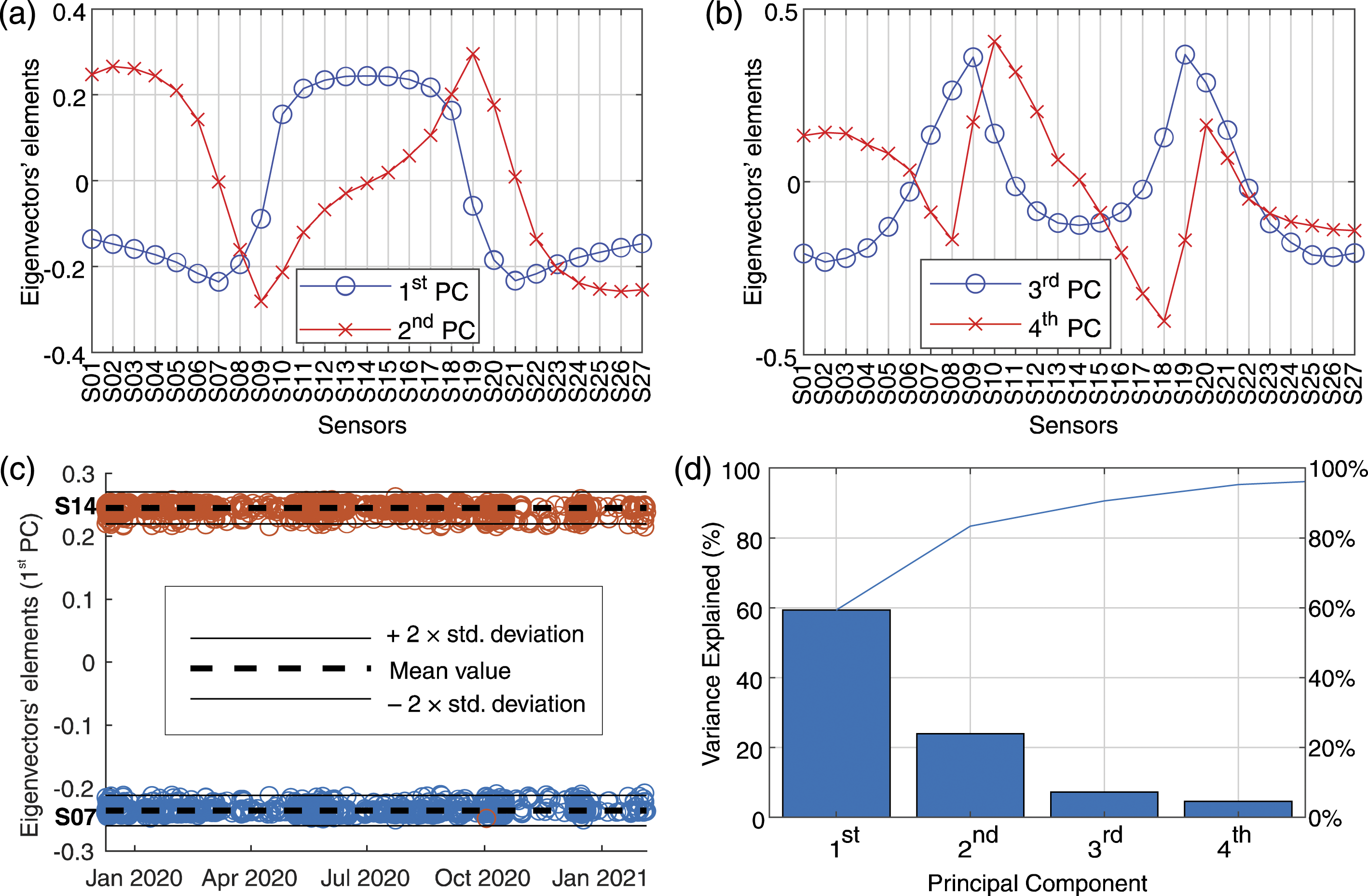

The same analysis shown in Figure 6 was performed for all length categories in Table 1 for both traveling directions. Similar graphics with the same behavior and shape in Figure 6(a) and Figure 6(b) were obtained. Figure 7 shows the PC elements’ changes from the PCA analysis of the length groups in Table 1 for the northbound crossings (sensors S01 to S27). The eigenvectors’ elements for each sensor and all length group categories were centered on having median zero and plotted as box plots for the first four pC. As expected, changes occur in the eigenvectors’ for different vehicle lengths. From the interquartile ranges (IQR), the influence of the vehicles’ length in the PC elements’ outcoming results can be assessed. In Figure 7(a), for example, the IQR from sensor S17 is eight times smaller than the IQR from sensor S10. Thus, sensor S10 is eight times more sensitive to changes than sensor S17 when the vehicle’s length varies.

Figure 7.

PCA changes of each sensor about the vehicle length groups for the SHM measurements. The PC elements were centered on having median zero and plotted as box plots: (a) first PC elements’ changes; (b) second PC elements’ changes; (c) third PC elements’ changes; (d) fourth PC elements’ changes.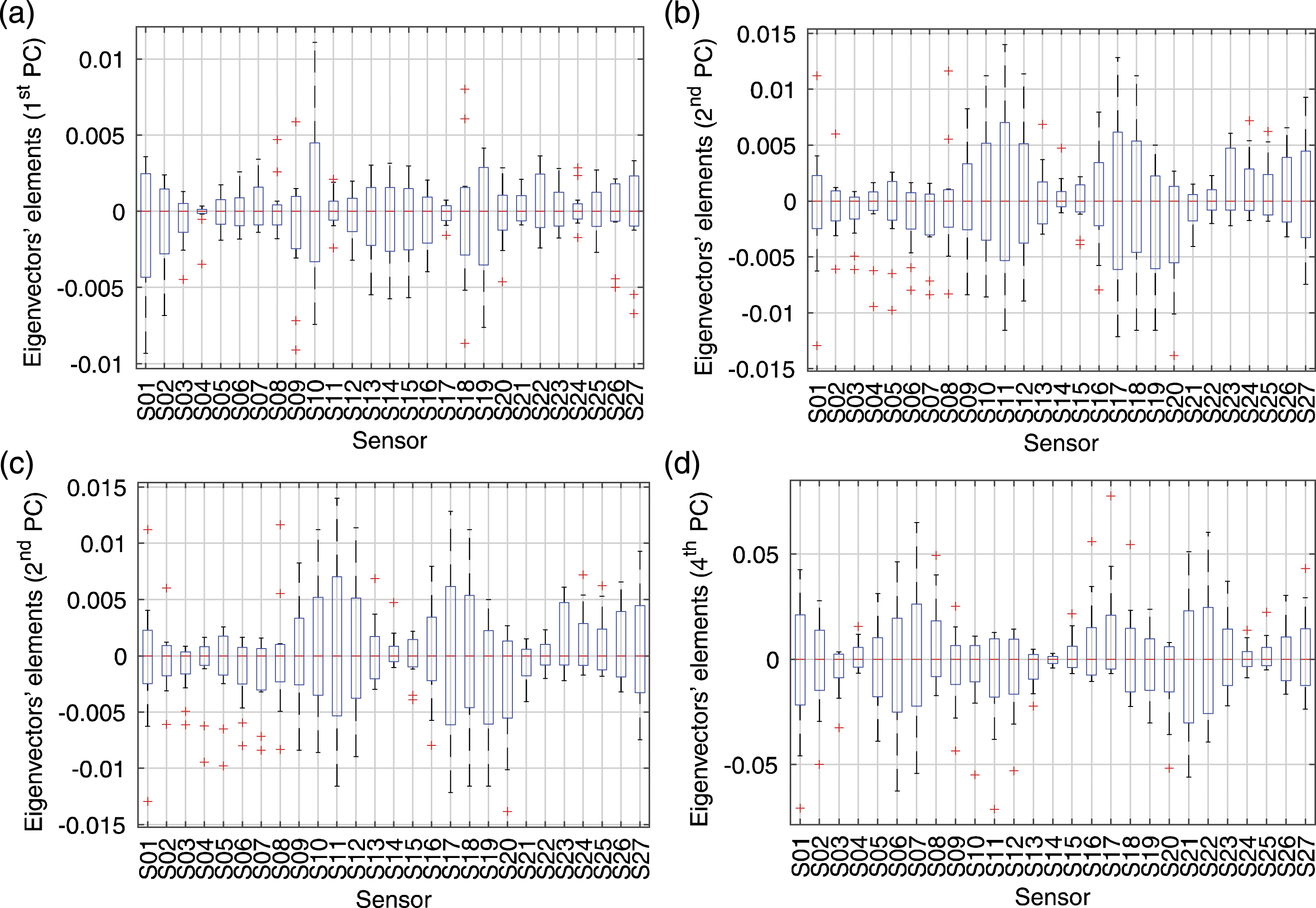

Therefore, for damage detection and model updating purposes, the PCA analysis should be applied for similar load cases to deliver reliable results. In traffic loads, for example, the measured data must be categorized into groups of vehicles by their length. For the long-term evaluation of the PC eigenvectors to detect structural changes, only pCs within the same vehicle length category should be analyzed together. Likewise, for model updating purposes, the FE model’s modeled load case should be compatible with a length category in the SHM measurements.

It is worth mentioning that the vehicles’ weight and average velocity within the same length category had little influence on the eigenvectors and eigenvalues during the PCA. Hence, the proposed workflow can be used without determining the actual load or stress levels and average velocity.

Finite element model sensitivity analysis

To use the PCA analysis in the model updating process, defining the PC eigenvectors’ elements sensitivity to structural changes in the FE model is necessary. Moreover, the FE model’s PCA results must be compatible and comparable to the PCA results from the SHM measurements. Therefore, the following workflow is proposed:

• Define a load train model compatible with a vehicle length category (Table 1) to simulate a vehicle’s crossing;

• Establish a “virtual” SHM in the FE model that mimics the results from the real SHM system;

• Apply the load train on the undamaged model and run the PCA analysis for the virtual SHM results;

• Introduce damage in various know cross-sections;

• For each damage case, apply the load train on the damaged model and run the PCA analysis for the virtual SHM results;

• Analyze the PC eigenvectors (from the first four PC) changes between the damage cases and the undamaged structure.

The chosen load train was the FLM4 according to the European norm Eurocode EN 1991–2.⁷¹ It has a total length of 11 m and a total weight of 490 kN. Figure 8 shows its dimensions and axle loads. The virtual SHM system was set up by organizing the beam elements in the FE model within each real LGFBG sensor’s gauge length. Figure 9(a) shows the arrangement of sensors S01 to S27 (northern travel direction) with the respective beam elements number in the FE model. For each beam element, the internal forces and deformations at a specific location are extracted by “stress points” in the cross-section definition. Figure 9(b) shows the two stress points that correspond to the two longitudinal LGFBG sensor line locations. Stress point BOTL (bottom left) provides the results for sensors S28-S54 and BOTR (bottom right) for sensors S01-S27.

Figure 8.

FLM4 load train used during the FE model sensitivity analysis. The dimensions are in meter.

Figure 9.

The virtual SHM system in the FE model: (a) beam elements’ number corresponding to each real sensor; (b) cross-section view with the stress points BOTL and BOTR at the longitudinal LGFBG sensor lines.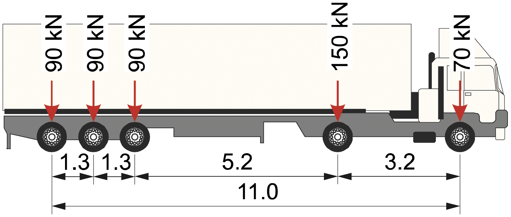

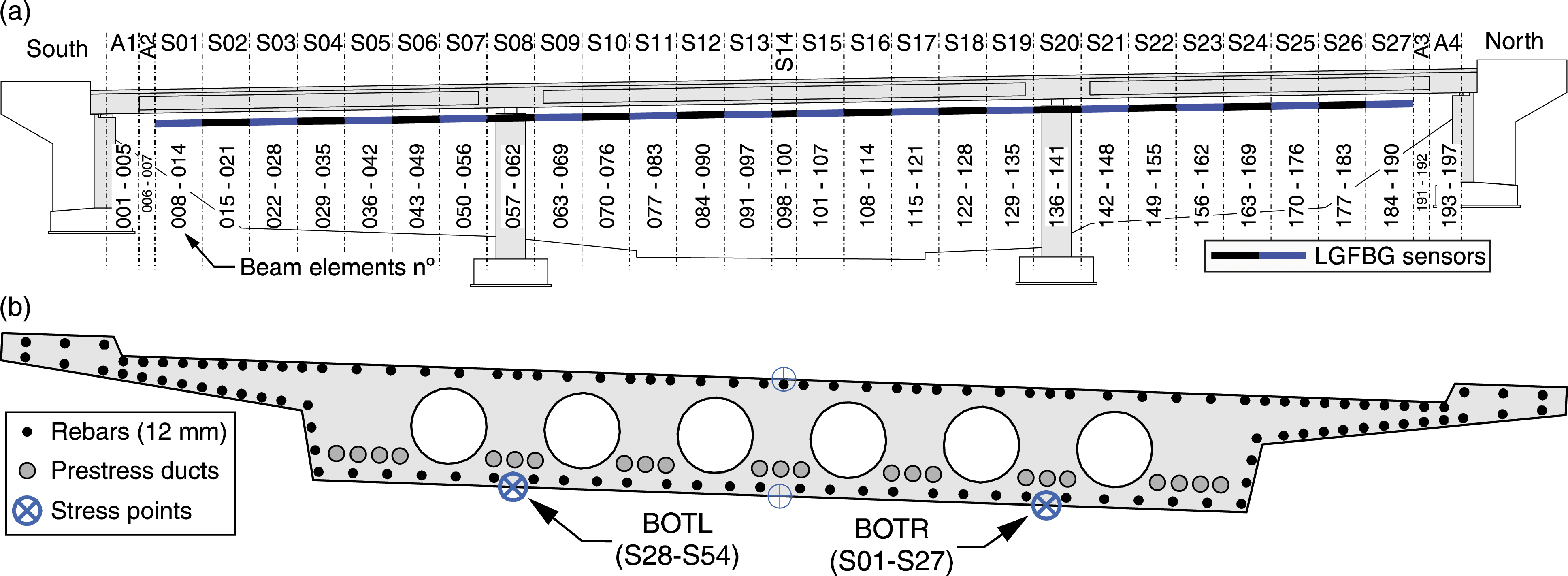
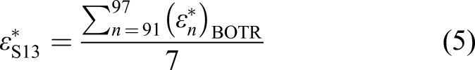
Since the real sensors measure the average deformation in their gauge length, the virtual sensors’ results are calculated by taking the average strain at their beam elements’ stress points, as follows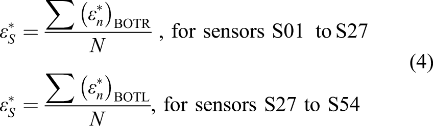

\begin{array}{l} ε_{S}^{*} = \frac{\sum^{} {(ε_{n}^{*})}_{BOTR}}{N}, for sensors S 01 to S 27 \\ ε_{S}^{*} = \frac{\sum^{} {(ε_{n}^{*})}_{BOTL}}{N}, for sensors S 27 to S 54 \end{array}

(4)where

ε_{S}^{*}

is the strain at virtual sensors S01 to S54,

ε_{n}^{*}

is the strain at the stress point of beam element n and N is the total number of beam elements, as shown in Figure 9(a). The measured strain at virtual sensor S13 for example, is given by

ε_{S 13}^{*} = \frac{\sum_{n = 91}^{97} {(ε_{n}^{*})}_{BOTR}}{7}

(5)With the virtual sensors results for the load train’s crossing, the PCA analysis results from the virtual SHM are compatible and comparable to the PCA results from the real SHM system.

Next, the damage cases are defined in the FE model by reducing selected beam elements’ bending stiffness. Twenty-seven mutually exclusive damages cases, one for each sensor in the longitudinal direction, were described and shown in Table 2.

Table 2.

Damage case definition and their stiffness reduction intensities.

Damage case	Description
DC01 to DC27 (DC28 to DC54)	Uniform 10% stiffness reduction in beam elements of sensor Sxx (corresponding to DCxx)

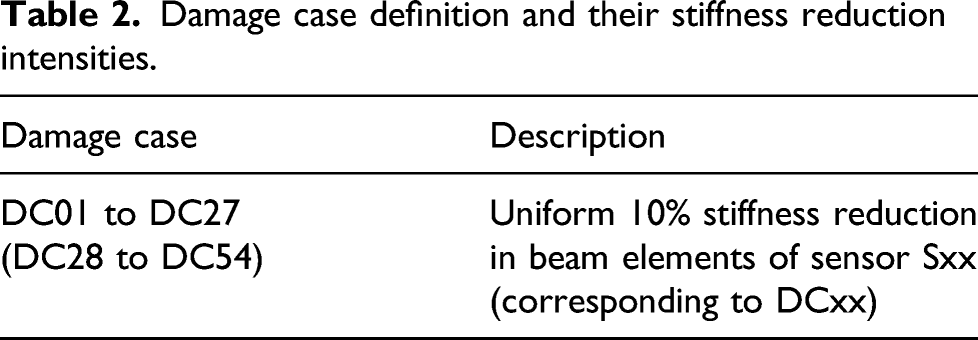
For each damage case, the load train was applied, and the PCA analysis of the virtual sensors’ results was calculated. Therefore, it is possible to assess how the principal components’ eigenvectors and their elements change for each damage case and which damage cases have more impact on the overall structural response. Since the results for the northbound (sensors S01 to S27) and southbound (sensors S28 to S54) are similar, only the northbound traffic is presented.

Figure 10 shows the virtual PC eigenvectors elements’ changes for damage cases D01 to D27 for sensors S01 to S27. Each of the four PC eigenvectors is analyzed separately in Figures 10(a) to (d). First, the virtual PC eigenvectors’ elements calculated for each damage case are depicted as box plots, with their values normalized to have a median zero. For example, in Figure 10(a) the first PC eigenvectors’ elements for sensors located in the regions S08-S10 and S18-S20 near the columns are more scattered when compared with the sensors in the spam segments, with much higher IQR and full range, meaning that those sensors are much more sensitive to structural changes. Next, the damage cases’ weight, that is, each damage case’s impact on the virtual PC eigenvectors’ changes, is plotted below the box plot as bars. The weights are calculated by computing the NRMSE between each damage cases and the undamaged case, and then normalized to having a range from 0 to 1, with 0 meaning no impact and 1 maximal impact. It can be observed that the eigenvector’s elements with higher change are also the damage locations that have the most impact on the overall structural response when damage is introduced there. The same observations are valid for the second, third, and fourth PC eigenvectors depicted in Figures 10(b) to (d). It is worth mentioning that a damaged location with a high impact on one PC eigenvector does not necessarily have the same influence on the other pCs eigenvectors. For the first PC eigenvector in Figures 10(a), (e), (g) damage at sensor S19 location has the most overall impact with a weight of 1.0, while in the second PC eigenvector, it has a minor effect with a weight of 0.19.

Figure 10.

Structural response sensitivity regarding the damage cases: (a) first PC sensitivity; (b) second PC sensitivity; (c) third PC sensitivity; (d) fourth PC sensitivity.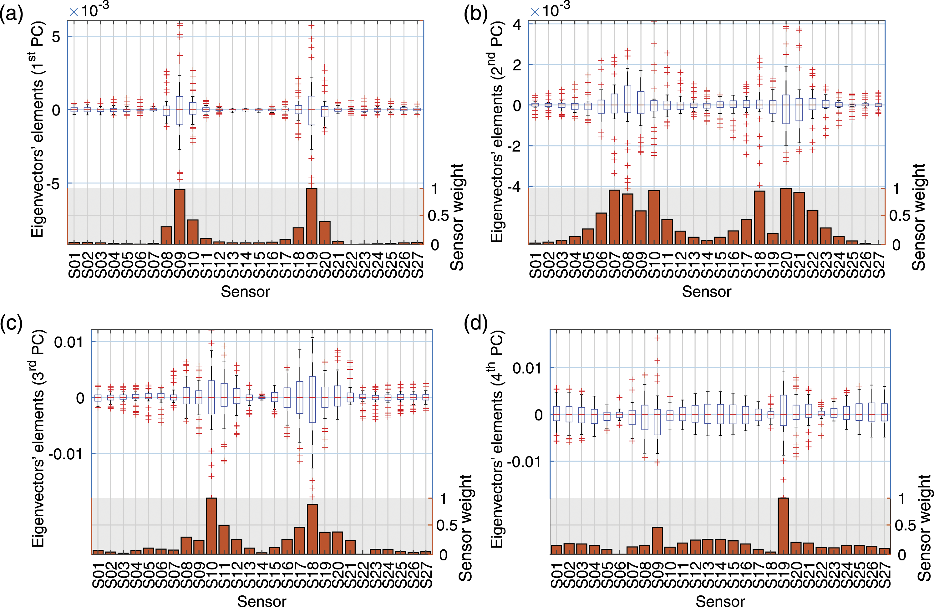

Figure 11 shows another unique approach to assess the structure’s sensitivity to damage. For each damage case D01 to D27, the relative difference $δ_{i, j}^{*}$ between the individual eigenvectors’ elements ${\hat{v}}_{i, j}^{*}$ and the eigenvector’s elements from the undamaged reference case $\bar{v_{i}}$ were calculated as follows

{(δ_{i, j}^{*} = \frac{{\hat{v}}_{i, j}^{*} - \bar{v_{i}}}{\bar{v_{i}}})}_{P C_{k}}, with {\begin{matrix} k = 1 to 4, corresponds to the first four P C \\ i = 1 to 27, is the PC elements of sensor i \\ j = 1 to 27, is the analyzed damage case j \end{matrix}

(6)With the relative difference matrix

δ_{i, j}^{*}

for each principal component k each individual change in the eigenvectors’ elements is known due to each damage case. Figure 11(a) depicts the relative difference matrix

δ_{i, j}^{*}

for the first principal component (k = 1) in a heatmap, where the lines correspond to the eigenvector’s element of sensor i for each damage case in column j .The relative differences and the color scale are normalized along each row to range from −1 to 1, allowing the visual assessment of the sensor’s sensitivities about the damage cases. Applying damage at a sensor location will not necessarily cause the most considerable perturbation at that sensor’s eigenvector element. Take sensor S19, for example. The foremost positive variations in sensor S19’s first PC eigenvector element happens when damage is introduced at sensors S15 to S17 (damage cases D15 to D17). Likewise, the most significant negative variations occur when damage is located on sensors S21 to S23 (damage cases D21 to D23).

Figure 11.

Heatmap with the individual PC elements’ changes for each mutually exclusive damage case location. Each line corresponds to a sensor PC element and is normalized to have a range from −1 to 1: (a) first PC elements; (b) second PC elements; (c) third PC elements; (d) fourth PC elements.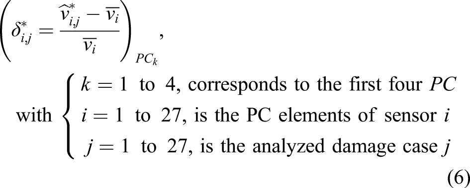

Moreover, a damage case can cause structural response changes at multiple sensor locations. Damage introduced at sensor S20 (damage case D20), for example, causes the highest negative variation in sensors S22 to S27 and the maximum positive changes in sensors S14 to S18 for the first PC eigenvector. Similar observations can be made for the second, third, and fourth PC eigenvectors’ elements in Figure 11(b) to Figure 11(d). Moreover, a sensor’s PC eigenvector element may experience changes with opposite signals considering different principal components. For example, if the damage is introduced at sensor S13 (damage case D13), sensor S16’s first PC eigenvector element is strongly reduced, while its second PC eigenvector element increases.

Finite element model updating

The proposed model updating process is based on the range-normalized root mean square error (NRMSE) optimization between the PCA results from the real and the virtual SHM systems. As mentioned before, the results for the northbound (sensors S01 to S27) and southbound (sensors S28 to S54) are alike. Therefore, only the results for the northbound traffic (sensors S01 to S27) are presented for the sake of representation.

First, the PCA results from group category 7 with northern travel direction (Table 1) are selected as the real reference case and the trainload LM4 type 3 as the reference load case for the virtual results. The process starts with the NRMSE for the undamaged FE model, which will be referenced from now on as the undamaged model. Next, a Monte Carlo objective function optimizes the NRMSE selecting an initial damaged model. Finally, the initial damaged model undergoes refinements in an iterative optimization procedure until the NRMSE result converges. The stages in the proposed model updating are described in this section.

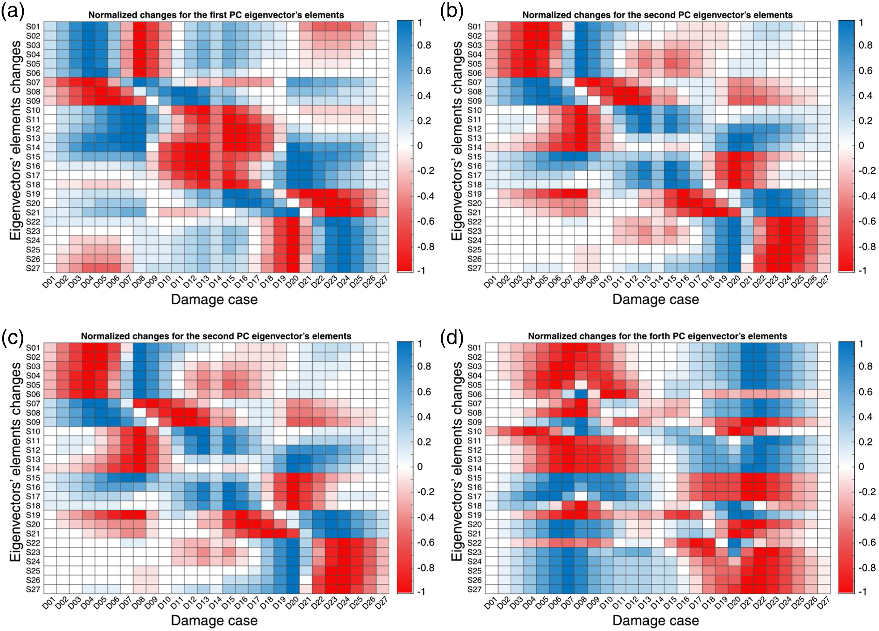
Figure 12 shows the results for the first four PC eigenvectors from the undamaged model and the real reference case (from Figure 6). The real reference PC eigenvectors’ elements are depicted with red circle markers and full lines, and the virtual PC eigenvectors’ elements with blue x-markers and dashed lines. The lines connecting the eigenvectors’ elements are only to improve visualization and have no physical meaning. The NRMSE for each PC is plotted in percentage, ranging from 1.96% for the first PC to 7.30% for the third component, with an overall average of 4.30%.

Figure 12.

Undamaged model PC eigenvectors results. The PC eigenvectors’ elements from the FE damaged model are represented with blue x-markers and dashed lines. The PC eigenvectors’ elements from the real reference SHM case are plotted with red circles and full lines. The lines connecting the eigenvectors’ elements are only to improve visualization and have no physical meaning. For each PC, the NRMSE is printed in percentage: (a) the first PC elements; (b) the second PC elements; (c) the third PC elements; (d) the fourth PC elements.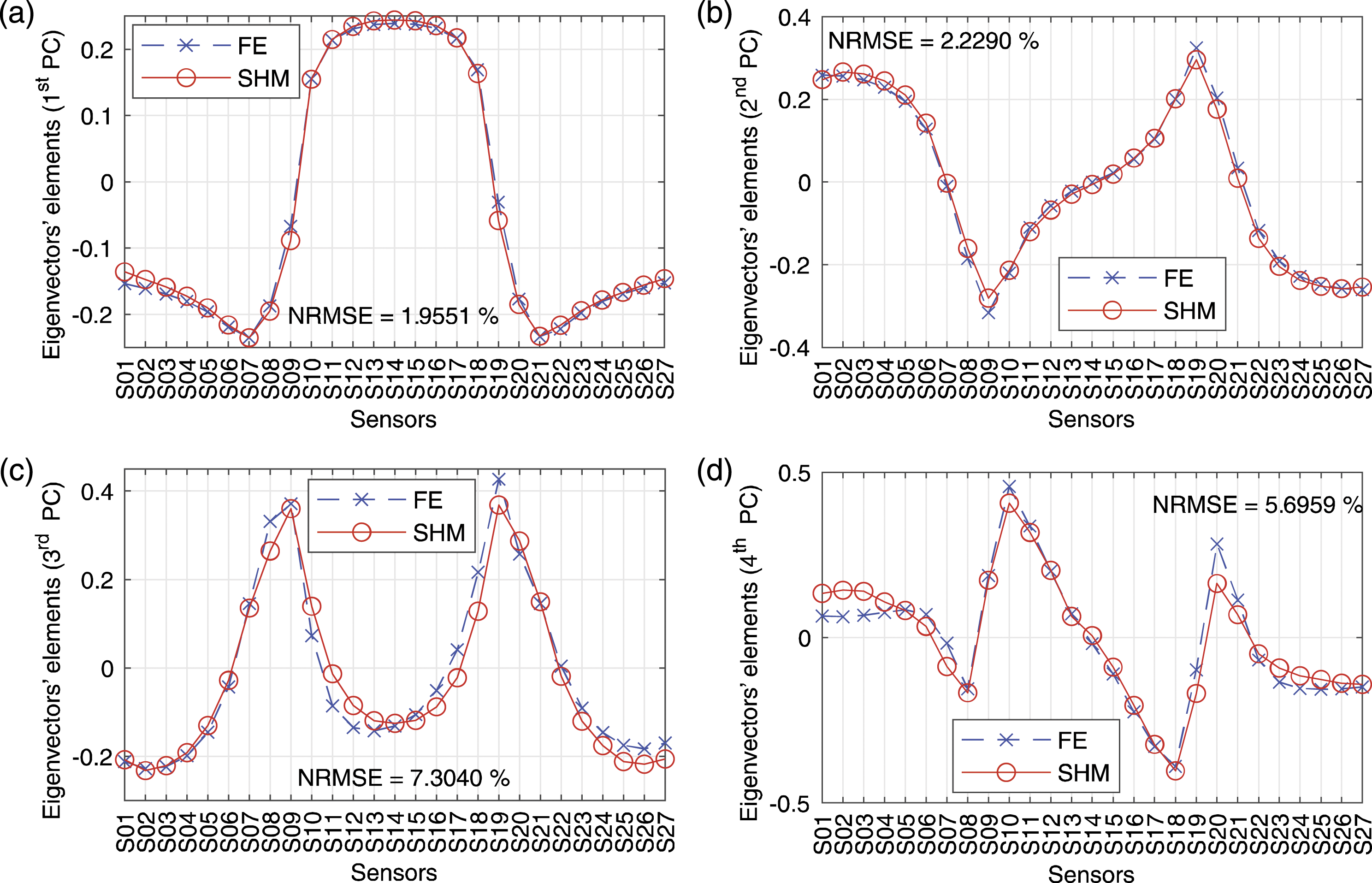

With the knowledge of how the virtual PC eigenvectors’ elements change for each mutually exclusive damage case in the virtual SHM, as shown in the Finite Element Model Sensitivity Analysis section (6), the combination of damage cases and damage intensities that most resembles the real structure behavior is searched with the objective function (7) to minimize the average NRMSE between the virtual PC eigenvectors’ elements and the real SHM PC eigenvectors’ elements results (8). However, it is unfeasible to run the FE analysis at the necessary amount of damage and intensity combinations to accurately target the objective function (7). Therefore, a Monte Carlo experiment is used to optimize a quasi-random sequence sampling of damage coefficients $ξ$ as shown in Figure 13.

The sequence ${[ξ]}_{j \times m}$ is a Sobol quasi-random sampling matrix with its elements ranging from 0 to 1. Each column $m$ is a sample vector with $j$ elements, where $j$ is the number of damage cases (Table 2). A zero element, $ξ_{j}^{m} = 0$ annulates the damage case $j$ , whereas an element with a value greater than zero, $ξ_{j}^{m} > 0$ means that the damage case $j$ acts proportionally with its value. In this work, a Sobol quasi-random sequence of 8 million sample vectors was used.

Figure 13.

Monte Carlo experiment to optimize the damage combination and intensities in the FE model.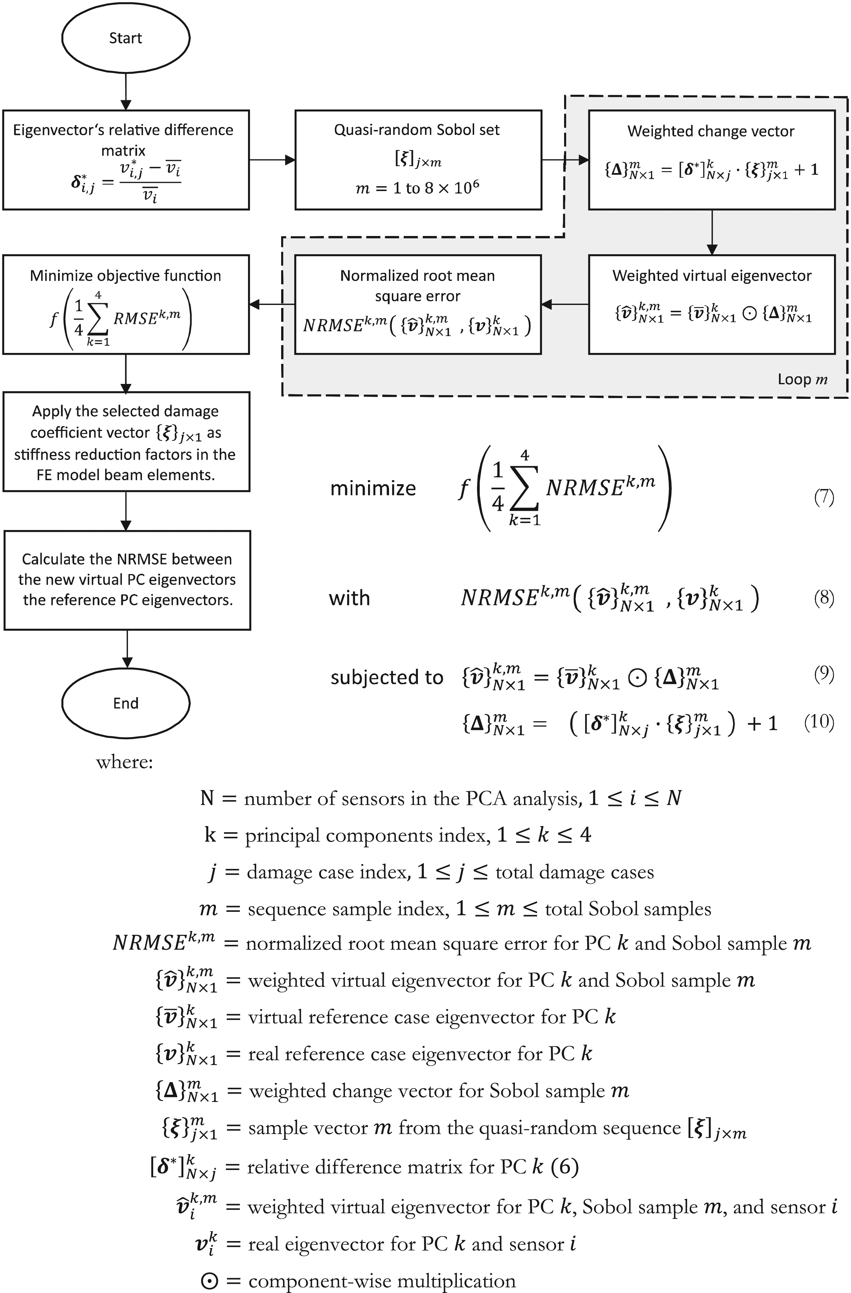

When the relative difference matrix ${[δ^{*}]}_{N \times j}^{k}$ (6) multiplies a sample vector ${ξ}_{j \times 1}^{m}$ from the Sobol sequence (10), the PC elements changes in sensor $i$ due to damage case $j$ are multiplied by the random number $ξ_{j}^{m}$ and added up, resulting in the weighted difference for each sensor $i$ Adding 1 to the weighted differences gives the weighted change vector ${Δ}_{N \times 1}^{m}$ which multiplied component-wisely by the reference virtual PC eigenvector elements ${\bar{v}}_{N \times 1}^{k}$ results in the weighted virtual PC eigenvector ${\hat{v}}_{N \times 1}^{k, m}$ (9). Next, the NRMSE between the weighted virtual PCs ${\hat{v}}_{N \times 1}^{k, m}$ and the real PC elements ${v}_{N \times 1}^{k}$ for the first to fourth PCs’ eigenvectors are calculated (8). Finally, the objective function (7) selects the Sobol sample vector ${ξ}_{j \times 1}^{m}$ with the damage coefficients resulting in the smaller average of the NRMSE.

Once the damage coefficient vector ${ξ}_{j \times 1}$ is selected, its elements are applied in the FE model beam elements as stiffness reduction factors ( $F A C S$ ) via customized scripts, which allows customizations in the FE model properties and functionalities, as follows

F A C S = 1 - 0.1 \times {ξ}_{j \times 1}

(11)

For example, if $ξ_{13} = 1$ $F A C S = 0.9$ and the beam elements within sensors S13 gauge-length will have a stiffness reduction equal to the full intensity of damage case D13, which is 10% stiffness reduction (Table 2). Now, if $ξ_{13} = 0.5$ damage case D13 is applied with half its intensity, resulting in a 5% stiffness reduction for the beam elements at sensor S13. Lastly, if $ξ_{13} = 0$ damage case D13 is annulated, and beam elements at sensor S13 suffer no stiffness reduction. The PCA analysis is performed for the damaged FE model’s traffic load results with the damaged factors applied to the beam elements. The NRMSE between the real reference PC eigenvector elements and the new virtual PC eigenvector elements is calculated. This first damage configuration will be from now on referred to as the initial damaged model.

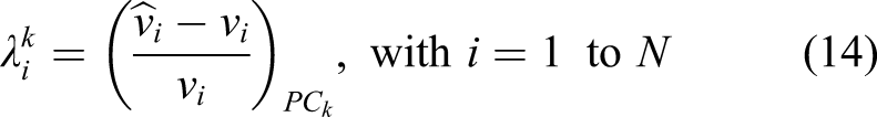
Finally, the initial damaged model undergoes refinements by applying correction from −20% to +20% on the initial damaged model’s stiffness reduction factors until the calculated eigenvectors’ NRMSE between iterations converges. This stage repeats the Monte Carlo workflow in Figure 13, but replacing and with (12) and (13), respectively, and ${[ξ]}_{j \times m}$ with the Sobol quasi-random sampling matrix ${[ψ]}_{j \times m}$ that has 8 million samples of damage correction vectors with elements ranging from −0.2 to 0.2, as follows

{\hat{v}}_{N \times 1}^{k, m} = {v}_{N \times 1}^{k} ○ . {Δ}_{N \times 1}^{m}

(12)

{Δ}_{N \times 1}^{m} = {λ}_{N \times 1}^{k} ○ . ({ψ}_{N \times 1}^{m} + 1)

(13)

λ_{i}^{k} = {(\frac{{\hat{v}}_{i} - v_{i}}{v_{i}})}_{P C_{k}}, with i = 1 to N

(14)

F A C S^{n e w} = F A C S ○ . ({ψ}_{N \times 1} + 1)

(15)where

{λ}_{N \times 1}^{k}

is the relative change vector between the PC elements from the last virtual damaged model and the real reference case, and

{ψ}_{N \times 1}^{m}

is the damage correction vector. The other variables have the exact definition as those given in Figure 13. Once the relative change vector

{ψ}_{N \times 1}

that results in the smallest NRMSE is selected, the new stiffness reduction factors are applied in the FE model. If

ψ_{13} = - 0.2

for example, the new stiffness reduction factor

F A C S_{13}^{n e w}

is equal to

0.8 \cdot F A C S_{13}

The described refinement process is repeated until the eigenvectors’ average NRMSE change between iterations converges. Figure 14 shows the entire model updating process, where the eigenvectors’ average NRMSE for each iteration is depicted with blue circles. The first iteration corresponds to the undamaged model and has an average NRMSE of 4.17%. After running the first iteration as described in Figure 13, the eigenvectors’ average NRMSE drops to 2.56%, which defines the initial damaged model. Next, the refinement process is repeated until the 18^th iteration, when the final damaged model with an average NRMSE of 2.48% is reached. The iterations’ average NRMSE gradient is plotted on the right y-axis and represented with a continuous orange line. The gradient oscillates until the 14^th iteration, starting to converge to zero up to the 18^th iteration.

Figure 14.

Average NRMSE during the model updating iterations. Iteration 1 represents the undamaged model, iteration 2 is the initial damaged model, and iteration 18 is the final damaged model. The convergence is shown as the NRMSE gradient.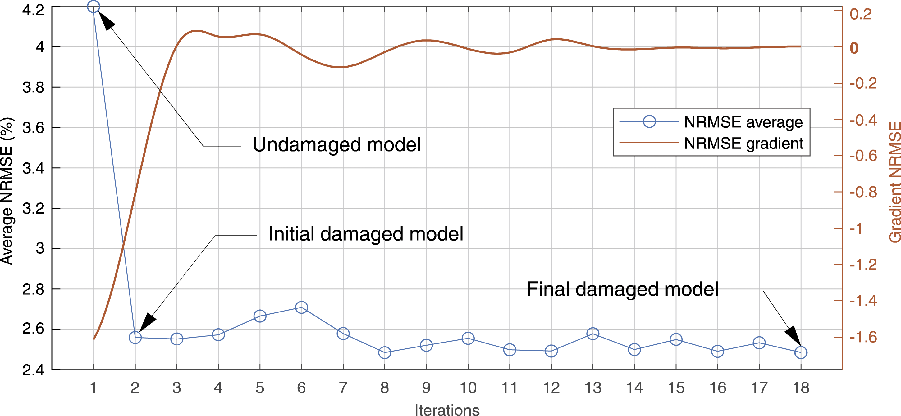

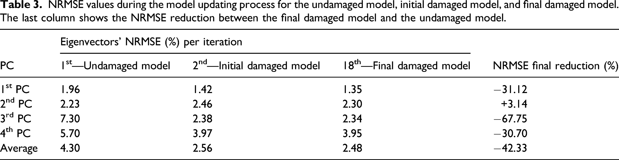
Table 3 shows the eigenvectors’ average NRMSE value for the undamaged model, the initial damaged model, and the final damaged model. The final NRMSE reduction between the final damaged and undamaged models is shown in the last column. The best improvement was in the third PC eigenvector, with an NRMSE decrease of 67.75%, followed by the first and fourth PC, showing reductions of 31.12% and 30.70%, and ending with the second PC, which was increased by 3.14%. The eigenvectors’ average NRMSE was reduced by 42.33%.

Table 3.

NRMSE values during the model updating process for the undamaged model, initial damaged model, and final damaged model. The last column shows the NRMSE reduction between the final damaged model and the undamaged model.

PC	Eigenvectors’ NRMSE (%) per iteration			NRMSE final reduction (%)
PC	1^st—Undamaged model	2^nd—Initial damaged model	18^th—Final damaged model	NRMSE final reduction (%)
1^st PC	1.96	1.42	1.35	−31.12
2^nd PC	2.23	2.46	2.30	+3.14
3^rd PC	7.30	2.38	2.34	−67.75
4^th PC	5.70	3.97	3.95	−30.70
Average	4.30	2.56	2.48	−42.33

Finally, Figure 15 shows the PC eigenvectors’ elements after the model updating process. The final damaged model’s eigenvector elements are depicted with blue x-markers and dashed lines, and PC eigenvectors’ elements for the real reference SHM case are shown with red circle markers and full lines. For each PC, the NRMSE is plotted in percentage. The overall NRMSE improvement can be visually observed by comparing the virtual PC results for the final damaged model in Figure 15, and the virtual PC results for the undamaged model in Figure 12.

Figure 15.

Principal components’ elements for the final damaged model. The PC elements from the FE damaged model are represented with blue x-markers and dashed lines. The PC elements from the real reference SHM case are plotted with red circles and full lines. For each PC, the NRMSE is printed in percentage: (a) first PC elements; (b) second PC elements; (c) third PC elements; (d) fourth PC elements.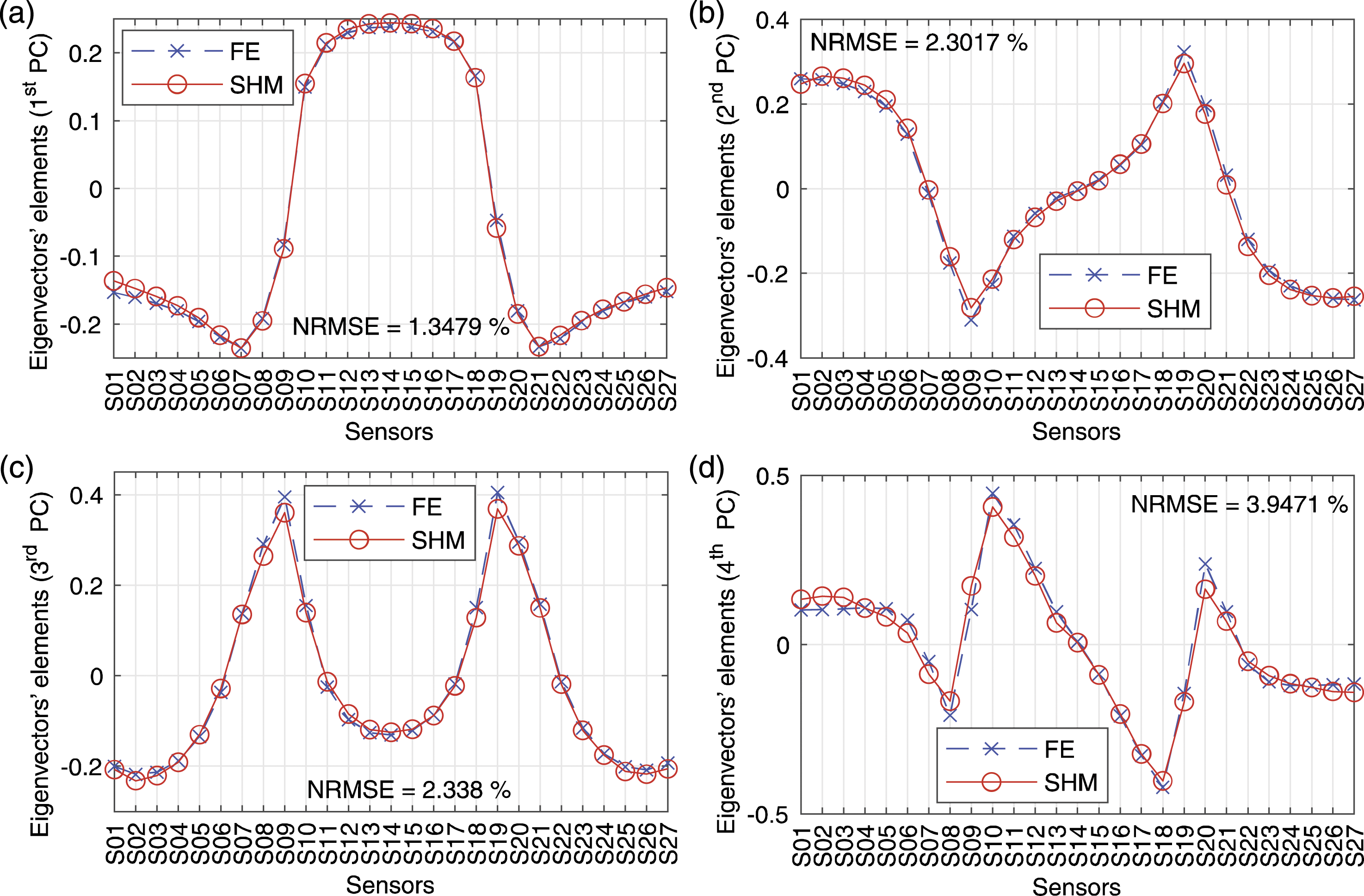

The stiffness reduction factors ( $F A C S$ ) in the final damaged FE model are depicted as a heatmap in Figure 16. The values correspond to the total stiffness reduction applied in the beam elements at each sensor location. A maximum stiffness reduction is observed at sensors S16 and sensors S09, with a decrease of 15.5% and 13.5%, respectively. The beam elements in the first spam (S01-S07) have a minor stiffness reduction, with reduction values inferior to 2%. Next, the last spam beam elements (S21-S27) have stiffness reduction values ranging from zero to 9.3%. Finally, the mid-spam has the most significant reduction factors, with values ranging from zero to 15.15%.

Figure 16.

Stiffness reduction factors ( $F A C S$ ) applied in the beam elements of the final damaged FE model.

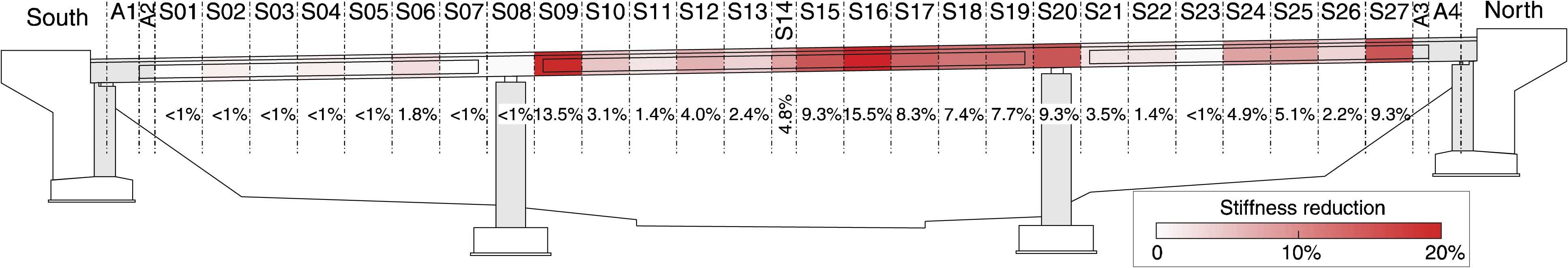
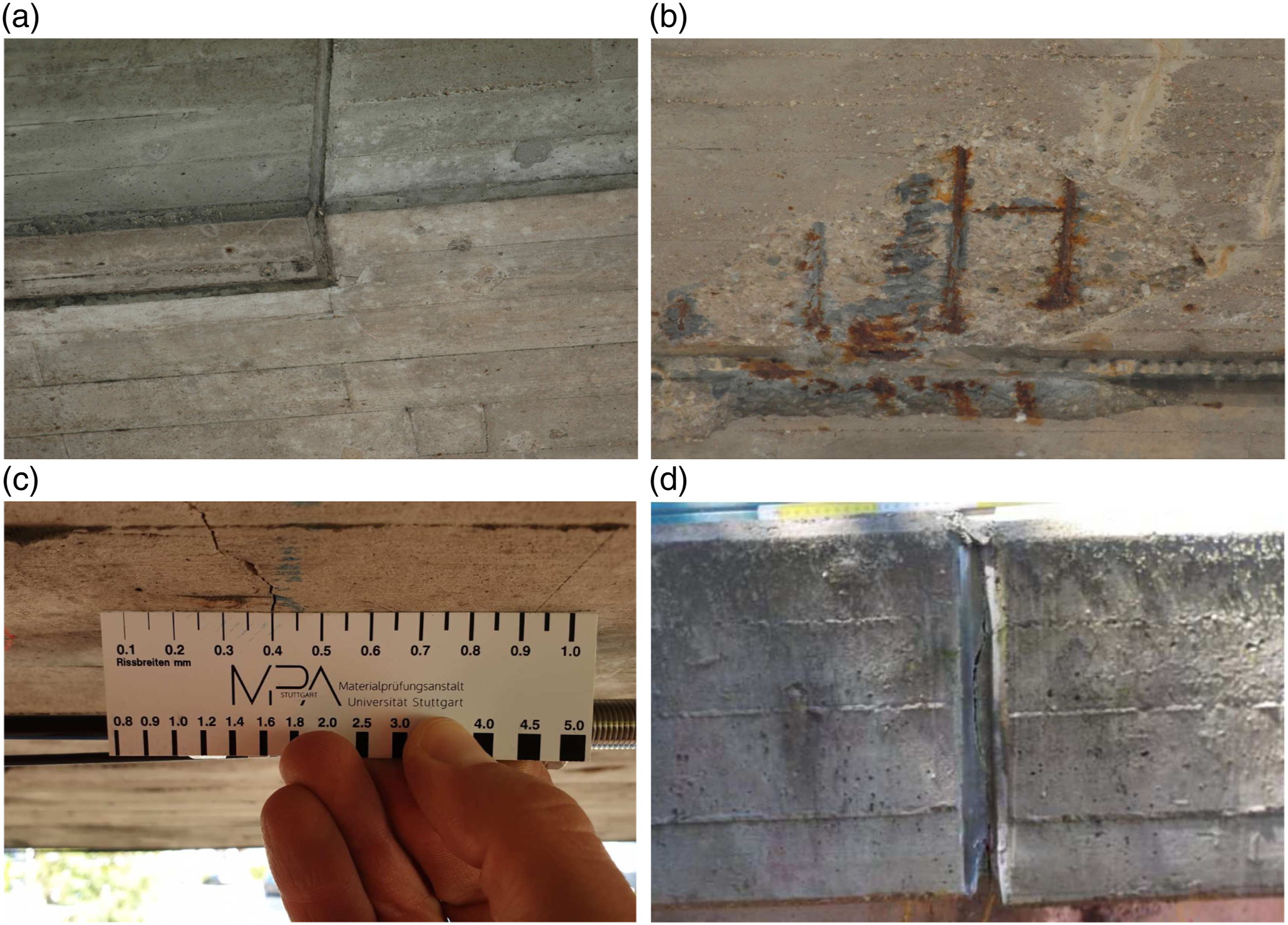
The facticity of the calibration results was verified by comparing the sections’ stiffness reductions with in-field visual data. The first spam comprised by sensors S01 to S06 is the bridge’s region with the least visual damage, which coincides with the small stiffness reduction factors. Figure 17 shows visible damages or structural discontinuities that could have caused the stiffness reduction in the regions of sections S09, S19, and S27. For example, in Figure 17(a), the constructional joint at sensor S09 is visible, where there is a change in the superstructure’s cross-section from hollow-core (spam) to massive (column’s region). Moreover, Figure 17(b) shows spalling concrete with exposed rebars at sensor S09. An excessive crack opening at sensor S19 is displayed in Figure 17(c) Finally, a constructional joint with visible cracking at sensor S27 is depicted in Figure 17(d).⁷²

Figure 17.

Visual damages and structural discontinuities: (a) constructional joint at sensor S09; (b) spalling concrete with exposed rebars at sensor S09; (c) excessive cracking at sensor S19; (d) constructional joint with cracking at sensors S27.⁷²

Nonetheless, the monitored bridge has a rupture-without-warning behavior⁷² typical of prestressed bridges of its age. It may take a large number of prestressed wire breaks until visible cracking takes place. That means that the ultimate resistance of a cross-section with wire breakage may be reached even before cracking is visible.⁷³ Therefore, stiffness reduction may happen due to prestressed wire breakage but without visible signs of damage, which may be the case, for example, for the stiffness reductions in the region of sensor S16.

The Monte Carlo approach allows the indirect evaluation of millions of damage combinations and intensities during the model updating process, which would be unfeasible if a FE simulation had to be executed for each damage scenario. For the model updating presented in Figure 14, a total of 144 million damage scenarios could be tested, while only 18 FE simulations were necessary.

Research constraints

The proposed methodology is a comprehensive demonstration for FE model updating and damage identification of a real-case SHM application. However, some limitations should be noted. First, the system operates for approximately 1 year, limiting the conclusions about the structure’s response to this short period. The second limitation concerns the sensor placement that prioritizes the longitudinal length coverage, leaving regions such as the deck slab’s sides and the columns unattended. Moreover, it was not possible yet to perform a load test at the monitored bridge to calibrate the SHM system. Although the measurement data quality is indisputable, allowing the indirect evaluation of the vehicle’s velocity, length, and number of axles, it is unfeasible to directly correlate the measured strains to the actual vehicles’ weight.

Additionally, the traffic load was simulated as static load steps in the FE model. Further investigations should improve the FE model to respond to dynamic loads to improve the structure’s response to vehicles’ crossings. Finally, damage introduction was considered only as stiffness reduction in the beam elements. Investigations are needed to evaluate the influence of other damage phenomes, such as unequal foundation settlement and changes in the supports’ boundary condition.

Conclusions

The authors presented a hybrid methodology that combines data-driven and FE model updating approaches to quantify the extent of local damage regarding stiffness reduction of an existing prestressed concrete bridge using a high LGFBG sensor-count SHM system. The principal component analysis (PCA) of the SHM data was used to access the structural response due to categorized traffic loadings. A virtual SHM system that mimics the behavior of the deployed SHM was implemented in the FE model, and simulations with a trainload compatible with the categorized vehicles’ crossings were performed. The PCA results from the virtual SHM were then used to optimize the model updating process. Next, the eigenvectors that explain up to 95% of the system static response’s variance were considered together. A Monte Carlo simulation was implemented to allow the indirect simulation of millions of damage combinations and intensities scenarios and minimize the NRMSE error between the virtual PCA results from the FE model and the real PCA results from the SHM system.

From the results presented in this work, the following conclusions are drawn:

• The use of long-gauge FBG sensors and their multiplexing capability enhances the sensor count for an optimum SHM area coverage. The adopted solution allows measuring the average strain within the two-m gauge length along the two quasi-distributed sensor arrays located underneath both driving lanes and covering their complete length. With intelligent data acquisition and data management, this configuration allows the implementation of feature extraction techniques, such as the PCA, to evaluate the structural response due to traffic-induced loading and access the sensors’ contribution to the driving principle governing the system’s behavior. The extracted features can be used as a target parameter to optimize the FE model updating process and detect anomalous structural behavior.

• In statically indeterminate structures, changes detected by data-driven analysis may result from multiple damages cases rather than damage located only at the sensor that presented abnormal behavior. Hence, changes in an individual sensor’s response should not be interpreted as damages limited to that sensor’s location. Moreover, a sensor’s response may change inversely proportional to damages in different locations. Therefore, a sensitivity analysis was implemented to estimate the impact of mutually exclusive damage cases in the FE model PCA results. It could be concluded that damage at a sensor’s location can impact the PCA results at multiple locations. Moreover, the PCA result of an individual sensor can be influenced by damage at other locations. In this sense, the model updating process should not treat each sensor’s response individually but take complete account of the sensors’ sensitivity to the structure changes.

• Given the stochastic nature of damage occurrences, it would be unfeasible to simulate the necessary FE models with different damage scenarios to optimize the model’s updating objective function accurately. Therefore, a Monte Carlo simulation was implemented. A quasi-random Sobol sequence with millions of combinations of damage location and intensity is indirectly used to optimize the model updating process. The Monte Carlo simulation is repeated for each FE simulation step, allowing the objective function optimization with only 18 FE simulation iterations.

• The PCA analysis of a quasi-distributed sensor array covering the structure’s complete length can confidently extract the driving principles of the structure’s static response during short and individual vehicles’ crossings and eliminate external influences such as environmental and operation variations. The damage identification reliability was improved by considering during the Monte Carlo simulation and optimization not only the eigenvector that represents the first principal component (PC) but all the eigenvectors that together explain up to 95% of the static response’s variance.

The reliable estimation of the extent of local damage leads to a rational structural conditional assessment. For example, the damaged FE model can be used to perform design checks to verify if the structure meets safety and serviceability requirements. Moreover, visual inspections and in situ non-destructive tests could be prioritized in the locations where damage is most likely to be present. Even more, the monitoring in combination with the FE model and proposed methodology provides continuous information on developing stiffness reduction and the acuteness of rehabilitation measures. Finally, the remaining structural lifetime can be locally assessed, allowing the optimization of interventions and repairs.

Footnotes

Acknowledgements

The authors are incredibly grateful to Ronald Blochwitz, Wolfgang Bonz, and the entire Unit 43 at the RPS for supporting this project; Andrej Tichý, Tomáš Šalát, and Peter Löwy from Sylex s. r.o, and José Monteiro and Daniel Ribeiro from HBM FiberSensing S.A. for their technical support and insights on FBG sensing technology; Rebekka Fackler for her assistance during the SHM system’s conception and deployment; and Helmut Ernst and Michael Schreiner from the MPA Stuttgart for their support during the experiment design and the SHM system’s deployment.

Funding

The author(s) disclosed receipt of the following financial support for the research, authorship, and/or publication of this article: This work was collectively funded by the research agency CAPES—Brazilian Federal Agency for Support and Evaluation of Graduate Education (grant no. 001), the Universidade Federal dos Vales do Jequitinhonha e Mucuri (UFVJM, Brazil), the Materials Testing Institute University of Stuttgart (MPA, Germany), and the Regierungspräsidium Stuttgart (RPS, Germany).

Data availability statement

The data presented in this study are available on request from the corresponding author.

ORCID iD

Felipe IH Sakiyama

References

Mechitov

Kim

, et al. Efficient time synchronization for structural health monitoring using wireless smart sensor networks. Struct Control Health Monit 2016; 23: 470–486.

Cho

Giles

Spencer

. System identification of a historic swing truss bridge using a wireless sensor network employing orientation correction. Struct Control Health Monit 2015; 22: 255–272.

Lynch

. An overview of wireless structural health monitoring for civil structures. Philosophical Trans R Soc A: Math Phys Eng Sci 2007; 365: 345–372.

Jang

Sim

, et al. Full-Scale Decentralized Damage Identification Using Wireless Smart Sensors. In: Tomizuka

(ed). San Diego, CA, USA. SPIE, 2010.

Spencer

Ruiz-Sandoval

Kurata

. Smart sensing technology: Opportunities and challenges. Struct Control Health Monit 2004; 11: 349–368.

Sakiyama

FIH

Lehmann

Garrecht

. Structural health monitoring of concrete structures using fibre-optic-based sensors: A review. Mag Concrete Res 2021; 73: 174–194.

Aeran

Acosta

Siriwardane

, et al. A nonlinear fatigue damage model: Comparison with experimental damage evolution of S355 (SAE 1020) structural steel and application to offshore jacket structures. Int J Fatigue 2020; 135: 105568.

Wang

Mao

Spencer

. A monitoring-based approach for evaluating dynamic responses of riding vehicle on long-span bridge under strong winds. Eng Structures 2019; 189: 35–47.

Meng

Zhu

Wang

. Numerical prediction of long-term deformation for prestressed concrete bridges under random heavy traffic loads. J Bridge Eng 2019; 24: 4019107.

10.

Sanio

Löschmann

Mark

, et al. Bauwerksmessungen versus rechenkonzepte zur beurteilung von spannstahlermüdung in betonbrücken. Bautechnik 2018; 95: 99–110.

11.

Adriaans

Ahrens

Eisler

, et al. Lebensdauerberechnung mit praxisüblicher software. Beton- und Stahlbetonbau 2016; 111: 278–287.

12.

Sohn

Farrar

Hemez

, et al. A Review of Structural Health Monitoring Literature: 1996–2001: Technical Report LA-13976-MS. NM, USA: Los Alamos National Laboratory, 2004.

13.

Abdel Wahab

De Roeck

. Damage detection in bridges using modal curvatures: Application to a real damage scenario. J Sound Vibration 1999; 226: 217–236.

14.

Saraf

. Evaluation of existing RC slab bridges. J Perform Construct Facil 1998; 12: 20–24.

15.

Aktan

Farhey

Helmicki

, et al. Structural identification for condition assessment: Experimental arts. J Struct Eng 1997; 123: 1674–1684.

16.

Aktan

Farhey

Brown

, et al. Condition assessment for bridge management. J Infrastructure Syst 1996; 2: 108–117.

17.

Brownjohn

Xia

Hao

, et al. Civil structure condition assessment by FE model updating:. Finite Elem Anal Des 2001; 37: 761–775.

18.

Meixedo

Santos

Ribeiro

, et al. Damage detection in railway bridges using traffic-induced dynamic responses. Eng Structures 2021; 238: 112189.

19.

Catbas

Kijewski-Correa

Aktan

. Structural Identification of Constructed Systems: Approaches, Methods, and Technologies for Effective Practice of St-Id. Reston Virginia: American Society of Civil Engineers, 2013.

20.

Baggio

Sabbatini

Santini

, et al. Comparison of different finite element model updates based on experimental onsite testing: The case study of San Giovanni in Macerata. J Civil Struct Health Monit 2021; 11(3): 767-790

21.

Sehgal

Kumar

. Structural dynamic model updating techniques: A state of the art review. Arch Comput Methods Eng 2016; 23: 515–533.

22.

Hong

Yang

, et al. Finite element model updating of flexural structures based on modal parameters extracted from dynamic distributed macro-strain responses. J Intell Mater Syst Structures 2015; 26: 201–218.

23.

Okasha

Frangopol

Orcesi

. Automated finite element updating using strain data for the lifetime reliability assessment of bridges. Reliability Eng Syst Saf 2012; 99: 139–150.

24.

Goulet

Kripakaran

Smith

IFC

. Multimodel structural performance monitoring. J Struct Eng 2010; 136: 1309–1318.

25.

Kumar

Biswas

Dhang

. Time series-based SHM using PCA with application to ASCE benchmark structure. J Civil Struct Health Monit 2020; 10: 899–911.

26.

Kromanis

Kripakaran

. Predicting thermal response of bridges using regression models derived from measurement histories. Comput Structures 2014; 136: 64–77.

27.

Cavadas

Smith

IFC

Figueiras

. Damage detection using data-driven methods applied to moving-load responses. Mech Syst Signal Process 2013; 39: 409–425.

28.

Sarmadi

Entezami

Salar

, et al. Bridge health monitoring in environmental variability by new clustering and threshold estimation methods. J Civil Struct Health Monit 2021; 11: 629-644

29.

Zhu

Jin

, et al. A temperature-driven MPCA method for structural anomaly detection. Eng Structures 2019; 190: 447–458.

30.

Entezami

Shariatmadar

. An unsupervised learning approach by novel damage indices in structural health monitoring for damage localization and quantification. Struct Health Monit 2018; 17: 325–345.

31.

Waibel

Schneider

Keller

, et al. A strain sensor based monitoring and damage detection system for a two-span beam bridge. In: Powers

Frangopol

Al-Mahaidi

, et al. (eds) Maintenance, Safety, Risk, Management and Life-Cycle Performance of Bridges: Proceedings of the Ninth International Conference on Bridge Maintenance, Safety and Management (IABMAS 2018), Melbourne, Australia, 9–13 July 2018, pp. 1627–1634. Milton: Chapman and Hall/CRC; 2018.

32.

Laory

Trinh

Posenato

, et al. Combined model-free data-interpretation methodologies for damage detection during continuous monitoring of structures. J Comput Civil Eng 2013; 27: 657–666.

33.

Laory

Trinh

Smith

IFC

. Evaluating two model-free data interpretation methods for measurements that are influenced by temperature. Adv Eng Inform 2011; 25: 495–506.

34.

Posenato

Kripakaran

Inaudi

, et al. Methodologies for model-free data interpretation of civil engineering structures. Comput Structures 2010; 88: 467–482.

35.

Posenato

Lanata

Inaudi

, et al. Model-free data interpretation for continuous monitoring of complex structures. Adv Eng Inform 2008; 22: 135–144.

36.

Malekzadeh

Atia

Catbas

. Performance-based structural health monitoring through an innovative hybrid data interpretation framework. J Civil Struct Health Monit 2015; 5: 287–305.

37.

Chen

. Multi-scale finite element model updating of highway bridge based on long-gauge strain response. In: Powers

Frangopol

Al-Mahaidi

38.

Cawley

. Structural health monitoring: Closing the gap between research and industrial deployment. Struct Health Monit 2018; 17: 1225–1244.

39.

Wong

, et al. Statistical analysis of stress spectra for fatigue life assessment of steel bridges with structural health monitoring data. Eng Structures 2012; 45: 166–176.

40.

Catbas

Gokce

Gul

. Nonparametric analysis of structural health monitoring data for identification and localization of changes: Concept, lab, and real-life studies. Struct Health Monit 2012; 11: 613–626.

41.

Liu

, et al.. Energy damage detection strategy based on strain responses for long-span bridge structures. J Bridge Eng 2011; 16: 644–652.

42.

Metzger

Huckelbridge

. Temporal Nature of Fatigue Damage in Highway Bridges. Quincy MA: National Fire Protection Assoc, 2009.

43.

Zhou

. Assessment of bridge remaining fatigue life through field strain measurement. J Bridge Eng 2006; 11: 737–744.

44.

Howell

Shenton

. System for in-service strain monitoring of ordinary bridges. J Bridge Eng 2006; 11: 673–680.

45.

Alampalli

Lund

. Estimating fatigue life of bridge components using measured strains. J Bridge Eng 2006; 11: 725–736.

46.

Chung

Kim

, et al. Deflection estimation of a full scale prestressed concrete girder using long-gauge fiber optic sensors. Construction Building Mater 2008; 22: 394–401.

47.

Glisic

. Influence of the gauge length on the accuracy of long-gauge sensors employed in monitoring of prismatic beams. Meas Sci Technol 2011; 22: 35206.

48.

You

Ren

Song

. A novel OFDR-based distributed optical fiber sensing tape: Design, optimization, calibration and application. Smart Mater Structures 2020; 29: 105017.

49.

Sieńko

Zych

Bednarski

, et al. Strain and crack analysis within concrete members using distributed fibre optic sensors. Struct Health Monit 2019; 18: 1510–1526.

50.

Barrias

Casas

Villalba

. Embedded distributed optical fiber sensors in reinforced concrete structures-a case study. Sensors (Basel, Switzerland) 2018; 18: 980

51.

Davis

Hoult

Bajaj

, et al. Distributed sensing for shrinkage and tension stiffening measurement. ACI Struct J 2017; 114: 753–764.

52.

Webb

Vardanega

Hoult

, et al. Analysis of fiber-optic strain-monitoring data from a prestressed concrete bridge. J Bridge Eng 2017; 22: 5017002.

53.

Butler

Elshafie

MZEB

, et al. Evaluating prestress losses in a prestressed concrete girder railway bridge using distributed and discrete fibre optic sensors. Construction Building Mater 2020; 247: 118518.

54.

Monsberger

Lienhart

. Distributed fiber optic shape sensing along shotcrete tunnel linings: Methodology, field applications, and monitoring results. J Civil Struct Health Monit 2021; 11: 337–350.

55.

Siwowski

Rajchel

Howiacki

, et al. Distributed fibre optic sensors in FRP composite bridge monitoring: Validation through proof load tests. Eng Structures 2021; 246: 113057.

56.

Ouyang

Chen

Huangfu

, et al. Application of distributed temperature sensing for cracking control of mass concrete. Construction Building Mater 2019; 197: 778–791.

57.

Bado

Casas

. A review of recent distributed optical fiber sensors applications for civil engineering structural health monitoring. Sensors (Basel, Switzerland) 2021; 21: 1818

58.

Prohaska

Snitzer

Chen

, et al. Fiber optic Bragg grating strain sensor in large-scale concrete structures. In: Claus

Rogowski

(eds) Fiber Optic Smart Structures and Skins V. Boston, MA: SPIE; 2015, pp. 286–294.

59.

Yang

, et al. Damage identification and bearing capacity evaluation of bridges based on distributed long-gauge strain envelope line under moving vehicle loads. J Intell Mater Syst Structures 2016; 27: 2344–2358.

60.

Zhang

Xia

Cheng

, et al. Strain flexibility identification of bridges from long-gauge strain measurements. Mech Syst Signal Process 2015; 62-63: 272–283.

61.

Zhang

. Simultaneously identifying displacement and strain flexibility using long-gauge fiber optic sensors. Mech Syst Signal Process 2019; 114: 54–67.

62.

Yang

, et al. Damage identification method for continuous girder bridges based on spatially-distributed long-gauge strain sensing under moving loads. Mech Syst Signal Process 2018; 104: 415–435.

63.

Huang

. Monitoring and structural analysis of a rehabilitated box girder bridge based on long-gauge strain sensors. Struct Health Monit 2018; 17: 586–597.

64.

Sakiyama

FIH

Lehmann

Garrecht

. A novel runtime algorithm for the real-time analysis and detection of unexpected changes in a real-size shm network with quasi-distributed fbg sensors. Sensors 2021; 21: 2871.

65.

Wüstholz

. Instandsetzung oder Neubau von Massivbrücken?: Erfahrungen und davon abgeleitete Ansätze. In: Bundesanstalt für Wasserbau

(ed) Instandhaltung von Wasserbauwerken: Kolloquium am 25. und 26. Oktober 2016. Karlsruhe, Germany: BAW, 2008, pp. 23–41.

66.

Lehmann

Sakiyama

FIH

Fackler

. Fibre optic measurement systems for building monitoring. Otto-Graf-Journal 2019; 18: 183–196.

67.

Fackler

. Einsatz von faseroptischen Messsystemen mit FBGs an einer Spannbetonbrücke auf Basis von Laborversuchen. Master’s thesis, Stuttgart, Germany: University of Stuttgart, 2019.

68.

Sakiyama

FIH

Lehmann

Garrecht

. Deployment of a high sensor-count shm of a pre-stressed concrete bridge using fibre optic sensors. In: 3rd RILEM Spring Convention, ■■■, ■■■, ■■■: Rilem Bookseries in press, 2020.

69.

FIH

Sakiyama

Lehmann

Garrecht

: Deployment of a High Sensor-Count SHM of a Prestressed Concrete Bridge Using Fibre Optic Sensors. In: José

Sena-Cruz

Luis

Correia

Miguel

Azenha

: Proceedings of the 3rd RILEM Spring Convention and Conference (RSCC 2020), Guimarães, Portugal, 10-14 March 2020, Rilem Bookseries 34, Volume 3: Service Life Extension of Existing Structures, pg. 183–195, 2020. ISBN (Hardcover) 978-3-030-76464-7, ISBN (eBook) 978-3-030-76465-4. DOI 10.1007/978-3-030-76465-4_17

70.

MATLAB . Version 9.9.0 (2020). Natick, MA: The MathWorks, Inc., 2020.

71.

Jaadi

. A Step-by-step Explanation of Principal Component Analysis, 2019. Available at: https://builtin.com/data-science/step-step-explanation-principal-component-analysis (■■■). Access date: 28.01.2022

72.

EN 1991-2 . Eurocode 1: Actions on Structures - Part 2: Traffic Loads on Bridges, 2012. EN 1991-2:2010-12. Eurocode 1: Actions on Structures - Part 2: Traffic Loads on Bridges (German version DIN EN 1991-2:2003 + AC:2010)

73.

Regierungspräsidium Stuttgart . Bauwerksbuch nach DIN 1076. Übfg der B27 über Spitalstraße in Neckarsulm, Stuttgart, Germany, Regierungspräsidium Stuttgart. 2019.

74.

Schacht

Käding

Bolle

, et al. Konzepte für die Bewertung von Brücken mit Spannungsrisskorrosionsgefahr. Beton- und Stahlbetonbau 2019; 114: 85–94.

Quantifying the extent of local damage of a 60-year-old prestressed concrete bridge: A hybrid SHM approach

Abstract

Keywords

Introduction

SHM system in Neckarsulm

Characteristics of the monitored bridge

Characteristics of the monitoring system

PCA method

A hybrid methodology for damage identification and quantification

PCA of the SHM measurements

Finite element model sensitivity analysis

Finite element model updating

Research constraints

Conclusions

Footnotes

Acknowledgements

Funding

Data availability statement

ORCID iD

References