Sage Journals: Discover world-class research

Abstract

Structural condition monitoring of railway bridges has been emphasized for guaranteeing the passenger comfort and safety. Various attempts have been made to monitor structural conditions, but many of them have focused on monitoring dynamic characteristics in frequency domain representation which requires additional data transformation. Occurrence of abnormal structural responses, however, can be intuitively detected by directly monitoring the time-history responses, and it may give information including the time to occur the abnormal responses and the magnitude of the dynamic amplification. Therefore, this study suggests a new Bayesian method for directly monitoring the time-history deflections induced by high-speed trains. To train the monitoring model, the data preprocessing of speed estimation and data synchronization are conducted first for the given training data of the raw time-history deflection; the Bayesian inference is then introduced for the derivation of the probability-based dynamic thresholds for each train type. After constructing the model, the detection of the abnormal deflection data is proceeded. The speed estimation and data synchronization are conducted again for the test data, and the anomaly score and ratio are estimated based on the probabilistic monitoring model. A warning is generated if the anomaly ratio is at an unacceptable level; otherwise, the deflection is considered as a normal condition. A high-speed railway bridge in operation is chosen for the verification of the proposed method, in which a probabilistic monitoring model is constructed from displacement time-histories during train passage. It is shown that the model can specify an anomaly of a train-track-bridge system.

Keywords

Railway bridge vertical deflection condition monitoring probabilistic approach high-speed trains

Introduction

High-speed trains have become an important transportation system owing to their various benefits, including their high-speed, great transportation capacity, and their convenience.^1,2 The management of the structural condition and safety of infrastructures for the high-speed trains, such as railway bridges, has been emphasized.³ Numerous studies have been conducted on the topic of structural condition monitoring for facilities subjected to external loads, including traffic loads and temperature changes.^4–6 Specifically, sensor data-driven structural condition monitoring methods have been frequently studied^1,7 as large datasets of structural responses (e.g., deflection, strain, and acceleration) and external loads (e.g., traffic loads or temperature) have become available with the rapid development of sensing technology.

Previously, various attempts for assessing the abnormal structural conditions, where those patterns are different with the responses in a normal condition, have focused on monitoring dynamic characteristics in frequency domain, such as natural frequency.⁷ Occurrence of abnormal structural responses, however, may be intuitively detected by directly monitoring the time-history responses without the additional data transformation required for the frequency domain analysis. For example, the wheel flat in a specific train bogie can generate the impact force which amplifies the bridge deflection, and the unusual deflection data due to the wheel flat can be easily checked through the abnormal magnitude of the responses. In addition, monitoring the time-history data may give additional information including the time to occur the abnormal responses and the magnitude of the dynamic amplification in the responses. Thus, it would be possible to expect the location of the specific bogie that occurs an excessive response and the size of the wheel flat that occurs the impact force.

Many researchers have studied an assessment of the abnormal structural responses in time domain. They have developed the threshold to decide, if the response seems to occur in the normal condition or not, as the form of either constant or dynamic threshold. The constant threshold is a single value for all cases of environmental and traffic conditions, whereas the dynamic threshold is a combination of multiple thresholds for each case. The constant threshold has been practically used. For example, the Association of State Highway and Transportation Officials (AASHTO) standard suggested that the threshold for the traffic-induced deflection should be L/800, where L is the span length in meter.⁸ The Korean railway bridge guidelines set the allowable maximum deflections to L/1900 of a bridge girder with span length of 40 m for high-speed train.⁹ Similarly, An et al. (2017) developed the constant warning threshold for the transverse dynamic displacement changes against temperature.³ However, the constant threshold cannot consider all the operational conditions. For instance, it may fail to capture a case in which the occurrence of an abnormal deflection attributable to structural problems is offset by environmental effects, thereby making an absolute deflection seem normal compared with the constant threshold. As such, dynamic thresholds have been introduced in several previous studies.^2,10,11 Ding et al. (2017) suggested a method to set a dynamic threshold for the acceleration amplitude of a bridge girder at various train speeds.¹ Zhao et al. (2019) studied the time-dependent in-service behaviors of a long-span railway bridge, and the early warnings of hourly deflections of the bridge subject to the coupled effects of temperatures and train loads.² Fan et al. (2021) developed dynamic thresholds which varied with operational conditions, so as to provide warnings regarding deflection abnormalities in bridges based on the monitoring data.¹¹

In addition, many factors affecting bridge responses, such as the material and geometrical properties of a bridge structure, train running speed, self-weight of a train (including passenger volume inside), and environmental conditions may have aleatoric and epistemic uncertainties. To efficiently consider those uncertain factors, the Bayesian inference method was introduced for the purpose of structural monitoring. Han et al. (2017) proposed a Bayesian inference framework for predicting the deflection of concrete structures considering creep and shrinkage.¹² Advendano-Valencia et al. (2017) introduced the Bayesian inference method to construct a time-series prediction model for a natural frequency and damping ratio.¹³ Talaei et al. (2018) developed a vibration-based structural damage detection method using a finite element model and Bayesian inference.¹⁴ Zhang et al. (2020) suggested a Bayesian inference method regarding bridge deflections under fluctuating environmental conditions.¹⁵ However, the Bayesian inference method was rarely used to predict the time-history responses of railway bridges considering various uncertain factors.

Regarding railway bridges for high-speed trains, the vertical deflection of the bridge girders is one of the important indicators for the bridge condition monitoring because it is strongly coupled with the train’s running safety and passenger’s comfort.¹⁶ Many studies have been conducted for the development of reliable sensing technologies to measure the vertical deflection of bridges, including the linear variable differential transformer (LVDT), an accelerometer with double integral technique, global positioning systems (GPS), laser Doppler vibrometers (LDV), radio detection and ranging (RADAR), and computer-vision sensors.^10,17–19 This study aims to develop the dynamic thresholds using the vertical deflection data for assessing the structural abnormality.

As direct monitoring the time-history data can facilitate an easier confirmation of the structural integrity of the bridge and running train,²⁰ this study proposes a new probabilistic monitoring method to fully utilize the time-history deflection data of a bridge subject to high-speed trains. It aims to construct dynamic thresholds for detecting abnormal patterns in the time-history deflections considering the effects of various uncertain factors, such as the material properties of bridge structure, train loads, and environmental conditions. The time-history deflections occurring under normal structural conditions are located within the dynamic thresholds, which denote that the data pattern is similar with previous normal conditions. In contrast, when the measured deflections are out of the dynamic thresholds, an abnormality in the structural components or trains may be expected. Thus, this study suggests a new method for constructing probabilistic monitoring models, aiming to provide intuitive boundaries for detecting the abnormal structural responses.

Probabilistic deflection monitoring of high-speed railway bridge

The proposed method consists of two parts: (1) model training, and (2) warning for abnormal patterns of deflections, as described in Figure 1. For training the model, it is first needed to estimate the running train speed from the measured raw time-history deflection data and synchronize them. Subsequently, the Bayesian inference is conducted to derive the dynamic thresholds for each train type. After the construction of the monitoring model, the anomaly score and ratio of the given data are estimated using the preconstructed dynamic threshold for the waning part. If this anomaly ratio is assessed as an acceptable level, it can be considered as a normal pattern; by contrast, if the value does not fall under an acceptable level, the given data can be classified as a set of rare patterns of deflections which alarms the warning. In the data Preprocessing of deflections subjected to various train loads section, the data preprocessing methodology associated with the deflections subjected to various train speeds is presented, which includes the train speed estimation and the data synchronization processes. In addition, the Bayesian inference for constructing the dynamic thresholds is described in the Bayesian inference for constructing dynamic thresholds section. Finally, the anomaly scoring method is proposed in the anomaly scoring method section.

Figure 1.

Proposed method for structural condition monitoring to warn unseen patterns of deflections.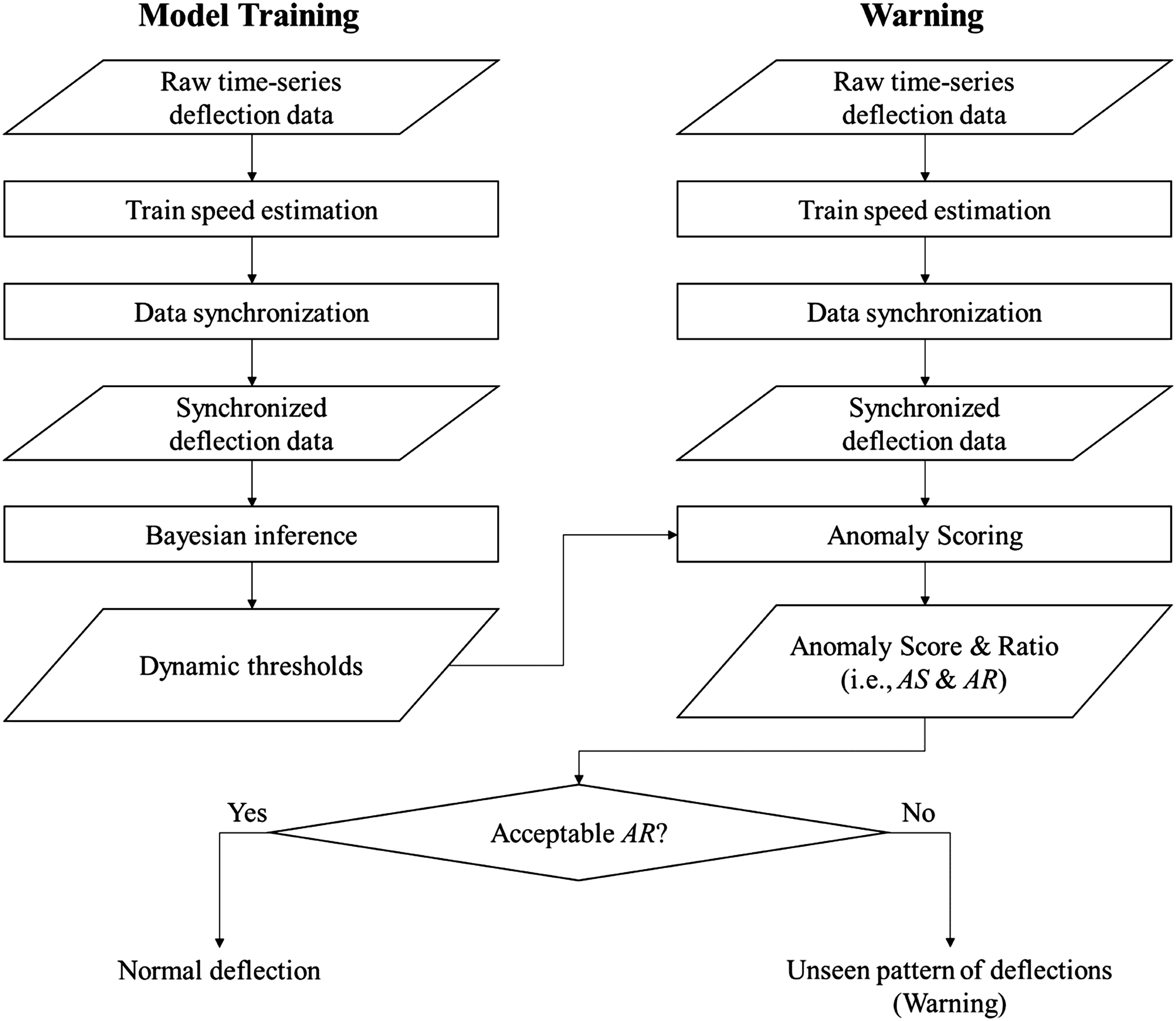

Data preprocessing of deflections subjected to various train loads

Train runs at various speeds that results different loading time elapse on passing bridge, thus, the structural responses are associated with different time intervals between entry and exit. In the proposed method, algorithms of normalizing the scale of the elapsed time were developed for the estimation of the train speed and the data synchronizing method.

Train speed estimation

Various methods for acquiring the desired train speed exist, including (1) on-board measurements via tachometers or a GPS, (2) ground measurements via optical or eddy current sensors, and (3) the speed estimation from the structural vibration measurements.²¹ In this study, the speed estimation from the structural responses was introduced because it does not require an additional train speed acquisition module in the car or field.

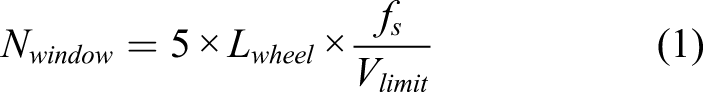
Figure 2 shows a drawing of a typical high-speed train in Korea, which consists of power car (PC), motorized trailer (MT), and passenger car. The distance between bogies is called the effective beating interval, wherein each bogie generates the downward structural deflection peaks when passing a bridge. The train speed, which is the relationship between the passing time and the length of train car, can be estimated as the effective beating interval divided by the time interval between the downward peaks in the deflection data. Based on this idea, the train speed estimation algorithm consists of three steps: (1) data windowing, (2) time interval extraction between peaks, and (3) speed estimation based on the consideration of the geometric properties of the trains.

Figure 2.

Drawing of one of a high-speed train in Korea.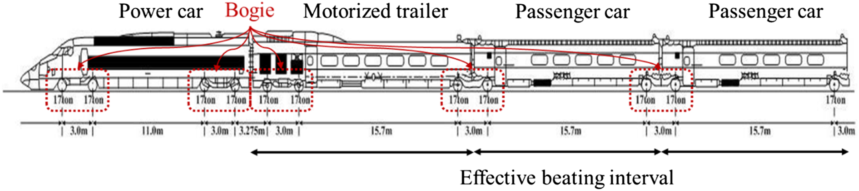

A typical structural deflection data plot is illustrated as Figure 3(a), and can be divided into two parts: unboxed and boxed regions. The bridge vibrates with its natural frequency (i.e., free vibration) before and after the train passage; this is shown in the unboxed region. The vibration shown in the boxed region is generated when the train is on the bridge, and the data windowing is a process for estimating the train speed more precisely based on the boxed region in the Figure 3(a). The first large downward deflection occurs when bogies in PC and MT (which are equipped with the heavy electric motors) passes over the bridge. The entry time can be identified by identifying the first peak point. After picking the first peak point, the data window size (i.e., N _window) can be decided by considering the sampling rate of the measurement (i.e., f _s), an admissible speed limit of the train (i.e., V _limit), and an effective beating interval length (i.e., L _wheel), as follows

N_{w i n d o w} = 5 \times L_{w h e e l} \times \frac{f_{s}}{V_{l i m i t}}

(1)

where the units of N _window, L _wheel, f _s, and V _limit are the number of samples, m, the number of samples/s, and m/s, respectively, and the number “5” was empirically determined, as it was concluded to be sufficient for estimating the speed. This means that the data window size contains the deflection data generated while first five bogies pass the measurement point. For instance, the data window extracted using this algorithm from the raw data in Figure 3(a) can be described as shown in Figure 3(b).

Figure 3.

(a) An example of time-history deflection data, and (b) extracted deflection data with data windowing.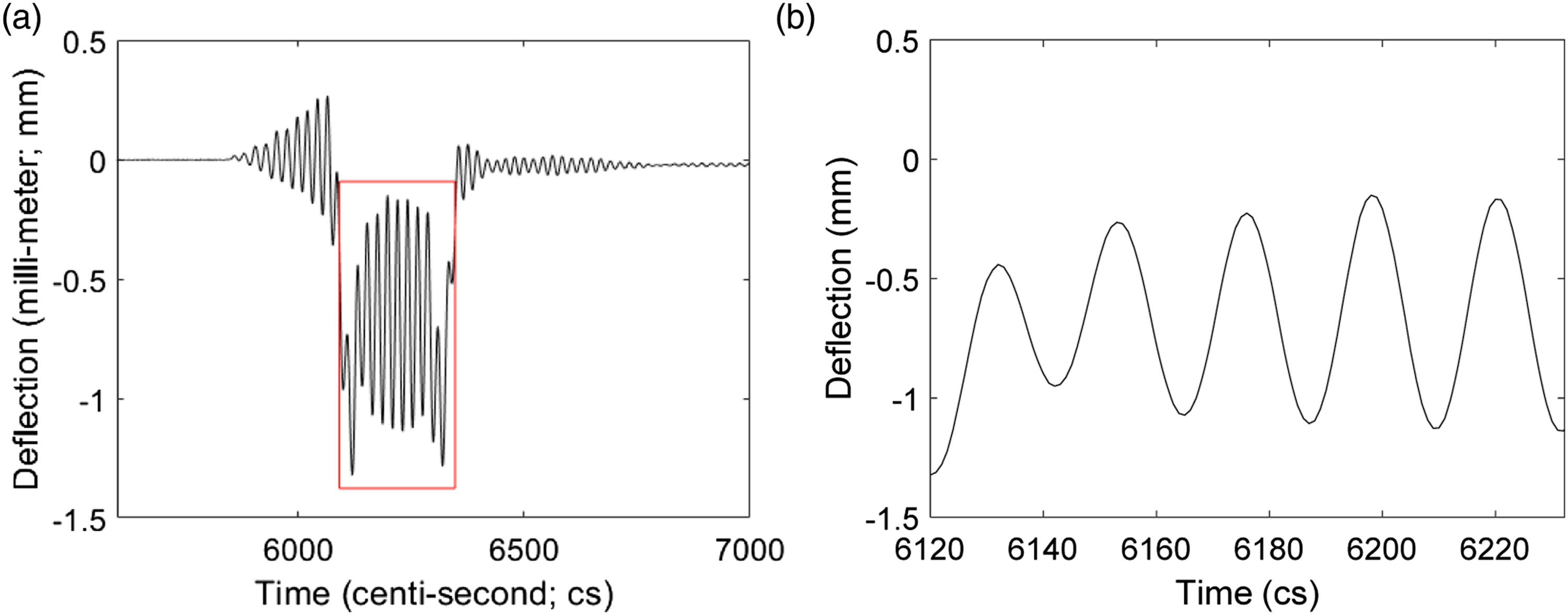

To calculate the average time interval between the downward peaks in the windowed data, various peak-picking algorithms can be introduced. In this study, a function of MATLAB with version R2020a,²² findpeak, was utilized, and the average train speed (i.e., V _train) can be estimated as follows

V_{t r a i n} = \frac{L_{w h e e l}}{Δ_{t}}

(2)

where Δ_t is the average time interval between downward peaks.

Data synchronization

The raw time-history deflection data can be plotted as shown in Figure 4(a). Herein, the two different trains of Train #1 and Train #2 have different speeds and measurement start times. To use both sensor data in training, data synchronization is required in terms of the timescale. Here, the deflection generated when the train is on the bridge is the synchronization target (i.e., the free vibration is not considered). First, as shown in Figure 4(a), the time intervals of the larger deflections occurred by the bogies between the PC and the MT of Trains #1 and #2 are 214 (i.e., 6261−6047) and 200 (i.e., 6320−6120), respectively. Herein, the timescale can be normalized by a dimensional transformation from the Time to the Location Index. By multiplying the average train speed, which can be estimated using the algorithm introduced in Train speed estimation, with time, the unit of the inputs is changed from the timescale to the location scale, as shown in Figure 4(b). The differences of the Location Index for larger deflections from PC and MT were the same and equal to 60,000 (i.e., 1,756,000−1,696,000 and 1,905,000−1,845,000). Now, the new input, Location Index, denotes an index for a specific location within the passing train which is exactly located on the sensor. Second, the timing can be synchronized based on the first downward peak point, by simply defining the Relative Location Index as the original Location Index minus the Location Index of each first peak point. As shown in Figure 4(c), the initial timing associated with the train’s entry can be matched by this idea.

Figure 4.

(a) Raw time-history deflection measurements of two trains, (b) result of dimensional transformation from the time to the location index, and (c) synchronized data.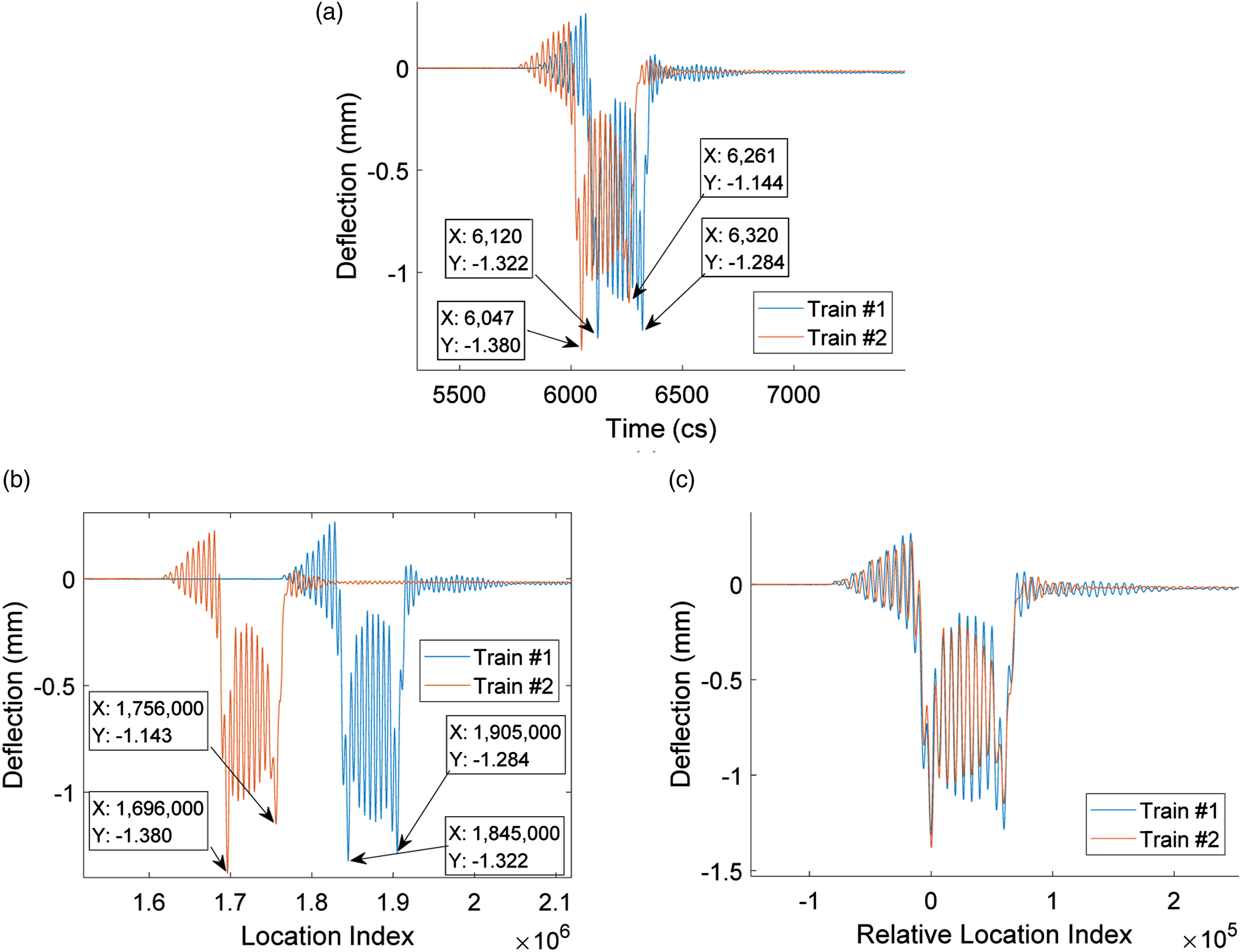

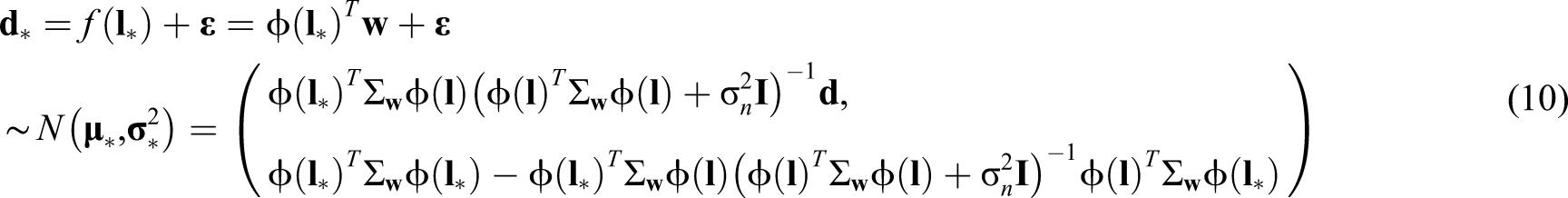
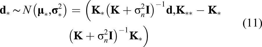
Bayesian inference for constructing dynamic thresholds

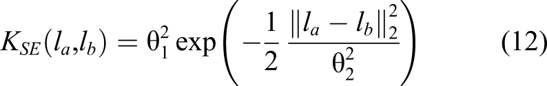
A dynamic threshold for the probabilistic detection of unseen patterns of deflections is constructed by Gaussian process regression (GPR). The Gaussian process (GP) is one of random processes in which every dataset is assumed to follow multivariate Gaussian distribution, and GPR is a probability regression method based on this GP assumption.¹⁸ It is also known as kriging, one of the well-developed interpolation methods, which requires a careful data preprocessing. The GPR was successfully applied in previous studies to construct the probabilistic prediction models of bridge deflections and structural characteristics,^17,23 and the dynamic thresholds are derived by the Bayesian inference method based on the preprocessed (i.e., synchronized) data using the methods described in Data preprocessing of deflections subjected to various train loads.

Let the matrix of the synchronized deflection data, D, which consists of two vectors for the relative location index and the deflection of l and d, be given as

D = {(l, d)} = {(l_{i}, d_{i}) | i = 1, K, N_{D}}

(3)

where l _i and d _i denote the data points whose vector sizes are N _D × 1. Herein, the relative location index and the deflection data can be expressed by the following equation

d = f (l) + ε = ϕ {(l)}^{T} w + ε

(4)

where f (·) is a regression function which is estimated as the dot product of the projection function (i.e., ϕ(·)) outputs and the weight vector (i.e., w). For example, the two-dimensional polynomial regression function can be derived by the projection function ϕ(z) = [1, z, z ²]^T and the weight vector w = [w ₁, w ₂, w ₃]^T. In this case, ε is a vector of observational errors whose size is N _D × 1, wherein the errors are assumed as a homoscedastic noise with a constant standard deviation of σ_n.

The target variables for the Bayesian inference are the elements of the weight vector w. The prior assumption on the weight vector is

w \sim N (O, Σ_{w})

(5)

where N(O, Σ _w) refers the multivariate normal distribution with a zero mean vector and a covariance matrix Σ _w. The likelihood function can be considered as the multiplication of normal probability density functions owing to the assumption of having the homoscedastic noise

p (d | l, w) = \prod_{i = 1}^{N_{D}} p (d_{i} | ϕ {(l_{i})}^{T} w) = \frac{1}{{(2 π σ_{n}^{2})}^{0.5 N_{D}}} \exp (- \frac{1}{2 σ_{n}^{2}} {‖ d - ϕ {(l)}^{T} w ‖}_{2}^{2})

(6)

where ||·||₂ is the L2 norm (i.e., the Euclidean distance). Based on the Bayes’ rule, the posterior probability is proportional to the multiplication of prior and likelihood functions; thus, it is expressed as the multiplication of two multivariate Gaussian probability density functions as follows

p (w | l, d) \propto \exp (- \frac{1}{2} w^{T} Σ_{w}^{- 1} w) \exp (- \frac{1}{2 σ_{n}^{2}} {(d - ϕ {(l)}^{T} w)}^{T} (d - ϕ {(l)}^{T} w))

(7)

which means that

p (w | l, d) \propto \exp (- \frac{1}{2} {[w - \bar{w}]}^{T} (σ_{n}^{- 2} ϕ (l) ϕ {(l)}^{T} + Σ_{w}^{- 1}) [w - \bar{w}])

(8)

where

\bar{w} = σ_{n}^{- 2} {(σ_{n}^{- 2} ϕ (l) ϕ {(l)}^{T} + Σ_{w}^{- 1})}^{- 1} ϕ (l) d

(9)

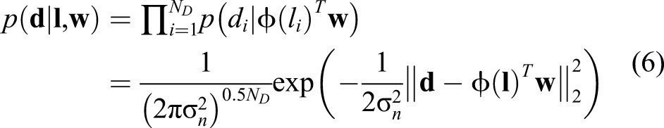
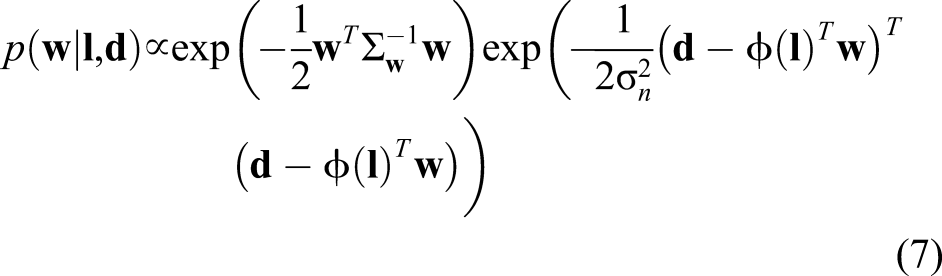
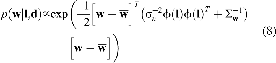
Equation (8) denotes the weight vector which follows the multivariate normal distribution with a mean vector of $\bar{w}$ and a covariance matrix of $σ_{n}^{- 2} ϕ (l) ϕ {(l)}^{T} + Σ_{w}^{- 1}$ . Therefore, the predictive mean (i.e., μ*) and standard deviation (i.e., σ*) of the deflection data for a given vector of the relative location index (i.e., l*) can be inferred as follows

\begin{array}{l} d_{*} = f (l_{*}) + ε = ϕ {(l_{*})}^{T} w + ε \\ \sim N (μ_{*}, σ_{*}^{2}) = (\begin{array}{l} ϕ {(l_{*})}^{T} Σ_{w} ϕ (l) {(ϕ {(l)}^{T} Σ_{w} ϕ (l) + σ_{n}^{2} I)}^{- 1} d, \\ ϕ {(l_{*})}^{T} Σ_{w} ϕ (l_{*}) - ϕ {(l_{*})}^{T} Σ_{w} ϕ (l) {(ϕ {(l)}^{T} Σ_{w} ϕ (l) + σ_{n}^{2} I)}^{- 1} ϕ {(l)}^{T} Σ_{w} ϕ (l_{*}) \end{array}) \end{array}

(10)

In the GPR, the term $ϕ {(\cdot)}^{T} Σ_{w}^{- 1} ϕ (\cdot)$ , which is the covariance matrix of the projected inputs, is defined by introducing kernels. When the covariance matrix estimated by kernels is expressed by the capital letter K, Equation (10) can be expressed by substituting the covariance matrix of the projected inputs into K as follows

d_{*} \sim N (μ_{*}, σ_{*}^{2}) = (Κ_{*} {(Κ + σ_{n}^{2} I)}^{- 1} d, Κ_{* *} - Κ_{*} {(Κ + σ_{n}^{2} I)}^{- 1} Κ_{*})

(11)

Various kernel functions have been developed to numerically describe the covariance terms (i.e., K, K*, and K**), which can be categorized in two groups, namely, for stationary and nonstationary patterns. For stationary data wherein the correlation decreases a function of the distance between the data, the stationary kernels can be introduced; by contrast, the nonstationary data require the kernel that contains the nonstationary terms, which is not a decreasing function with respect to distance. For example, the squared exponential kernel (K _SE) is one of the kernels used for the stationary data as follows

K_{S E} (l_{a}, l_{b}) = θ_{1}^{2} \exp (- \frac{1}{2} \frac{{‖ l_{a} - l_{b} ‖}_{2}^{2}}{θ_{2}^{2}})

(12)

where θ₁ and θ₂ are the hyperparameters which need to be optimized, whereas the periodic kernel (K _PER) is one of the kernels used for the nonstationary data

K_{P E R} (l_{a}, l_{b}) = θ_{1}^{2} \exp (- \frac{2 \sin (π {‖ l_{a} - l_{b} ‖}_{2}^{2} / p)}{θ_{2}^{2}})

(13)

where p is the period. Once the kernel is determined, the hyperparameters can be optimized through the minimization of the minus log-marginal likelihood (L) as follows

L = - \ln p (d | l) = \frac{1}{2} d^{T} {(Κ + σ_{n}^{2} I)}^{- 1} d + \frac{1}{2} \ln | Κ + σ_{n}^{2} I | + \frac{N_{D}}{2} \ln (2 π)

(14)

The Gaussian process regression is introduced in this study owing to two advantages: (1) its flexibility in constructing a nonlinear function without the need to predetermine the functional order, and (2) its ability to quantify the uncertainties in the given data. First, the time-history deflections of railway bridges induced by high-speed trains have complex data patterns; these would ordinarily be fitted by high-order functions. However, it is not easy to decide the appropriate functional order to fit a deflection pattern; thus, the Gaussian process regression, a nonparametric method, is utilized to avoid the need to predetermine the functional order. Second, the magnitudes of the deflections are probabilistic because those are affected by not only the structural conditions (e.g., material properties), but also by the weights and speeds of trains and the environmental conditions (e.g., temperature), which are probabilistic. Thus, the Gaussian process regression was introduced to quantify the probabilistic range of deflections.

Anomaly scoring method

The dynamic thresholds of deflections for given relative location indices can be derived by the Bayesian inference using equations (10) and (11). Once this probabilistic monitoring model is constructed, the detection of the unusual deflections can be conducted. First, the given time-history raw data needs to be preprocessed as introduced in data preprocessing of deflections subjected to various train load, and an anomaly score of the given synchronized data is estimated. Herein, the term, anomaly denotes a strange condition that has a noticeable deviation from the normal state, which can be either the abnormal or normal conditions which were not or rarely detected before.

Proposed indices for estimating the amount of the anomalies in the measured deflection data are the Anomaly Score (AS) and Anomaly Ratio (AR). Let the predictive mean and standard deviation for the given relative location index be μ_l and σ_l. The AS of the deflection (i.e., d _l) for the given relative location index is then defined as the Boolean logic as follows

A S (d_{l}) = {\begin{matrix} 1, for Φ (\frac{| d_{l} - μ_{l} |}{σ_{l}}) > \frac{1 + p_{t h r e s h o l d}}{2} \\ 0, for Φ (\frac{| d_{l} - μ_{l} |}{σ_{l}}) \leq \frac{1 + p_{t h r e s h o l d}}{2} \end{matrix}

(15)

where Ф(·) denotes a cumulative distribution function value of a standard normal distribution, and p _threshold is a threshold probability that needs to be decided. For example, if the anomaly deflection is expected to exceed the 95% margin of the probabilistic prediction range, the p _threshold can be chosen to be 0.95.

The AR index is calculated as the sum of the AS divided by the total number of measurements, which denotes the ratio of the anomalies among all the samples. Herein, the start and end points of the measured data are defined as the train’s entry and exit times, as shown in Figure 5, because the AR index is affected by the range of the measured data (e.g., longer range would decrease the AR index, even though the train causes the same number of anomalies). When the AR index is larger than 1− p _threshold, the deflections are considered as unseen patterns (i.e., unacceptable level of AR) and require warnings.

Figure 5.

(a) Original and (b) target ranges of the deflection data.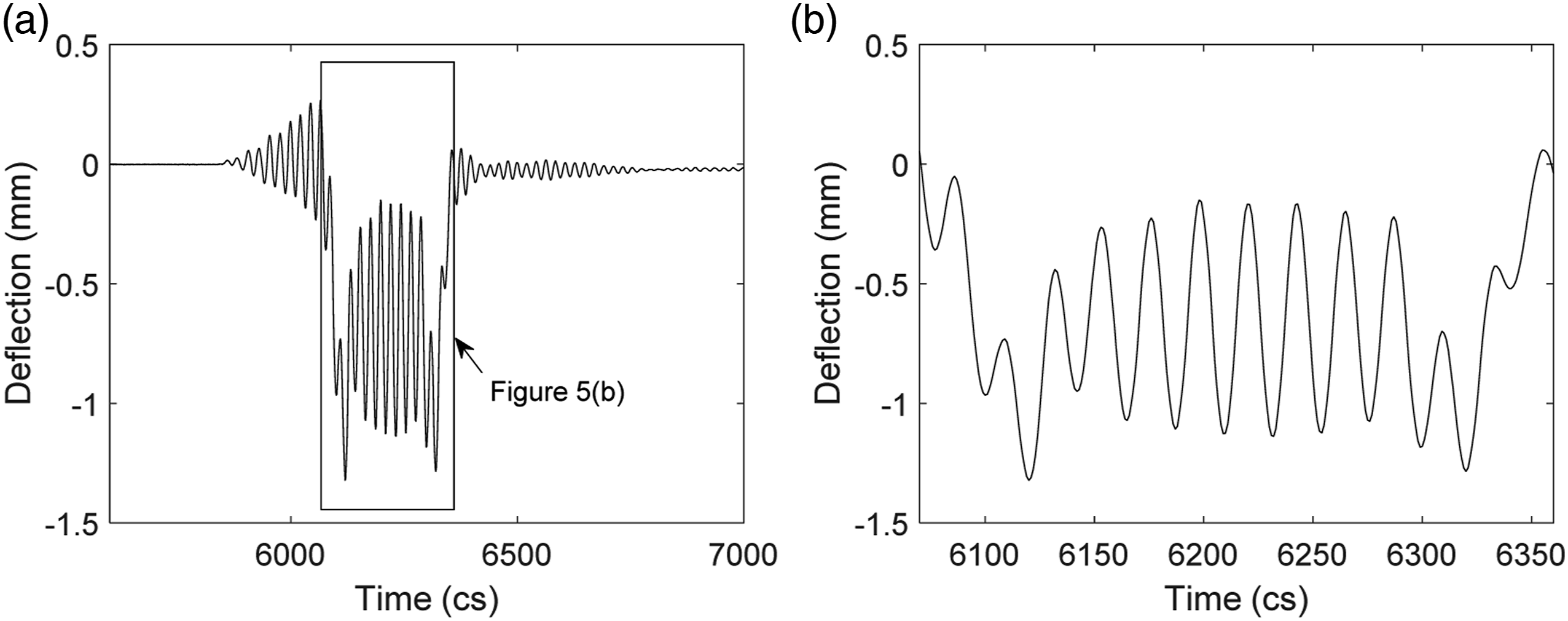

Field application example

Target bridge and measured data

The proposed method was applied to a prestressed concrete railway bridge located in the Republic of Korea wherein several types of high-speed trains pass through, such as the Korea Train eXpress (i.e., KTX) and the Super Rapid Train (i.e., SRT). Three types of high-speed trains pass over the bridge: a single unit train with 10 cars, a single unit train with 20 cars, and coupled units train with two ten-cars (i.e., 20 cars in total), as shown in Figure 6. These are called ten-car, twenty-car, and twenty-car with coupled ten-cars types, respectively, in this paper. The PCs and MTs are heavier than other cars and highlighted in blue and red in the Figure 6. The ten-car and twenty-car types have the PC and the MT at both ends, but the twenty-car with coupled ten-cars types have two sets of the PC and the MT at both ends and a double-set of the PC and the MT at the middle. Therefore, the deflection patterns are distinct for each type.

Figure 6.

Three types of the high-speed trains that pass through the example bridge: (a) ten-car type, (b) twenty-car type, and (c) twenty-car with coupled ten-cars type.

The vertical deflection of the bridge was measured by the LVDT sensor at the midspan of the main girder. Totally 312 number of time-history deflection data (157, 41, and 114 for the ten-car type, twenty-car type, and twenty-car with coupled ten-cars type, respectively) were collected for 3.5 days from September 3rd 13:06 to September 6^th 23:52, 2020. As shown in Figures 7(a) and (b), the deflections attributed to the ten-car and the twenty-car types have big major peaks (circled in red) of downward deflection at both ends, whereas the deflection which occurred by the twenty-car with coupled ten-cars type has two major peaks at both ends and additional major peak in the middle. Because the ten-car type is shorter than others, the time needed to pass through the bridge is shorter than others, as described in Figure 7. In addition, as the location at which the vertical deflection is measured is close to the abutment, the trains coming from the abutment side rarely occur the free vibration before passage, as shown in the first part of Figure 7(c). On the other hand, when a train comes from the other side, the bridge experiences the vibrations shown in Figures 7(a) and (b), owing to the vibrations of neighboring bridges. The train speeds can be estimated from the measured data and the effective beating interval (18.7 m for all high-speed trains in Korea), as introduced in train speed estimation, and the range was between 228.2 km/h to 328.4 km/h.

Figure 7.

Deflection patterns of (a) ten-car type, (b) twenty-car type, and (c) twenty-car with coupled ten-cars type.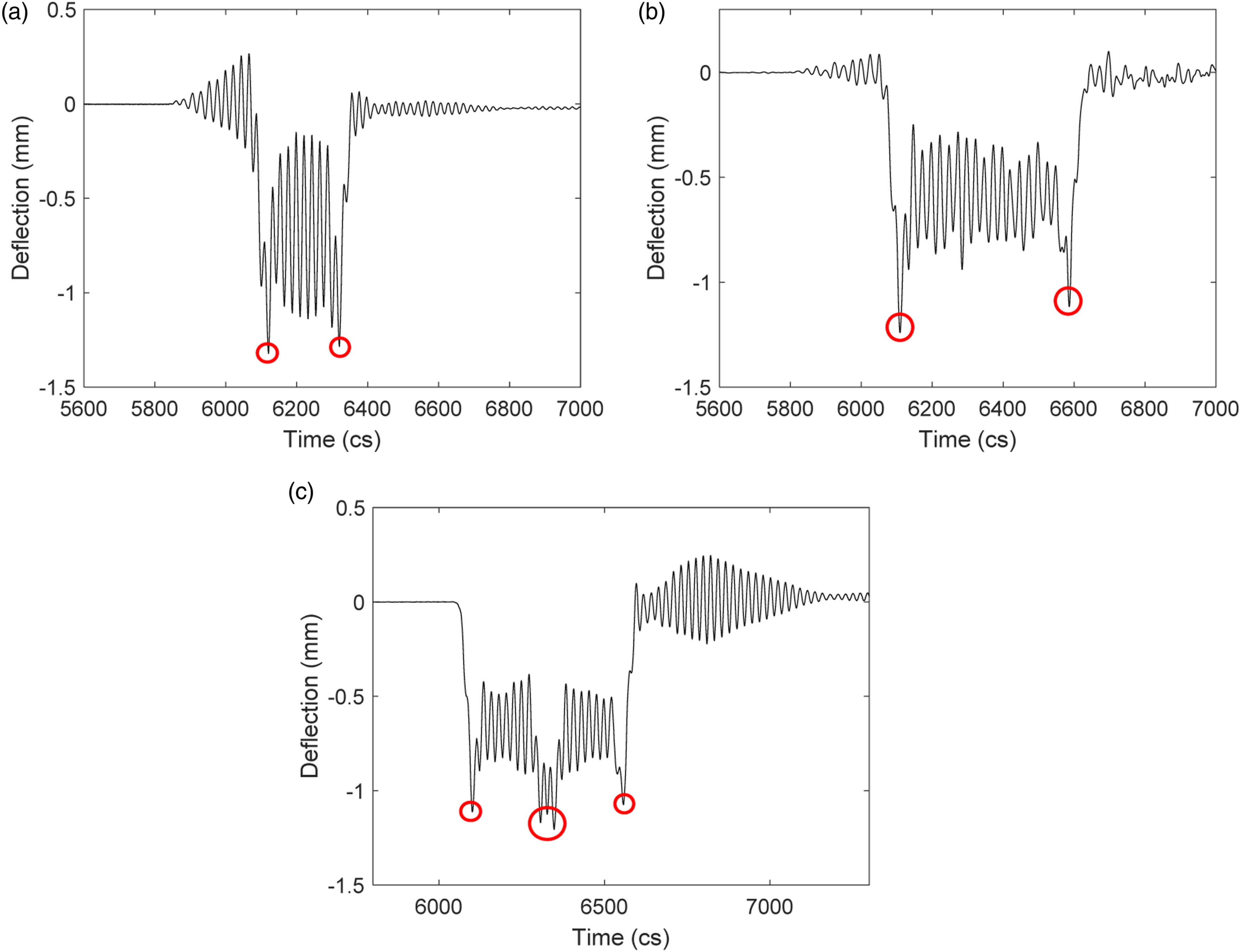

Probabilistic deflection monitoring for example bridge

The probabilistic monitoring models for train types generating different data patterns of deflection were constructed using three quarters of the measured data (i.e., 117, 31, and 86 for the ten-car type, twenty-car type, and twenty-car with coupled ten-car type, respectively), as shown in Figure 8. Black solid lines are the predictive mean and the dotted lines are 99% prediction interval (i.e., p _threshold = 0.99) for the given relative location index. Notably, other factors, such as the material properties, the weights of trains and environmental conditions, only affect the magnitude of the deflection; they were considered as the uncertainty factors. As described in probabilistic deflection monitoring of high-speed railway bridge, the train speed estimation and data synchronization are conducted to obtain the deflection data given the relative location index. The AS and AR values can thus be estimated with equation (14). If the AR is smaller than 0.01 (i.e., 1 - p _threshold), this can be considered as a normal state; in contrast, a problem in the structural component or trains may be expected if the AR is larger than 0.01.

Figure 8.

Probabilistic deflection monitoring models for (a) ten-car type, (b) twenty-car type, and (c) twenty-car with coupled ten-car type.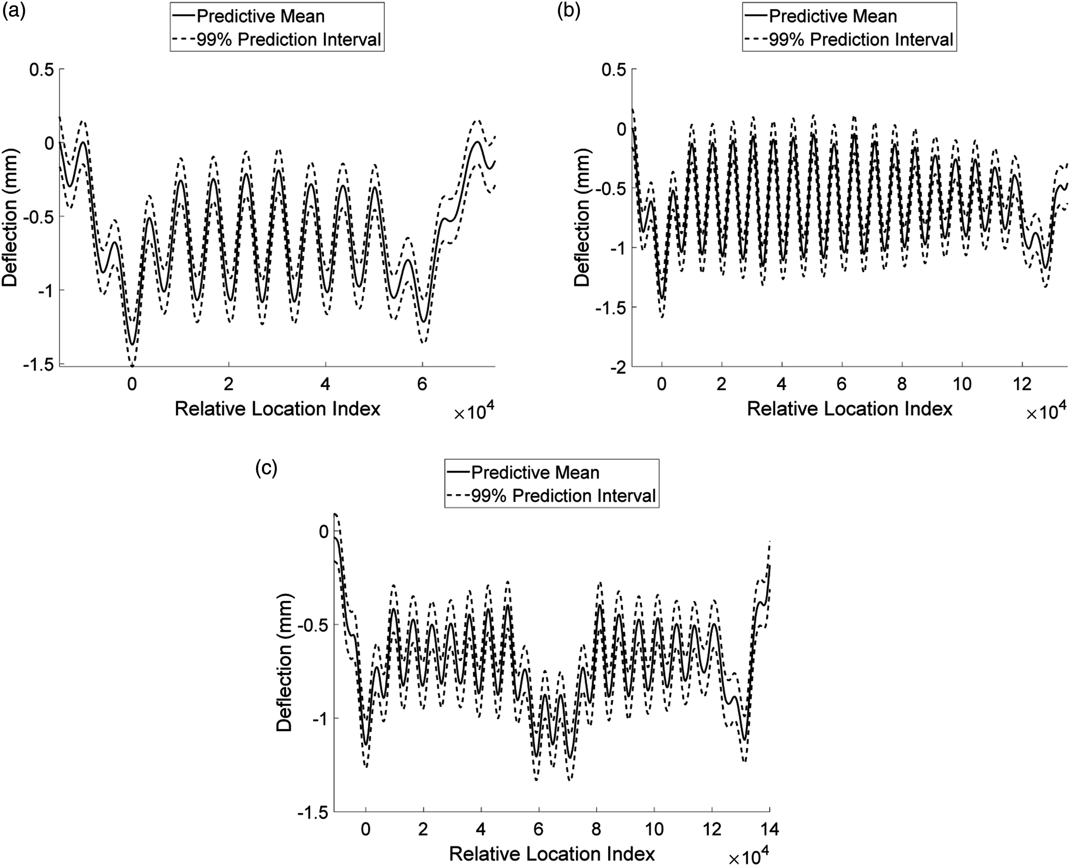

Figure 9 shows the examples of estimating the AS and AR based on the probabilistic deflection monitoring models for each of the three train types. Those were calculated for the two sets of actual deflection data measured from the example bridge, which were not introduced in the training. As shown in Figure 9, the AR was estimated to be smaller than 0.01 (e.g., 0.000 and 0.003 in Figure 9(a), 0.000 and 0.004 in Figure 9(b), and 0.000 and 0.000 in Figure 9(c)), which shows that the given deflection patterns are similar with the traning data. Therefore, in this case, the bridge and the running train are expected to operate under the normal condition.

Figure 9.

Examples of AS and AR estimations based on the probabilistic deflection monitoring models for (a) ten-car type, (b) twenty-car type, and (c) twenty-car with coupled ten-car type.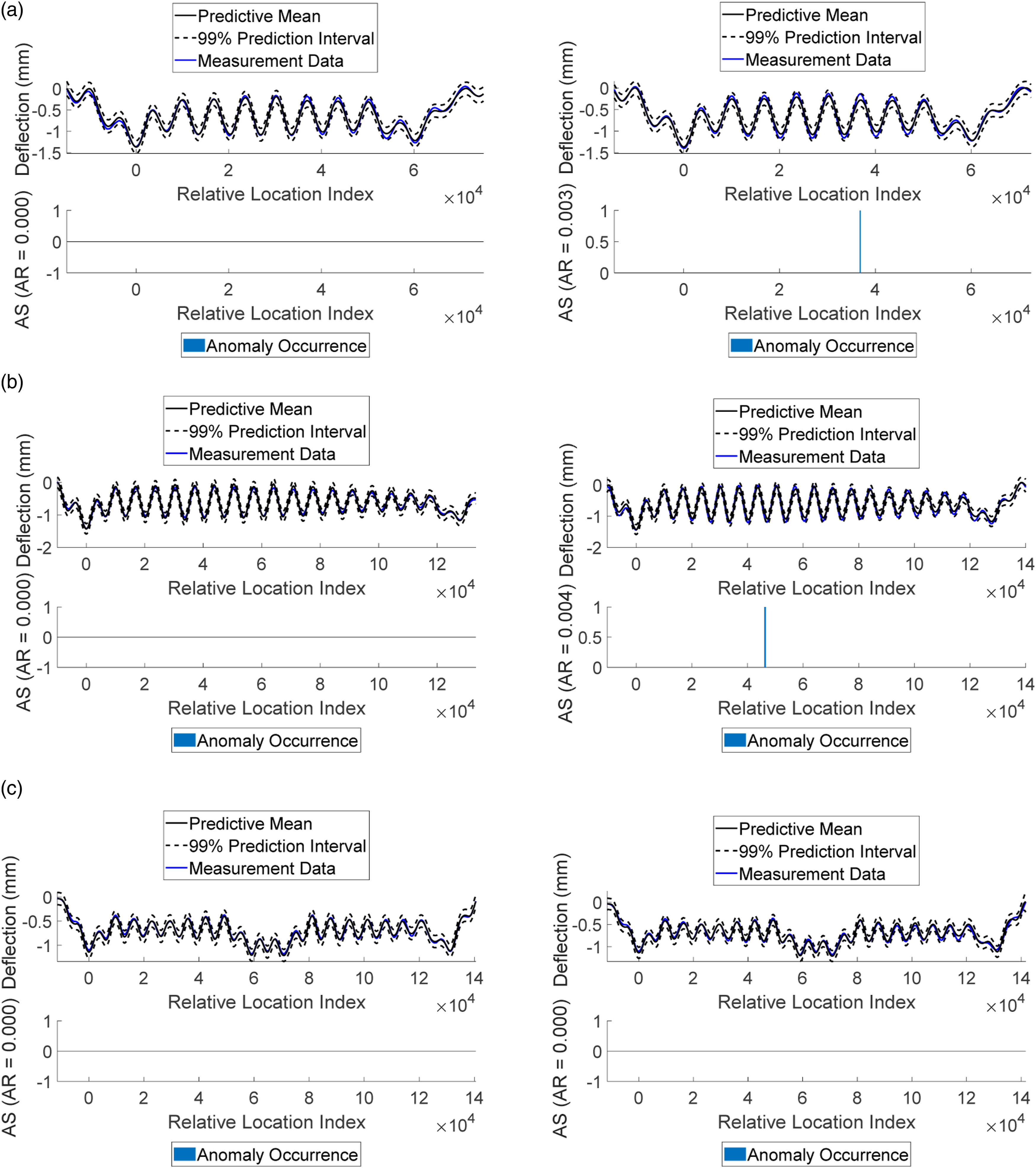

However, when the deflection patterns are abnormal (identified for large AR values), they are not under the normal condition. For instance, when a train wheel has a certain defect such as a wheel flat, a larger impact force instantly applies to the bridge and changes the deflection patterns.²⁴ The proposed monitoring model can detect this response. According to Han et al. (2017), the vertical impact force from a 20-mm wheel flat with a 250 km/h train speed and 17 ton axle load is approximately 2.6 times larger than the average static axle loads.²⁵ From this finding, the data for the abnormal deflection pattern was numerically generated. Figure 10 shows the probabilistic monitoring models and the deflections patterns with a wheel flat on a specific wheel. As described in Figure 10, the AR values of the given data for the three types were 0.023, 0.012, and 0.015, respectively, which are greater than the acceptable level of 0.01. Because these AR values are at unacceptable levels, a warning can be generated, wherein the changes of the condition of structures or trains may be expected. Especially, one may intuitively detect a local abnormality as well because the anomalous deflections appear locally. In case of Figure 10(a), the third and fourth bogies of the trains that occur at the third peak should be checked because the deflection was amplified compared to usual responses.

Figure 10.

Examples of AS and AR estimations for the deflections with the wheel flat for (a) ten-car type, (b) twenty-car type, and (c) twenty-car with coupled ten-cars type.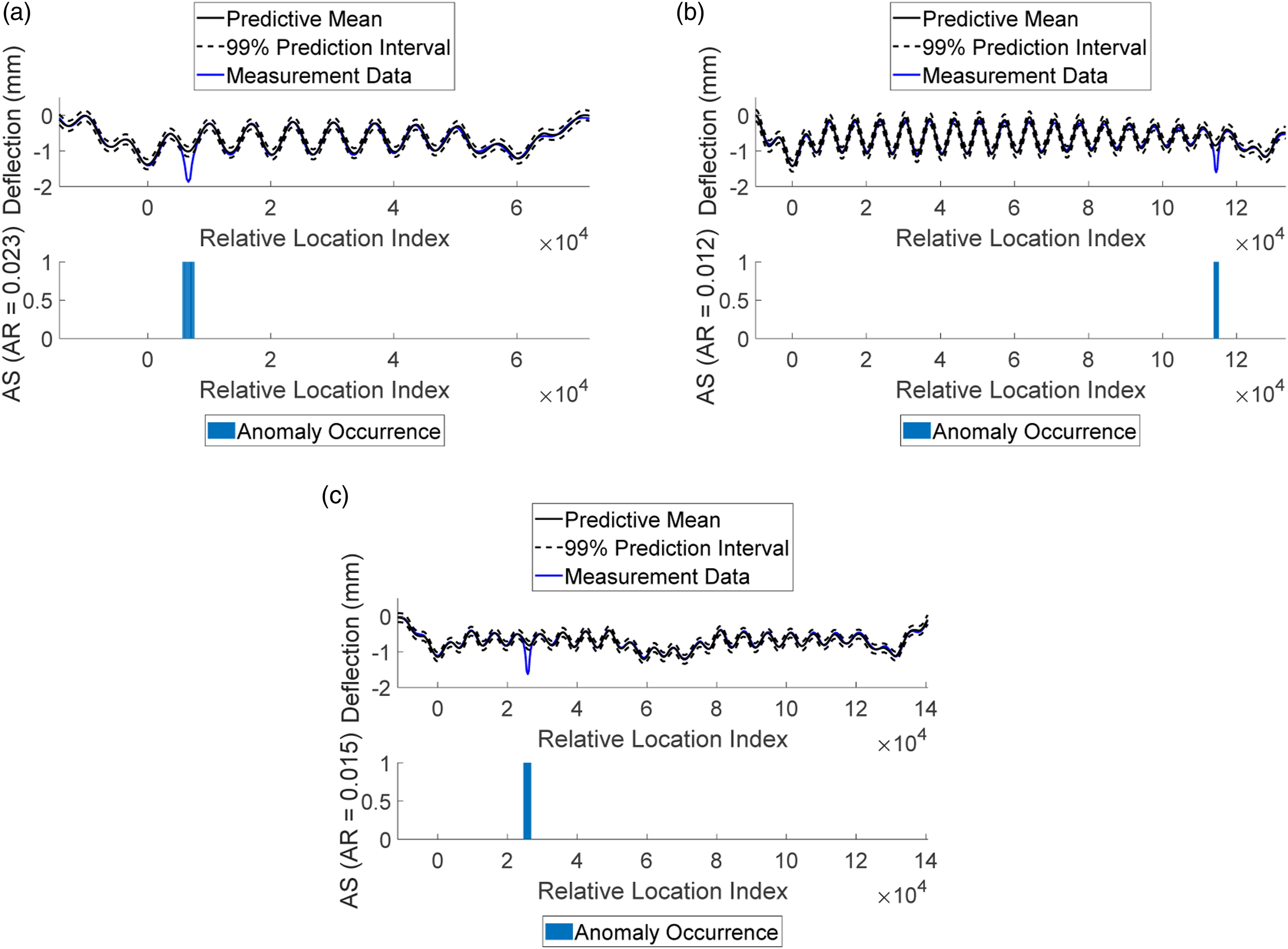

When the stiffness of a bridge structure is reduced by some damages, deflection magnitudes may increase,²⁶ which can also be detected using the proposed monitoring model. Figure 11 shows the hypothetical examples of time-history deflections with 5% increases of the midlines representing the original time-history deflections of the undamaged structure, owing to stiffness reduction. The original deflections are not constants and fluctuate with time; therefore, the amount of the 5% increase is different at each time point. As shown in the figure, the AR values of the data provided for the three types were 0.056, 0.051, and 0.062, respectively, which are greater than the acceptable level of 0.01. These may generate a warning so that and necessary actions can be adopted, such as further inspection of a bridge. Moreover, anomaly owing to the decrease in bridge stiffness is confirmed at multiple locations, which is distinguished from the result of wheel flat damage (shown in Figure 10) where anomaly occurs when a specific damaged wheel of a vehicle passes the mid-span of a bridge. In this way, the proposed method can be utilized not only for detecting anomalous signals generated owing to the abnormal structural conditions of a train-track-bridge system but also for estimating its cause by checking the locations and magnitudes of the anomalous signals.

Figure 11.

Examples of AS and AR estimations for the deflections with stiffness reduction for (a) ten-car type, (b) twenty-car type, and (c) twenty-car with coupled ten-car type.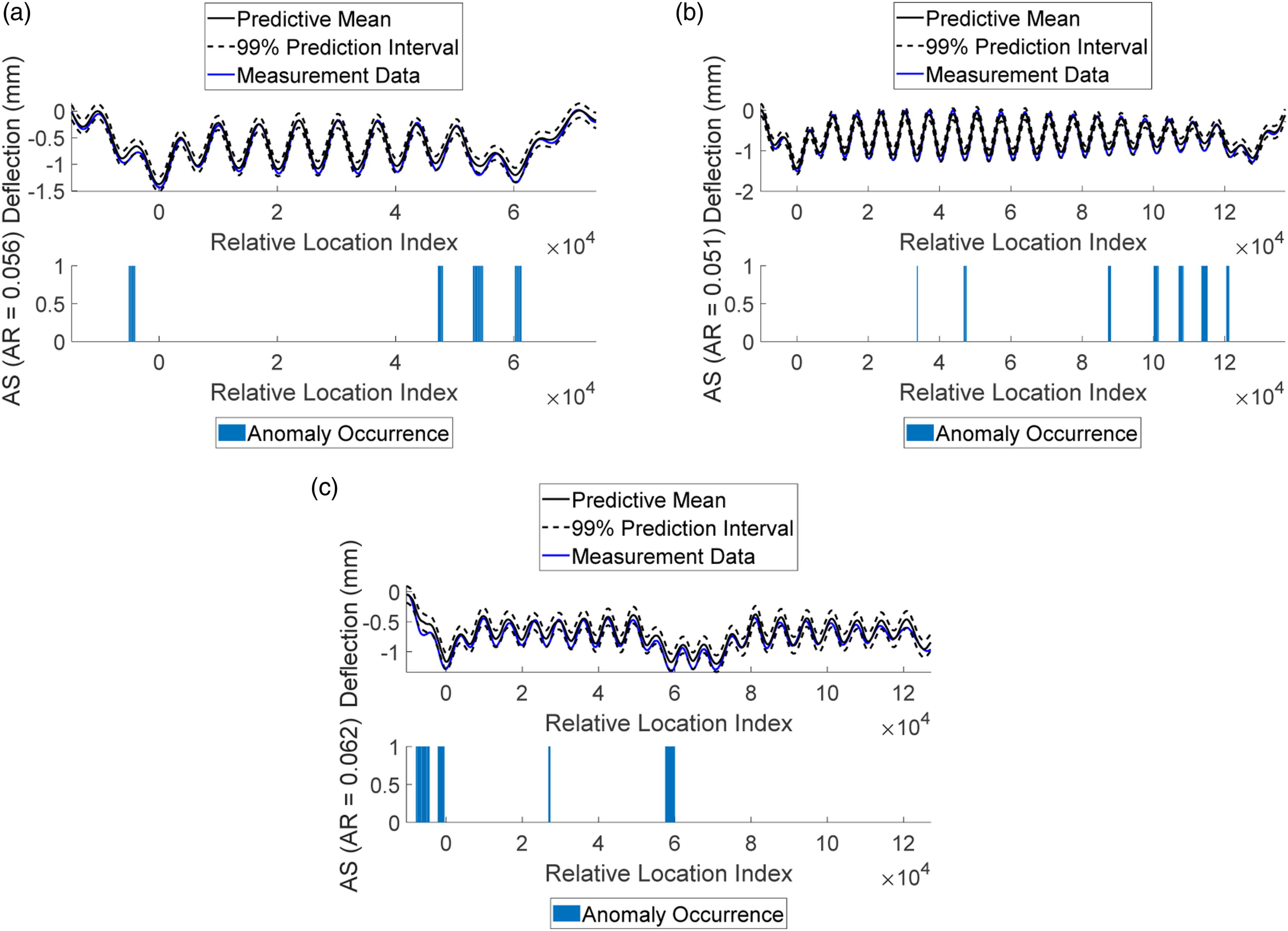

Conclusion

This study proposed a new method for the probabilistic monitoring of the time-history deflections of railway bridges induced by high-speed trains. For training the monitoring model, the data preprocessing which are the speed estimation and data synchronization are conducted first for the given raw time-history deflection data, and the Bayesian inference is then conducted for deriving the dynamic thresholds for each of the train types considered. After constructing the monitoring model, the speed estimation and data synchronization are repeated. The AS and AR indices are then estimated based on the probabilistic deflection monitoring model, and the unseen patterns of the deflection data can be detected. The warning can be generated if the AR is at an unacceptable level, whereas the structure may be considered as a normal condition if the AR is at an acceptable level. The proposed method was applied to an operating railway bridge in the Republic of Korea, and probabilistic monitoring models were constructed for the time-history deflections of the main girder. The estimated AR was smaller than the threshold if no problems existed in the structure or train, but it was found that the unusual deflection patterns attributed to anomalous conditions of a train-track-bridge system led to AR value increases at levels higher than the threshold. As discussed, the probabilistic monitoring model constructed using the proposed method can be utilized not only for detecting the occurrence of anomalous structural responses, but also for identifying their potential causes by checking the locations and magnitudes of the anomalous signals. The authors expect that the proposed method will be used for an efficient monitoring and management of the structural responses of railway bridges subject to high-speed trains.

Footnotes

Declaration of conflicting interests

The authors declared no potential conflicts of interest with respect to the research, authorship, and/or publication of this article.

Funding

The author(s) disclosed receipt of the following financial support for the research, authorship, and/or publication of this article: This research was supported by a grant (21SCIP-B138406-06) from Construction technology research program funded by Ministry of Land, Infrastructure and Transport of Korean government. This work was also supported by the National Research Foundation of Korea (NRF) grant funded by the Korea government (MSIT) (2021R1C1C2008770).

ORCID iDs

Sung-Han Sim

Young-Joo Lee

References

Ding

Y-L

Zhao

H-W

Deng

, et al. Early warning of abnormal train-induced vibrations for a steel-truss arch railway bridge: case study. J Bridge Eng 2017; 22(11): 05017011.

Zhao

H-W

Ding

Y-L

Nagarajaiah

, et al. Behavior analysis and early warning of girder deflections of a steel-truss arch railway bridge under the effects of temperature and trains: case study. J Bridge Eng 2019; 24(1): 05018013.

Guan

Ding

, et al. Fast warning method for rigid hangers in a high-speed railway arch bridge using long-term monitoring data. J Perform Constructed Facil 2017; 31(6): 04017103.

Jeon

B-G

Kim

N-S

Kim

S-I

. Estimation of the vibration serviceability deflection limit of a high-speed railway bridge considering the bridge-train interaction and travel speed. KSCE J Civil Eng 2016; 20(2): 747–761.

Kaloop

Sayed

. Yonjung high-speed railway bridge assessment using output-only structural health monitoring measurements under train speed changing. J Sensors 2016; 2016.

Ding

Sun

Wang

, et al. Early-warning method of train running safety of a high-speed railway bridge based on transverse vibration monitoring. Shock and Vibration 2015; 2015.

. Technology developments in structural health monitoring of large-scale bridges. Eng Structures 2005; 27(12): 1715–1725.

Zhou

Sun

Wei

, et al. Deflection-based multilevel structural condition assessment of long-span prestressed concrete girder bridges using a connected pipe system. Measurement 2021; 169: 108352.

Korea Rail Network Authority . Guideline of Track Maintenance. Daejeon, Korea: Korea Rail Network Authority, 2016.

10.

Vagnoli

Remenyte-Prescott

Andrews

. Railway bridge structural health monitoring and fault detection: State-of-the-art methods and future challenges. Struct Health Monit 2018; 17(4): 971–1007.

11.

Fan

Huang

Ren

, et al. Real-time dynamic warning on deflection abnormity of cable-stayed bridges considering operational environment variations. J Performance Constructed Facilities 2021; 35(1): 04020123.

12.

Han

Xiang

T-Y

Xie

H-B

. A Bayesian inference framework for predicting the long-term deflection of concrete structures caused by creep and shrinkage. Eng Structures 2017; 142: 46–55.

13.

Avendaño-Valencia

Chatzi

Koo

, et al. Gaussian process time-series models for structures under operational variability. Front Built Environ 2017; 3: 69.

14.

Talaei

Beitollahi

Moshirabadi

, et al. Vibration-based structural damage detection using twin Gaussian process (TGP). In: Structures, 16. Elsevier; 2018, pp. 10–19.Structures

15.

Zhang

Rogers

Cross

. Gaussian process based grey-box modelling for shm of structures under fluctuating environmental conditions. In: European Workshop in Structural Health Monitoring . Cham: Springer; 2020, pp. 55–66.

16.

Salcher

Pradlwarter

Adam

. Reliability assessment of railway bridges subjected to high-speed trains considering the effects of seasonal temperature changes. Eng Structures 2016; 126: 712–724.

17.

Lee

K-C

Lee

Y-J

. Long-term deflection prediction from computer vision-measured data history for high-speed railway bridges. Sensors 2018; 18(5): 1488.

18.

Lee

K-C

Sim

S-H

, et al. Bayesian Prediction of Pre-Stressed Concrete Bridge Deflection Using Finite Element Analysis. Sensors 2019; 19(22): 4956.

19.

Lee

K-C

Jeong

, et al. Long-term displacement measurement of full-scale bridges using camera ego-motion compensation. Mech Syst Signal Process 2020; 140: 106651.

20.

Cao

Zhang

Bertola

, et al. Time Series Data Interpretation for ‘wheel-Flat’ Identification Including Uncertainties. Structural Health Monitoring, 2019, p. 1475921719887117.

21.

Wang

Shi

Wang

, et al. Train speed estimation from track structure vibration measurements. Appl Sci 2020; 10(14): 4742.

22.

MATLAB . Version R2020a. Natick, MA: The MathWorks Inc, 2020.

23.

Lee

Y-J

Shim

C-S

. Probabilistic prediction of mechanical characteristics of corroded strands. Eng Structures 2020; 203: 109882.

24.

Lee

Chiu

. Determination of railway vertical wheel impact magnitudes: Field trials. Struct Health Monit 2007; 6(1): 49–65.

25.

Han

Jing

Liu

. A dynamic simulation of the wheel-rail impact caused by a wheel flat using a 3-D rolling contact model. J Mod Transportation 2017; 25(2): 124–131.

26.

Feng

. Model updating of railway bridge using in situ dynamic displacement measurement under trainloads. J Bridge Eng 2015; 20(12): 04015019.

Sensor data-based probabilistic monitoring of time-history deflections of railway bridges induced by high-speed trains

Abstract

Keywords

Introduction

Probabilistic deflection monitoring of high-speed railway bridge

Data preprocessing of deflections subjected to various train loads

Train speed estimation

Data synchronization

Bayesian inference for constructing dynamic thresholds

Anomaly scoring method

Field application example

Target bridge and measured data

Probabilistic deflection monitoring for example bridge

Conclusion

Footnotes

Declaration of conflicting interests

Funding

ORCID iDs

References