
Abstract
The successful implementation of Structural Health Monitoring (SHM) systems is confined to the capability of evaluating their performance, reliability, and durability. Although there are many SHM techniques capable of detecting, locating and quantifying damage in several types of structures, their certification process is still limited. Despite the effort of academia and industry in defining methodologies for the performance assessment of such systems in recent years, many challenges remain to be solved. Methodologies used in Non-Destructive Evaluation (NDE) have been taken as a starting point to develop the required metrics for SHM, such as Probability of Detection (POD) curves. However, the transposition of such methodologies to SHM is anything but straightforward because additional factors should be considered. The time dependency of the data, the larger amount of variability sources and the complexity of the structures to be monitored exacerbate/aggravate the existing challenges, suggesting that much work has still to be done in SHM. The article focuses on the current challenges and barriers preventing the development of proper reliability metrics for SHM, analyzing the main differences with respect to POD methodologies for NDE. It was found that the development of POD curves for SHM systems requires a higher level of statistical expertise and their use in the literature is still limited to few studies. Finally, the discussion extends beyond POD curves towards new metrics such as Probability of Localization (POL) and Probability of Sizing (POS) curves, reflecting the diagnosis paradigm of SHM.
Keywords
Introduction
The concept of inspection is fundamentally different from the concept of monitoring according to Derriso et al. in three main aspects: the evaluation frequency, the use of previous system outcomes, and the decision range which is possible exploiting the evaluation process results. 1 Therefore, while inspections are conceived to provide a go/no go evaluation related to the health of a structural component, monitoring offers the possibility to take multiple actions thanks to the higher amount of available information.
Farrar and Worden defined SHM as the process of implementing a damage identification strategy for aerospace, civil and mechanical engineering infrastructure. 2 Other definitions are available in the literature, 3–6 all have the common goal of switching from the current scheduled maintenance philosophy to a condition-based maintenance approach.
Condition-based maintenance empowered by SHM can reduce maintenance costs, inspection time 7 and downtime. 4 The reduced labor requirement of SHM can lead to an increase in safety 4,8 compared to manual inspections, not only for the personnel, but also for the structure itself which may be accidentally damaged during inspections. 9 For difficult-to-reach area, SHM offers the possibility to overcome the accessibility limitations by permanently installed sensors. 10 The military industry sees SHM as an opportunity to increase the combat asset readiness. 11 The examples of other benefits of SHM are the early detection of damage during normal operational conditions and a drastic decrease of the human factor. 7
In the recent years, the usage of composites has been increasing. However, the complexity of such materials and the presence of a multitude of different possible damage mechanisms still force engineers to use a conservative design approach. 6 The availability of online monitoring data provided by the SHM may enhance the understanding of the new materials and thus leave room to more innovative and closer-to-the-limit design. The reduction of structural design margins can lead to lighter structures. If the structural weight reduction is higher than the additional weight of the monitoring system (sensors, cables, and electronics), lower fuel consumption thus lower CO2 emissions as well as wider design range are expected. 4
A Sandia National Labs report written by Roach in 2011 stated that the Technology Readiness Level (TRL) of SHM systems did not go beyond TRL 8 and the majority were concentrated at TRL 4. 12 In 2013 Seaver et al. 13 presented a classification of different sensing technologies based on their TRL. At that time, the TRL was ranging from 3 to 9 depending on the specific application. In recent years, several technologies based on ultrasonic permanently installed sensors such as guided wave monitoring and point thickness measurements became commercially successful. 14 However, there are still barriers preventing a complete transition toward SHM. In 2018 Cawley addressed the main reasons of this unsatisfying rate of transition from NDE towards practical applications of SHM. 14 The lack of specific techniques for performance validation, regarding both damage detection and its corresponding false call rate, was identified as a critical point preventing the widespread of SHM. The need of performance validation was also outlined in a recent publication of the same author. 15 The MIL-HKBK-1823A 16 allows the assessment of NDE methods exploiting the concept of Probability of Detection (POD) curves. However, there is a lack of specific guidelines and procedures to evaluate the system monitoring capabilities in the field of SHM. 9
The awareness in the SHM community about the topic of POD curves is still limited. Figure 1 shows the number of publications with the keywords “SHM” and “SHM+POD” since 1995. Despite increasing attention to SHM, only few studies were related to POD curves. Trend of the keywords “SHM” and “SHM+POD” analyzing the publications selected from Web of Science Core Collection (May 2021).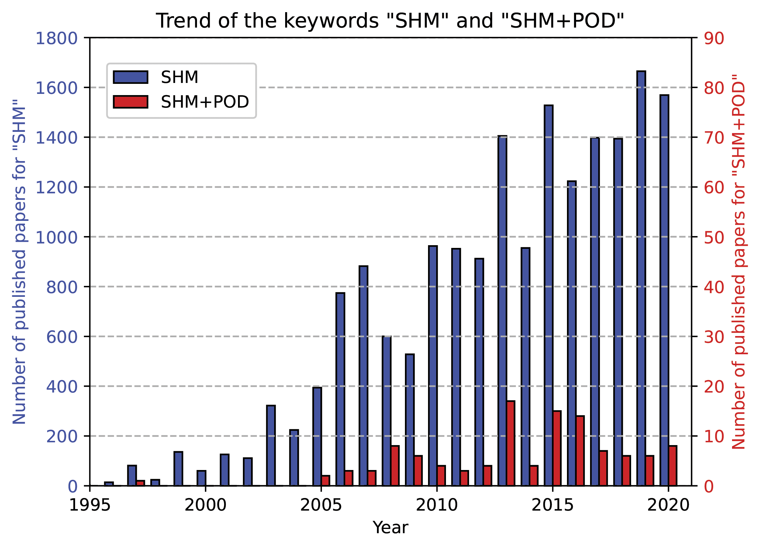
The establishment of common certification criteria is fundamental to the application of SHM technologies, 17–21 and has the potential of improving the design of the system itself. 22 According to Aldrin et al. the qualification of SHM technologies should be based on already present guidelines, 23 such as: cost–benefit analysis (CBA), 24 materials and structure certification, NDE metrics (i.e., POD curves), 16 and procedures for performing a Failure Mode, Effects, and Criticality Analysis (FMECA). 25 In 2011 Aldrin et at. Formulated a protocol, 26 mainly based on the already existing MIL-HKBK-1823A. 16 One year later, this protocol was applied to a real case study, with promising results. 18 Kessler examined three validation standards, 27–29 already utilized in the aeronautical sector, in an attempt of identifying potential relationships with SHM applications. 30
The scientific question arising from these preliminary considerations is when it is possible to apply standard POD curves for SHM systems. SHM systems can be classified in four categories. 31 First, it is possible to distinguish scheduled SHM (S-SHM) systems, from automatic SHM (A-SHM). 3 In this case the classification is done according to the way sensor data are collected, scheduled time intervals in the former and continuously in the latter. Second, the damage location can be known (KDL) or unknown (UDL), providing another criterion to further classify an SHM system. According to Janapati et al., only the KDL S-SHM could be evaluated using the standard tools of NDE methods such as POD curves. 31 However, the employment of A-SHM has an increasing trend in the SHM community and it is important to being capable of deriving POD curves even for such cases.
Another fundamental aspect is the need of additional metrics to evaluate the reliability of the system also in terms of damage localization and characterization. 18,19,23,26 The Model-Assisted Probabilistic Reliability Assessment (MAPRA) methodology follows this line of reasoning. 19 Kabban and Derriso state that, in the perspective of developing a statistical framework for the certification of SHM systems, the system accuracy and reliability should be assessed with respect to three main points: (i) the capability to determine the presence of the damage (detection problem already common in NDE), (ii) the ability to assess the extent, and (iii) the location of the damage. 22 These additional metrics would find their natural allocation within the paradigm of the SHM phases (detection, localization, assessment, prognosis), initially proposed by Rytter in 1993, 32 and successively chosen as a reference in the field. 33,11,31
It is interesting to conclude the introduction topic of SHM reliability evaluation with a philosophical question. Could it be necessary to rethink the current regulations and develop new reliability metrics better suited for the advancement of SHM technology? Derriso et at. conceptualized the Cognitive Architecture for State Exploitation (CASE), which resembles the human cognitive behavior and aims to exploit the full potential of a SHM technology, making use of its higher levels (i.e., health management of the full system). 1,34 Despite the CASE approach demonstrated to be more effective in terms of down time costs with respect the Aircraft Structural Integrity Programs (ASIP) philosophy, 35 its full potential cannot be exploited because many of its functionalities should be removed to fulfill the guidelines given in the MIL-HDBK-1823A.
The purpose of this paper is to provide a systematic review of the existing reliability methods in SHM, highlighting the current challenges and areas where further investigation is required. Most of the attempts to quantify the reliability of SHM systems stem from regulations already present in the NDE field. Therefore, it is important to understand the existing guidelines and the basis to transfer the same concept toward SHM.
This paper is organized as follows. Reliability assessment in non-destructive evaluation section reviews the statistics behind the POD development in NDE. Variability sources in structural health monitoring section examines the variability sources in SHM and their spatial and temporal implications. Probability of detections for structural health monitoring section reviews different statistical models to produce POD curves in SHM. Multivariate-probability of detection section introduces the concept of Multivariate POD using model assisted methods and metamodels. Localization and sizing metrics section discusses a series of localization and sizing metrics used in SHM. Discussion and perspectives section summarizes the main findings of the literature review, examining current challenges and areas where further investigation is required. Finally, in Table A1 (see the Appendix at the end of this article) the reader can find the most relevant case studies analyzed in this article.
Reliability assessment in non-destructive evaluation
The detection problem
Possible system outcomes combination in a detection problem.
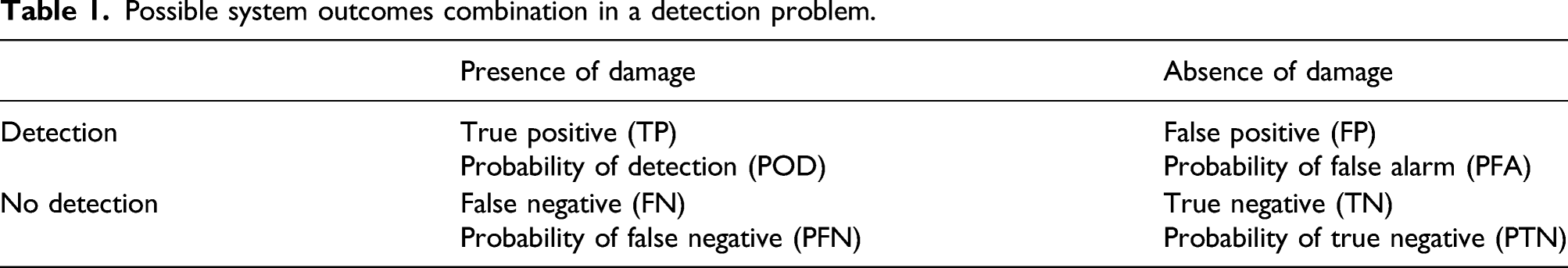
The POD is also often referred to as Positive Predicted Probability (PPP),
36
whereas the PFA is sometimes simply called Probability of False Positive (PFP).
22
In the same manner, the PTN can be named Negative Predicted Probability (NPP).
36
Summing the probability values of each columns in Table 1 always returns the value of one as a direct consequence of set theory.
22,36,37
Exploiting Bayesian conditional probability, it is possible to introduce the concepts of sensitivity and specificity. Calling P (AD) the probability for the structure to be to be healthy (absence of damage), P(PD) the probability for the structure to be not healthy (presence of damage), P (Det) the probability of the system to report a detection, P(NoDet) the probability of the system to do not report a detection, one has

The POD and PFA are useful in the design phase and to assess the reliability of the measuring system. On the other hand, under operational conditions it can be useful to refer to the other two probabilities: the Positive and Negative Predictive Values (PPV) and (NPV).
22
The engineer can use the PPV and the NPV to determine the conditional probability that a certain damage is present given that it was detected, which is crucial to take the right choice in terms of maintenance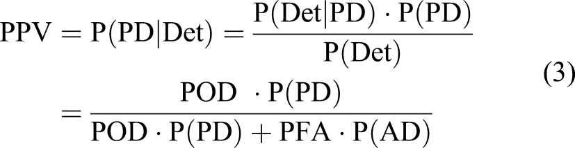
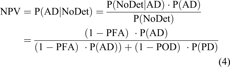
The comparison of equations (1) and (2) with equations (3) and (4) shows that while POD and PFA depends only on the inspection methodology, the PPV, and the NPV depend also on the prevalence. The prevalence is the likelihood of structural damage being present. In a low-prevalence scenario, the PPV can be relatively low even if the POD is high. 22,38
General considerations on probability of detection curves
In 1989, the studies of Berens 39 were included in the American Society of Metals (ASM) Handbook. Nowadays, the methodology to derive a POD is thoroughly described in the Appendix G of the MIL-HKBK-1823A. 16 The POD is a powerful tool that allows researchers to compare the performance of different monitoring techniques, 40 estimating the sensitivity and reliability of the inspection process. 41 Other definitions are available in the literature. 42–44
The United States Air Force (USAF), within the ASIP, employs POD curves to assess the reliability of various NDE methods. 45 In the aerospace industry, the POD curve can be exploited to perform risk analyses, to schedule inspections, to estimate the remaining useful life of a certain component, and to develop accept/reject criteria. 46 POD are also becoming attractive for other fields where they were traditionally less popular such as the nuclear industry. 47
In a POD study it is crucial to have enough data available. 48 A good practice would be to have at least a number of 40 data points. 16,49 Annis et al. investigated what should be the optimum sample size in a POD study and found that beyond 60 samples the improvement on the confidence bounds was less significant. 50 Further details can be found in the paper of Gandossi and Annis. 51 The minimum number of samples also depends on the POD model type. When logistic models are used, at least 60 samples are needed to avoid instabilities. 52 In Koh and Meeker, 53 it is presented a statistical procedure to plan a POD study introducing a dimensionless standardized flaw-size variable. However, since it is often unpractical to produce a statistically significant number of specimens, much effort has been devoted to develop strategies capable to reduce the required data.
â versus a method
The “â vs a” analysis is the most widely accepted method for the POD assessment in the NDE field. The symbol “â” is used to identify the measurement output whereas the “a” parameter denotes the damage size (i.e., crack length) responsible of generating that measurement signal. 16
From regression to probability of detection curve
Engineers are usually familiar with the Ordinary Least-Squares (OLS) linear regression. However, when dealing with censored data, the OLS would provide non-conservative results. In these situations other techniques such as the Maximum-Likelihood Estimation (MLE) method must be considered. In absence of censored data, the MLE method coincides exactly with the OLS regression analysis.
54
In both cases, the consistency of the models holds if six conditions are verified
52,55
. 1. The model must reflect the data. 2. It is required to have a continuous and observable response. 3. The linearity of the parameters must be satisfied. 4. The variance must be homoscedastic (uniform variance) about the regression line. 5. The observations must be uncorrelated (with respect time and/or space). 6. The errors must follow a normal distribution.
In the regression analysis, it is crucial to identify the right â vs a plot. Four possible combinations can be used: (i) â vs a, (ii) â vs log(a), (iii) log(â) vs a, and (iv) log(â) vs log(a). 56
A good practice would be to plot all the four possible graphs and choose the one with the best fit.
52
Considering the â vs a case (the same procedure can be extended to the remaining three cases), the two variables are related to each other with the following regression equation

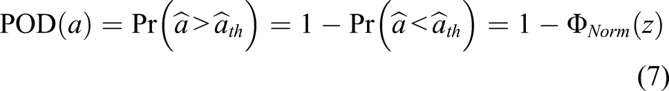
Here, 
Another way to express the POD is given by equation (9)
It is possible to identify two points of interest:
Choosing the right threshold
Every POD depends on the detection threshold. Arbitrarily lowering 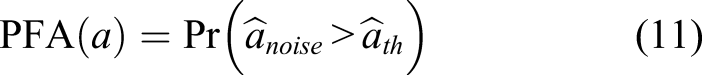
One could use the so-called Receiver Operating Characteristics (ROC) graph,
58,59
as a tool to determine the best threshold.
Probability of detection curve bounds
Confidence intervals express the statistical uncertainty due to the fact that only a limited amount of data is available. 46 The computation of the POD lower bound can be divided into two steps. First, the confidence and the prediction intervals (the latter differs from the former because they also consider the variability of the observations about the predicted mean) are computed using the Wald method. Second, the so-called Delta Method is applied to transfer these confidence intervals to the POD curve. The Delta method can be regarded as a technique for estimating the moments of functions of random variable, 64 and is applied to compute confidence bounds of non-linear functions. 65 Details about the math behind the Wald and Delta methods can be found in the MIL-HDBK-1823A. 16
With the aid of synthetic data, Figures 2 and 3 show the result of the â vs a method, and the POD curve with its corresponding lower bound using the Delta Method.
POD curve and its lower 95% Wald confidence bound using the Delta method.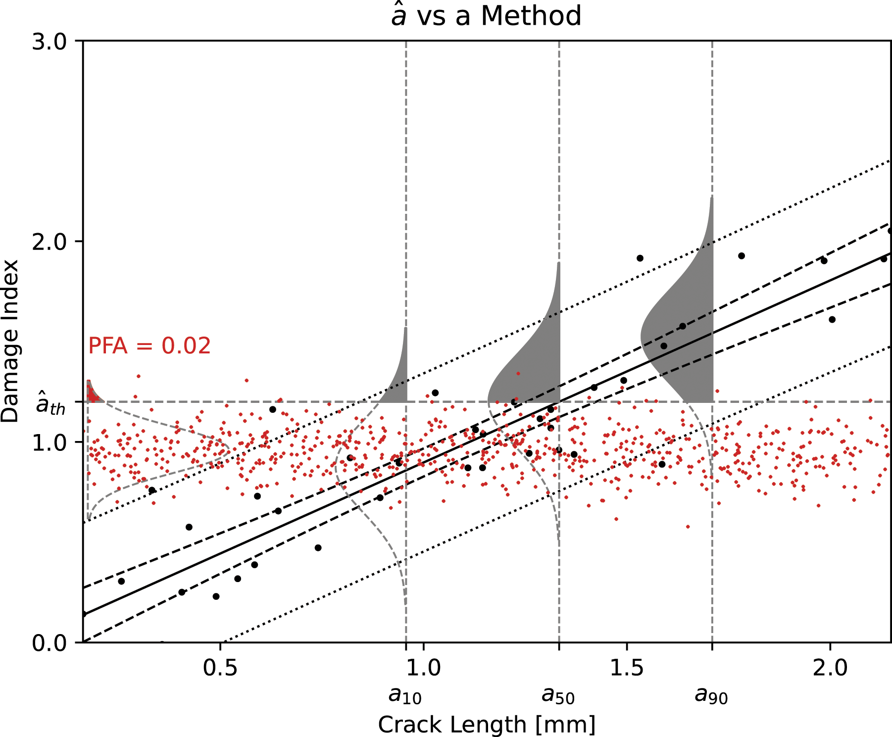
Binary (Hit/Miss) data
Historically, the first method to derive a POD was based on the ratio between the number of defects detected, n, usually cracks, and the total number of defects inspected in the structure, N. 16 Such approach implies an intrinsic tradeoff between the crack length and the POD resolution. Therefore, other methodologies were developed to overcome these statistical deficiencies. When dealing with hit/miss data, the system provides only a qualitative information specifically related to the presence or absence of damage in the structure. 36 The underling statistical models are based on Generalized Linear Models (GLS). The idea is to leverage continuous functions bounded in the interval [0,1], such as the logit, probit, cloglog, and loglog functions, 16 and use the maximum likelihood criterion to compute the model parameters. 66 The interested reader may refer to the following references to delve into POD for hit/miss data and the specific statistical methods to compute the corresponding lower confidence bounds. 16,67–74
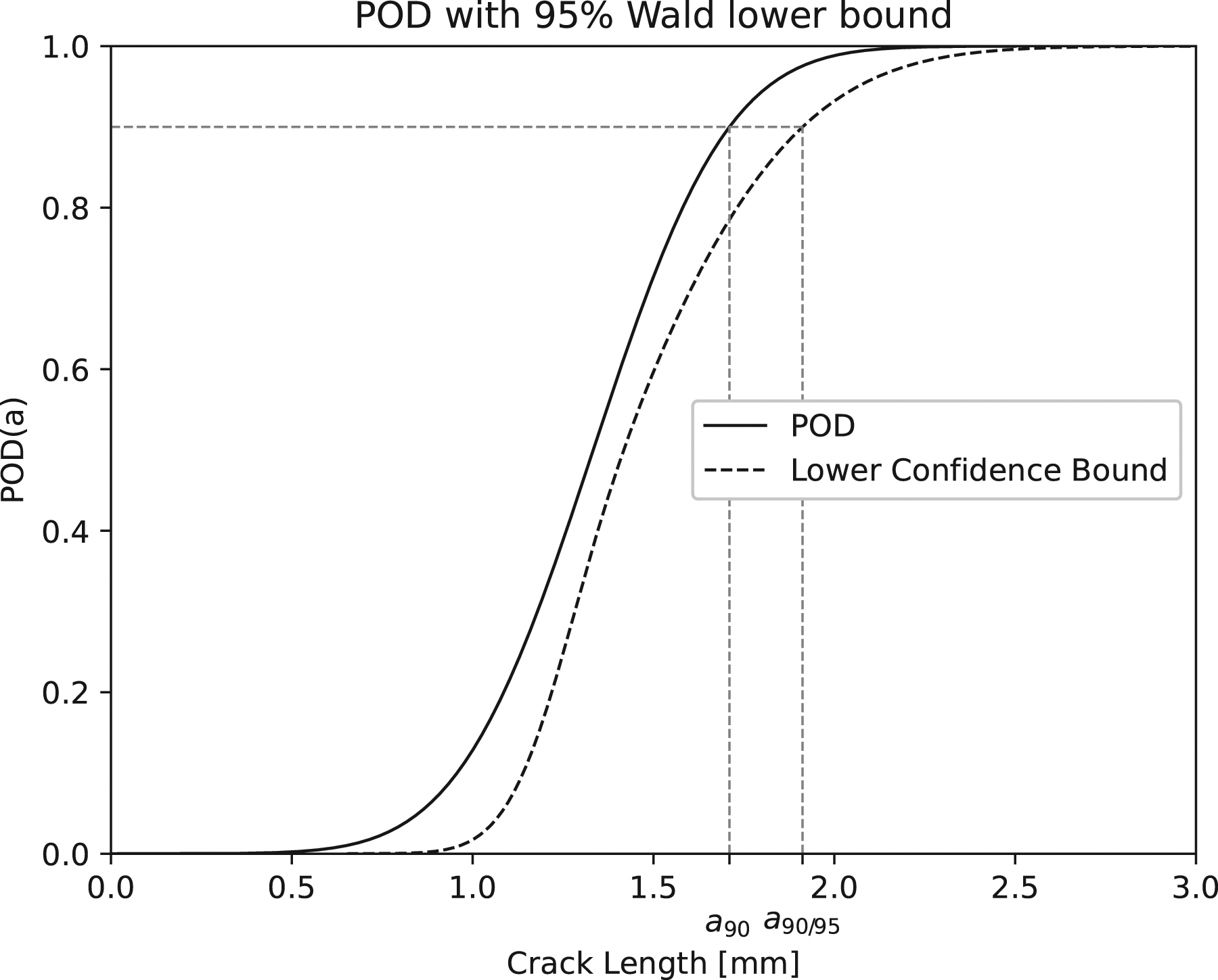
Variability sources in structural health monitoring
In a POD study, it is fundamental to capture all the possible variability sources. Incomplete variability considerations can lead to biased POD curve estimates. 46 Variability is linked to the intrinsic stochastic nature of the phenomenon under examination. 49 Therefore, increasing the amount of data would only shrink the confidence bounds but not the variability. Li et al. proposed the interesting idea of taking into account the inherent population variability using the 0.05 POD quantile estimate and then computed its lower confidence bound to consider also the uncertainty related to the model parameters. 75 Referring to a small quantile of the POD curve can be a more appropriate solution when the engineer is interested to consider the worst possible scenario. 76
In NDE one possible source of variability comes from the morphology of the cracks itself. 77,78 A portion of variability could be associated with the sensing device due to the manufacturing process of the instrument. Environmental conditions such as temperature and humidity may change the signal output of a certain measuring technique. 49 Finally, the human factor contribution in NDE systems is often considered the highest within all the variability sources. 79,80
Structural health monitoring systems inherit all the variability sources of NDE methods. The manufacturing process (sensors, interrogator, specimens, or test structures) 49 and damage morphology are examples of variability sources affecting both NDE and SHM systems. 78 The only exception is the variability associated with the human operator. The SHM system is usually capable of acquiring data automatically even in the areas where typical NDE inspection are unpractical due to complex geometries and accessibility limitations. 10 Nevertheless, stating that SHM systems are not exposed to human variability sources is not completely true. Indeed, the installation of the sensor network on the structure can be regarded as a human related variability source. 79
Moreover, additional considerations should be considered when performing a POD study in SHM systems. Sensor degradation is one of the main issues. Since the sensor are permanently installed in the structure, they are subjected to degradation over time due to aging and fatigue. Degradation may regard the sensor itself or its coupling with the structure such as the adhesive, welds, and dry couplings, depending on the technique. The system performance can also be affected by changes in the structure itself due to maintenance operations. It has been reported that sensor deterioration over a certain period of time has an impact on the POD curves. 54,81 Environmental and Operational Conditions (EOCs) like temperature, moisture, pressure, and chemical loading, can greatly affect the SHM system response, 82–84 while the same factors are expected to produce minor effects in a NDE system. Other sources of variability can be associated with the loading condition of the structure which can change over time (take-off, cruising, maneuvers, landing, etc.). The reciprocal position between the sensor and the damage is another specific aspect to consider in SHM. When considering POD curves of SHM systems, their relationship with the defect/damage location cannot be neglected because sensor location is a significant source of variability. 31,85 One could produce different PODs depending on the flaw location. 54 Moreover, there could be changes in the recorded signal response due to the on-board SHM device. 49 Mandache et al. suggests that in case of a self-powered sensor, where the recorded data is transmitted with a wireless connection to an on-board memory storage device, electromagnetic interference as well as other possible interference with the avionics are potential sources of variability. 86
Summarizing, while in NDE variability is mainly attributed to the human factor, in SHM it is equally important to consider the spatial (location uncertainty) 31,54,85,87 and temporal (environmental effects) 79,80,88 aspects of POD.
Variability Sources: NDE versus SHM.
N: Variability source not present; Y: Variability source present; YY: Dominant source of variability.
The consideration of variability sources in SHM regarding POD curves can be divided into the spatial aspects and the temporal aspects.
Spatial aspects of probability of detection
Optimal sensor placement using probability of detection
The spatial related variability of SHM system has been studied by several authors. 87,89,90 In many cases, the influence of the damage location on the detection performance translates in an Optimal Sensor Placement (OSP) problem. 87 Indeed, the presence of permanently installed sensors suggests that in SHM POD curves may serve not only as a tool to quantify the system performance but also as a tool for the design of the SHM system itself. OSP has been studied for several years and a wealth of literature has been produced. A recent review article written by Tan and Zhang summarizes the main advancement in OSP. 91 An important reference is the study of Flynn and Todd who were among the first to use the concepts of POD and PFA to develop a framework for OSP. 92 Similarly, Azarbayejani et al. demonstrated that OSP can be found maximizing the POD. 93 Markmiller and Chang used the POD as a design constraint for the OSP of an SHM system aiming to monitor the dynamic response of the structure caused by an impact event. 94 Mallardo et al. used POD curves to validate the performance of an artificial neural network whose aim was to detect the location of a certain impact in a composite plate and in a composite stiffened panel. The OSP was chosen such as the POD curves related to different sensor combinations were maximised. 95,96 Yan et al. used a model-assisted POD approach to validate the performance of different sensor configurations. 97 Chen et al. leveraged POD curves to determine the optimum Lamb wave driving frequency to detect fatigue crack growth in a metallic specimen. 98 Grooteman used POD as an objective function to obtain the OSP for optical fibers applied to a stiffened composite panel. 99 Tabjula et al. used outlier analysis to minimize the number of sensing points in a Guided Lamb Wave (GLW) study and POD were employed to quantify the system performance. 100
Specimens versus test structures
In NDE, a POD study is carried out testing several specimens. Similarly, in SHM one should employ a certain number of identical structures, which are the equivalent of the specimens in the NDE study. However, this makes an already expensive procedure even more difficult to apply. Identical structures in SHM requires identical sensing systems. Even though this is possible theoretically, Müller et al. showed that this is not feasible in practice. 79 This is the consequence of the amount of variability involved in the manufacturing process and sensors installation. Therefore, the POD curve will apply only for that specific structure and that specific sensing network configuration which was utilized to perform the POD study itself. For these reasons, the procedure becomes tremendously costly and time-consuming. Liu and Chang, in a US patent assigned to Acellent Technologies, propose to mimic the damage by bonding stiff metal or damping patches in the structure to create a POD database for a large structure. 101 However, the authors also stated that using real damages to produce these POD curves may lead to more accurate results. The introduction of real damages implies that the damaged structure might not be reusable, which increases the time and cost.
Decision threshold for structural health monitoring systems
Sometimes the damaged data may not be available or if available it might not be statistically relevant. In such cases, the threshold can be chosen by exploiting algorithms developed for unsupervised learning problems. 11 A multitude of methods are available in the literature within the field of novelty detection. Some methodologies require that the feature vector is normally distributed, such as outlier analysis. 102 On the other hand, other approaches such as extreme value statistics 103 can be used without the normal assumption to determine the best threshold value. A prominent reference is the review of Markou and Singh, which summarized the main statistical 104 and neural network based 105 approaches. Due to these additional challenges in determining the proper threshold, Cobb et al. suggests to use an hit/miss approach when dealing with SHM system. 106 Monaco et al. propose a methodology to evaluate the threshold level on a SHM GLW study based on the statistical analysis of noise. 36 In their study, the Kolmogorov–Smirnov test is used to reject the null hypothesis, being the non-Gaussian distribution of the experimental data. The same approach for the selection of the damage threshold has been used by Memmolo et al. in a study concerning the damage detection in a composite plate using a tomography technique based on GLW. 107 In Yue et al. 108 the detection of multiple barely visible impact damage (BVID) in large composite aircraft panels is achieved by outlier analysis using a reference pristine database gathered from simple coupons and mono-stringer panels under a wide range of temperature variation.
Temporal aspects of probability of detection
It is often stated that the major difference between NDE and SHM regarding POD development is that in the first case subsequent inspections are independent whereas in the second case they are correlated. Such statement is not entirely true. It would be more accurate to state that the degree of statistical independence between subsequent measurements is greater in NDE than in SHM. Statistical independence is a property that holds only for random events.
For example, Forsyth showed that the hypothesis of statistical independence is not completely true for repeated inspection related to simulated penetrants and eddy current testing. 41 This does not mean that one should jettison all the theory developed in MIL-HKBK-1823A, which assumes independent inspections. Even though several statistical independent degrees can be present, the hypothesis of independence might be true enough to lead to consistent results.
However, this hypothesis is not valid for SHM systems, where a continuous stream of data is expected to be recorded from the structure. The degree of correlation between measurements separated by a small-time interval cannot be ignored and must be properly handled. This intrinsic dependency of SHM measurements hinders the application of traditional statistical methods to produce POD curves, which is considered the most significant barrier preventing the widespread of the SHM technology. 34 In 2008 Shook et al. recognized this problem and developed a mathematical model to derive POD curves in the presence of repeated dependent data. 109 Discarding specific chunks of information might restore data independence but at the expense of compromising the effectiveness of the SHM methodology itself . 57 For this reason, several studies have been conducted to determine whether it is feasible to generalize the assessment methodology of the POD metric to SHM systems. 49
In the following section Sequential Data Analysis is introduced, showing how it can allow to deal with slowly evolving spurious signal changes due to EOCs, defect morphology, sensors drift and other kind of variability sources.
Sequential data analysis
As reported in Table 2, EOCs are predominant sources of variability in SHM. They can affect the detection performance of the system and their effect must be considered. In NDE it is possible to make measurements for a certain damage at varying EOCs. However, it is not possible to do the same in SHM. The output of the SHM detection system depends on the whole history of the EOCs. Moreover, this is coupled with the damage evolution, which leads to the need of studying a tremendous number of structures.
For instance, in ultrasonics SHM studies temperature has been reported to be the predominant effect in EOCs. 84,110–112 There are two main methodologies for temperature compensation: the Optimal Baseline Selection (OBS) and the Baseline Signal Stretch (BSS). A good description of the OBS method can be found in the paper of Lu and Michaels 113 whereas the BSS methodology is applied in several references such as Croxford et al., 114 Michaels, 115 Clarke et al., 112 Harley and Moura. 116 Recently, data-driven methods have been developed for effective temperature compensation of large temperature variation up to 70°C, 117 and for anisotropic materials. 118
Liu et al. proposed a hybrid approach to tackle the problem of slowly evolving spurious signal changes due to EOCs. 88 The authors evaluated the signal response of a pipe monitoring system under varying EOCs for the undamaged structure. Then, the damage effect was synthetically superimposed to the undamaged signal. A BSS algorithm was used for temperature compensation, and the baseline subtraction, Singular Value Decomposition (SVD) and Independent Component Analysis (ICA) damage feature extraction methods were compared. The ICA approach proved to the in general the most efficient to produce reliable ROC curves.
In a recent article, Mariani and Cawley summarize other temperature compensation techniques developed in the last decade. 119 Among them, the location-specific temperature compensation (LSTC) showed promising results for torsional guided wave signals in pipe monitoring, 120,121 resulting in a patent. 122 The same authors proposed a change detection algorithm based on the Generalized Likelihood Ratio (GLR) 123 applied to data obtained through the LSTC or the OBS methods. Their method proved to be sensitive to departures from the pristine state of the structure. However, the methodology only applies if the no sensor drift is present, which is one of the underlining assumptions of the change detection scheme. As a matter of fact, sensor aging and degradation remain an open challenge in the SHM field. Mariani et al. proposed a new methodology to address sensor drift on a thick copper block specimen. 124 They exploited the back wall echo ratio to reduce influence of PZT sensors drift. Another recent article of Mariani et al. leveraged causal dilated convolutional neural networks to both compensate EOCs and sensor drift. 125 Their algorithm, which is an adaptation of WaveNet (a deep neural network for audio waveforms), 126 outperformed the OBS and BSS approaches.
Probability of detection for structural health monitoring
In this section, three POD methods developed for SHM are presented, the Length at Detection (LaD) method, the Linear Mixed-effect Model (LMM) and the Random Effects Model (REM). These methods do not aim to address time dependent data in the way that a sequential analysis does. However, they provide different frameworks to handle the statistical dependence of the measurements being collected.
The length at detection method
The LaD model solves the dependency of sensor data, which is characteristic of SHM systems, by taking the measurement when the crack/damage is detected the first time. Therefore, there are not repeated measures because only the first crack detection is considered.
49
Roach et al. in 2007,
127
and Roach in 2009,
128
studied the reliability of Comparative Vacuum Monitoring (CVM) in aluminum and steel specimens using the LaD method. Sbarufatti et al. in 2016
129
and Sbarufatti and Giglio in 2017
130
applied the LaD methodology for fatigue crack monitoring on the tail boom stringers and fuselage panels of a helicopter using Fiber Bragg Grating (FBG) sensors within a model assisted framework. The crack size recorded in each test corresponds to the one for which a clear and stable detection signal is produced. Therefore, it all boils down to the task of characterizing the probability distribution of the crack lengths at detection and its cumulative distribution function represent the corresponding POD curve.
131
Assuming that the crack population shows a Gaussian distribution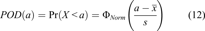
Similarly, if the crack population has a lognormal distribution, the crack length a in equation (12) is replaced by
The variables LaD method using 10 specimens (shown by different markers). Each specimen has 40 measurements.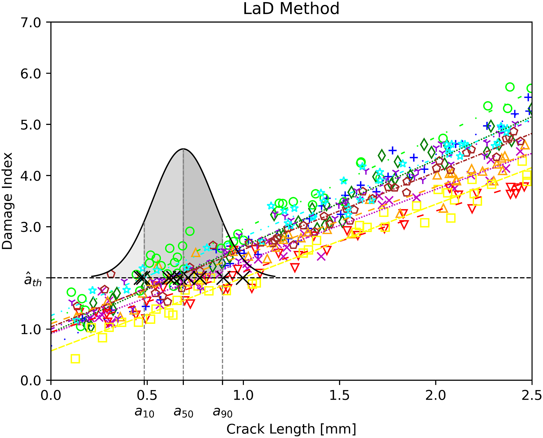
The confidence bound can be computed exploiting statistical methods relying on the non-central t distribution,
49,133
or applying the One-Sided Tolerance Interval (OSTI) approach. This methodology was firstly proposed by Roach in the detection of fatigue cracks using CVM. It provides an estimation of the upper bound containing a certain fraction of all measurements in the population with a given confidence level.
9
The percentage of all measurements and the confidence level are the main factors affecting the result. The former is usually taken equal to 90% whereas the standard for the degree of confidence is 95%. The OSTI approach can provide a reliable analysis with only eight flaws with respect the 51 required in a classic binary data POD.
134
Using the same symbols found in Roach,
128
the upper bound for the tolerance interval is given by
Linear mixed-effect model
Kabban et al. developed a statistical model in 2015 to produce POD curve for time-dependent data extending the classical â vs a methodology.
57
Since the observations are no longer uncorrelated, it is not possible to use OLS or MLE.
55
One possibility is to rely on generalized least square models (originally developed by Aitken in 1936
137
), which are capable to handle such time dependency .
57
The second possibility is to use a Linear Mixed-effect Model (LMM). This kind of approach extends classical linear models and are particularly suited for datasets where data are not truly independent. The LMM acronym comes from the fact that the “model” to be fitted is “linear,” and that there is the presence of a “mixed effect”: a random effect (this could be the intercept or the slope) and fixed one which generally describes the expected trend of the data. The synthetic data which were considered in the study of Kabban et al. suggested to apply a LMM with a random intercept.
57
Therefore, using the same terminology employed by the authors, there is a random intercept term for each experimental unit (EU), which is regarded as the basic primary experimental item used to collect data. Equation (14) explains how this approach translates in mathematical terms
The term
Random effects model
This model, sometimes referred to as Repeated Measures Random Effects Model (REM2),
138
tries to generalize the â vs a analysis described in MIL-HKBK-1823A for SHM systems.
49
Moreover, it takes a step forward with respect to the LMM developed by Kabban et al.,
57
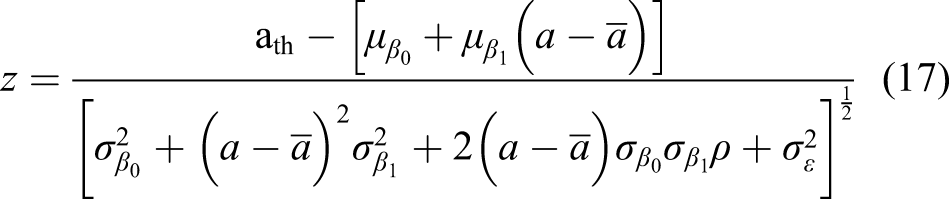
in the sense that it considers the possibility to have at the same time a random intercept and a random slope. Every crack-sensor combination will produce a series of data which can be fitted using a line with its own slope and intercept. Therefore, the method computes the joint distribution of these parameters
49

The subscript “i” denotes a certain crack-sensor combination, and “j” indicates a specific reading coming from that crack-sensor pair. Therefore, 
At the numerator REM method using 10 specimens, each one with 20 measurements. The red dots indicate noise measurements.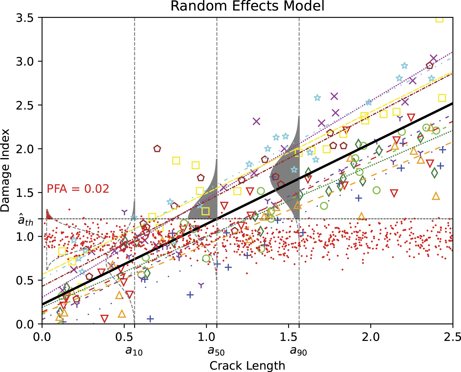
The computation of the corresponding lower bounds can be achieved with a MLE approach but Bayesian methods with weekly informative priors are also an option. The interested reader can delve into the work of Meeker et al. for further details about these procedures. 49
Comparison between length at detection and random effects model methods
In this section are discussed the main differences between the LaD and the REM methods. Since the REM method is a generalization of the LMM approach, the latter is not considered in this analysis.
Both LaD and REM model are valid statistical tools to evaluate POD curves for SHM applications. The LaD approach has been particularly used to evaluate the CVM performance in aerospace structures. Thanks to the Federal Aviation Administration (FAA) research program in SHM started in 2011, recently in the U.S. the use of this approach started to be accepted from the major original equipment manufacturer (OEM) and airline operators such as Boeing and Delta.
139
Despite the LaD offers a relatively simple approach, it discards some information, thus it does not exploit the full potential of the specific SHM application. It also requires an assumption about the crack length at detection distributions (not always easy to verify) and different distribution choices can lead to significantly different results. On the other hand, the REM uses the whole dataset, and this also implies the model to be more robust against departures from the model assumptions. More important, it can be compatible with a model-assisted approach, which makes it very attractive for future applications. A study made by O'Connor tried to quantify the difference between these two statistical methods.
140
From a qualitative point of view, it is pointed out again the fact that it is difficult to justify the use of a certain distribution (normal or lognormal) in the LaD method. Nevertheless, when few observations are available (less than 10) the LaD method seems to be more appropriate since it may be not possible to fit a 5 parameter REM. Therefore, since the LaD it is also lighter from a computational point of view it might be preferable in certain engineering applications. In reference
140
the two methods are also compared quantitatively using as reference the a90 values computed for different datasets. The LaD seemed to overestimate the a90 when the normal distribution approximation of the crossing lengths was not appropriate. However, this results in a conservative prediction, which can be acceptable from an engineering point of view. The two methods showed comparable results except for situations where the
Previous SHM studies tended to neglect data dependency but now the literature highlights that this is not the right way to proceed. Despite these statistical methods are relatively new in the SHM field, there are already several case studies where they are leveraged. Recently Kessler et al. made use of both LaD and REM approaches to develop POD curves. 138 The authors used a 4-point bend test to obtain a crack growth starting from an Electrical Discharge Machined (EDM) notch on Aluminum bars. They monitored the crack evolution with a carbon nanotube (CNT) sensor, which have a great potential for aerospace applications. 141 A recent study, using the methodology proposed by Meeker, 49 made use of a Bayesian approach to derive POD curves for different case studies. 142 Typically, in the majority of the SHM systems based on ultrasound techniques, the relationship between the damage index and the damage size is not linear, which goes against the assumption made by Meeker. 49 However, linearity can be restored applying a logit transformation to the damage index.
Multivariate-probability of detection
One single parameter may be not sufficient to describe the defect characteristics satisfactorily. In evaluating the corrosion present in aircraft structures, Bode et al. derived POD curves as a function of both defect size and percent corrosion. 143 Lee et al. created a M-POD surface using a multivariate log-logistic regression model based on hit/miss detection, where both the defect length and depth are considered as parameters in a ECT application. 144 In a similar ECT study, Hoppe developed a M-POD as a function of crack length, l, and depth, d, but this time extending the classical â vs a method. 145 In 2012 Aldrin et al., along the lines of the previous work of Hoppe, 145 found that including the crack depth in addition to the crack length was reducing the model uncertainty of about 20%. 146 The same authors leveraged a physic-based model (VIC-3D©) to consider several parameters and thus to reduce the variability and the required number of samples. Another case study regarding the ECT of fastener sites for fatigue cracks, 147 revealed that the calibrated physic-based model, which considered multiple parameters rather than the simple crack length, performed better with respect the classic â vs a method. 148 Pavlović et al. 149 developed a M-POD for an ultrasonic inspection of a cast iron component. With this approach it was possible to compute several POD curves as a function of the desired variable holding the other parameter values. Yusa and Knopp pointed out that the M-POD in Pavlović et al. 149 was based on 12 coefficients which were not easy to compute, and that it is unlikely to have a uniform variance. 150 Therefore, they proposed a multi-parameter approach where even the variance is a function of the parameters instead of being constant. Alternatively, in Gao et al. can be found a linear mixed effect model describing the response of a vibrotermography test as a function of the vibration amplitude, pulse length, trigger force and crack length. 151
Only recently, M-POD related to SHM systems with permanently mounted sensors have been studied. M-POD models are particularly attractive for SHM applications systems because they provide frameworks to include the extra variability sources typical of SHM systems. To bring this approach into the SHM world, the aid of numerical simulations seems to be unavoidable. For SHM, M-POD often requires the use of a model assisted approach.
Model-assisted probability of detection
Model-Assisted Probability of Detection (MAPOD) curves have their roots in NDE but at the same time provide a framework suitable for SHM studies. 49 An extensive review of MAPOD studies can be found in the Pacific Northwest report written by Meyer et al. in 2014. 152 This research field was pioneered by Thompson, who guided from 2003 to 2010 the Model-Assisted Probability of Detection (MAPOD) Working Group at Iowa State University. 153 One objective of a MAPOD study is to reduce the amount of experimental data, required to generate a reliable POD, gathering additional information through a physics based model. 154 There are two main MAPOD variants: the transfer function approach (XFN) and full model-assisted methodology (FMA). 46,154
The XFN exploits the relationship existing between the output signal of real flaws and synthetic produced flaws which are easier and less costly to realize. 155 Using the XFN approach, starting from an existing fully empirical POD curve for a certain technique, it is possible to transfer these results to another similar configuration. The underling transfer function may be computed exploiting a physic based model or by specific laboratory tests. 156
The FMA approach aims to predict the signal strength of a certain NDE/SHM technique as a function of several parameters and flaw properties, capturing all the variability sources, combining the information provided by physics-based models with empirical knowledge 156 such as experimental noise. 157 The first attempts were made on ultrasonic testing methods but the FMA concept is general and can be applied to other sensing techniques. 46
Thompson concluded that the XFN and the FMA approaches were just two sides of the same coin. 156 In 2008 a unified approach for MAPOD was proposed in the form of a protocol, 154 and later on the methodology was included in the MIL-HKBK-1823A. 16
Gianneo et al., taking the work of Pavlović et al. 149 as reference, leveraged MAPOD in a study concerning GLW for SHM systems with lightweight material. 83,85 From the M-POD curve (called in the paper “master” POD) the authors derived several conventional POD curves as a function of single parameters like the flaw size, the angle with respect the PZT sensors and the Lamb wave mode (A0 or S0). On the other hand, the remaining parameters were treated as random variables. When numerical models are employed, their success in capturing all the variability sources strongly depends on the known unknowns. 158 Previous knowledge about the important variables is indeed important to obtain variability data sources from experiments and to integrate them into the numerical models using noise signals as an example. For instance, Memmolo et al. decided to use a MAPOD approach for a GLW based SHM technique. 159 The variability sources were considered by adding a random noise to the FEM model output and randomly choosing parameters that are related to the damage such as its morphology and its position in the structure. Tschoke et al. studied the feasibility of MAPOD to produce POD maps in an automotive component made of Carbon Fiber Reinforced Polymers (CFRP) obtaining promising results. 90 This can be considered a M-POD since the additional parameter of the damage location is considered. Similarly, Leung and Corcoran evaluated the POD spatial distribution and combined this information with the probability of defect location. 87
Metamodels
In general, the computational effort increases with the number of variability-related parameters considered in the M-POD. High dimensionality problems require many model evaluations that need to be run, which can be a prohibitive process. A possible solution to lessen the computational burden is to leverage metamodels. Metamodels, sometimes referred to as surrogate models, are basically a simplified model of the original physics based model. 160 For example, CIVA 161,162 is a software that allows to use metamodels for Model Assisted POD studies both in NDE and SHM applications. Moreover, they can be used for other purposes such as sensitivity analysis evaluating the Sobol indices or to derive nonparametric POD curves. 160,163
Miorelli et al. show that in the CIVA software metamodels can be derived using the Output Space Filling Criterion or the Support Vector Regression algorithm. This kind of solution is particularly important in MAPOD studies. Engineers are often making assumptions about the probability distributions of the parameters related to variability source. These assumptions are difficult to verify, and a huge number of simulations is required to explore all the possible parameter combinations. Relying on conventional physics-based models leads to unfeasible computational times for practical applications. Dominguez et al. developed an algorithm to generate beams of POD curves and derive confidence bounds. 164 They generated a database to develop a surrogate model. The process is computational expensive but if beams of POD must be produced, the procedure becomes soon convenient.
Bayesian methods
Bayesian statistics can be regarded as another useful tool to manage the high amount of requested data. 165 It provides a mathematical framework to take advantage of prior knowledge for inference and decision making. 166 In this case the prior regards the quantity and type of damages present in the structure. Prior belief can then be updated once new experimental evidence is available. One may be wondering why this approach that seems to fit so nicely into this problem has not been considered in the past. The answer is that it can be very time consuming from a computational point of view. Nevertheless, recent progresses in terms of high-speed computing, made possible the easy implementation of Markow Chain and Monte Carlo techniques. These algorithms, combined with the use of physic-based models, allow the derivation of the likelihood required in the famous Bayes’ formula. Even in the case of having a poor informative prior or not having it at all, this approach can be applied simply considering a uniform distribution of the prior. In this way the posterior will not be affected by the prior belief and relies entirely on the likelihood. The likelihood could be derived experimentally but also exploiting physics-based models information. 167 Despite Bayesian statistics has already been leveraged in the field of NDE to develop POD curves, 168–171 to the best of the authors knowledge its use in SHM reliability studies is limited. The Bayesian approach has the benefit of exploit the full response of the measuring system in contrast with conventional methods where the only information that is considered is whether or not a certain threshold is exceeded. 172 Therefore, this is a promising field of research for SHM that should be further investigated.
Fusion of probability of detection curves
An SHM system is made of several sensor-damage combinations. Moreover, different types of sensors may coexist in the same structure with the aim of providing complementary information. Therefore, for the same structure several POD curves are expected to be produced, each one related to a certain measuring technique. Ameyaw et al. applied the concept of POD curves to vibration based fault detection and isolation (FDI). 56,173,174 It was found that, depending on the sensor type, position and damage location, different POD curves are generated. Therefore, it was considered reasonable to develop a strategy to combine different POD curves related to different sensors. In this way all the available information is utilized, and the system reliability is expected to improve. Ameyaw et al. proposed a methodology in which, rather than fusing all the POD curves into a single POD curves, several belief values are computed using the Bayesian Combination Rule (BCR). 56,173,174 In this approach, all the possible sensor combinations are considered. For example, a certain damage could be detected (i.e., signal higher than the threshold value) only by certain sensors (each sensor with its own POD curve). By applying the BCR for each possible detection/missed detection combination, it is possible to derive a corresponding number of belief curve as a function of the damage size.
Nevertheless, it is often not desirable to fuse the curves as it dilutes the available information. It would be more appropriate to apply sensor fusion at lower level and derive a single POD curve using a single damage index combining features extracted from different sensors. Several fusion algorithms exist in the literature 11,175–177 and therefore it is reasonable to think that more than one strategy may be applied.
Localization and sizing metrics
Probability of localization
The second phase of a SHM system aims to localize damage and this section analyses the main progresses made to quantify the localization performance. Localization is only related to unknown damage location (UDL) SHM systems. Known damage location (KDL) SHM systems, sometimes also referred as hot-spot monitoring, do not require any localization as the damage position known. However, must be clarified that hot-spot monitoring is not NDE. Even if they share the fact that damage location is known, they cannot be treated using the conventional NDE methods because all the considerations regarding data correlation discussed in the previous sections. Nevertheless, damage localization remains an essential component of the SHM paradigm because (1) it is not always possible to identify hot spots where damage is likely to occur in the structure, and (2) unexpected events such as impacts, or unknown failure mechanism are always possible. Moreover, SHM systems can produce information beyond mere damage existence. Therefore, additional metrics are required to reach adequate reliability standards.
Aldrin et al. in their study claim that such metric should consist of an error with its corresponding uncertainty related confidence bounds.
23
They gave an example with a potential candidate, the so-called Normalized Localization Accuracy (NLA)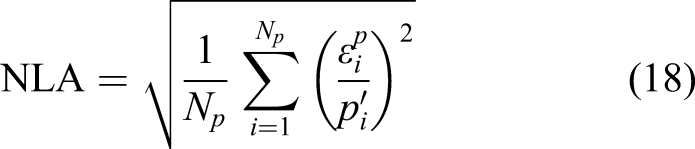
The terms in equation (18) are the number of location estimates, 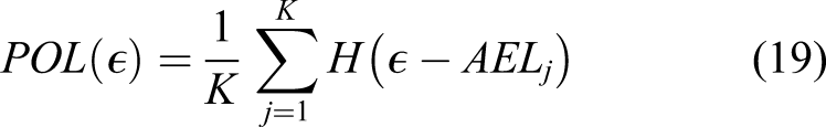
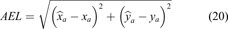
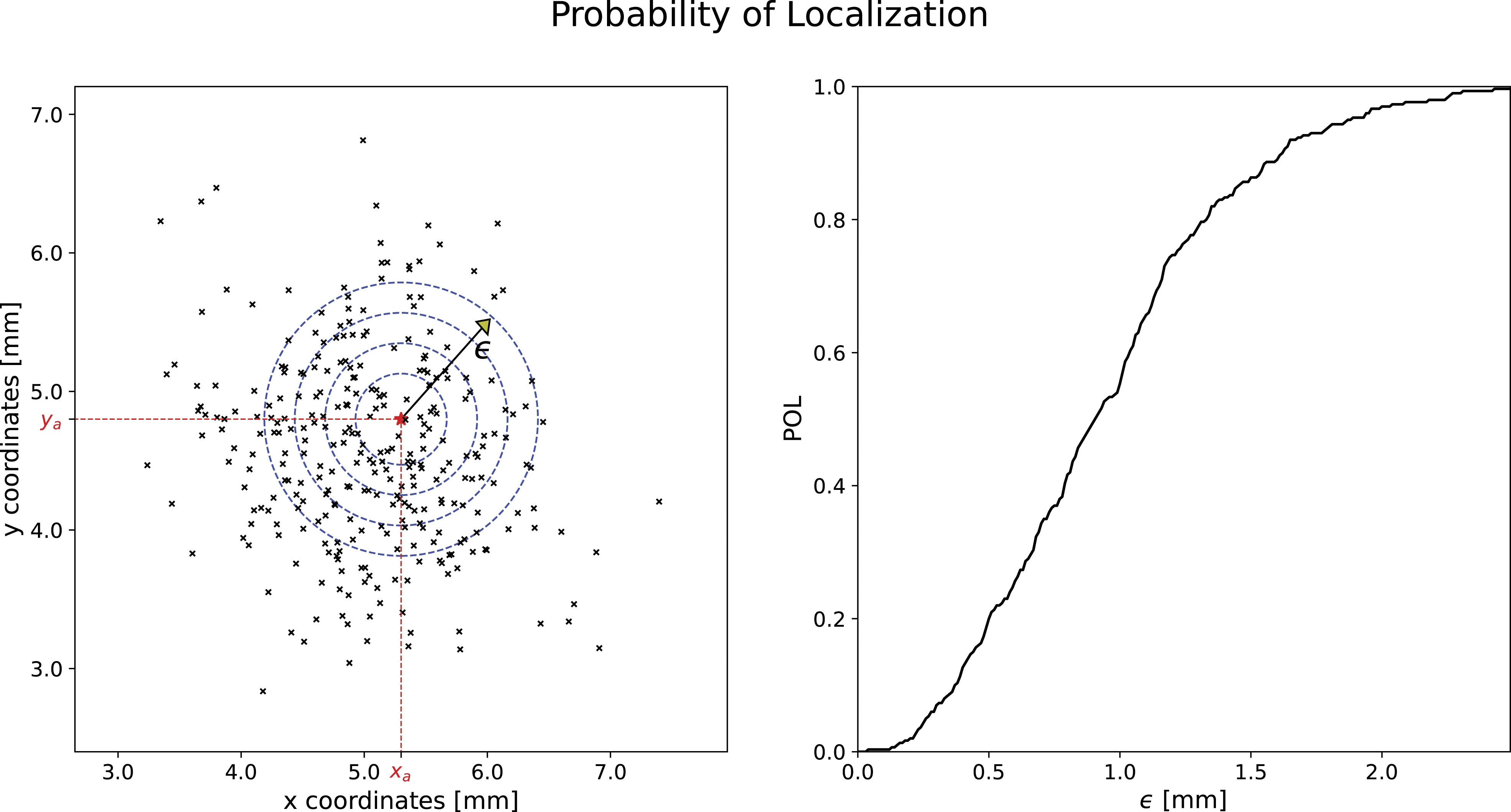
The symbol H represents the Heaviside-step function. In this way, are counted only the cases where POL computed according to the methodology of Moriot et al.
181
The same authors introduced the concept of Model-Assisted Probability of Localization (MAPOL) as a tool to generate synthetic data and build POL curves. Despite this methodology represents a step forward to derive a reliable localization metric in analogy with common POD curves, it has the drawback of having confidence bounds without any meaning because the POL is not the result of any regression task. This lack of uncertainty evaluation capability makes this approach not appropriate for many applications where decisions are made according to an acceptable risk.
Yue and Aliabadi studied a hierarchical approach for determining the reliability of SHM systems using guided waves.
182
The third level of such methodology regards damage localization and its performance metrics. They proposed to use the concepts of trueness and precision
183,184
to quantify the accuracy of the damage location estimations. The trueness, typically associated with a systematic error, is defined similarly to the AEL Location accuracy estimation with trueness and precision according to Yue and Aliabadi.
182
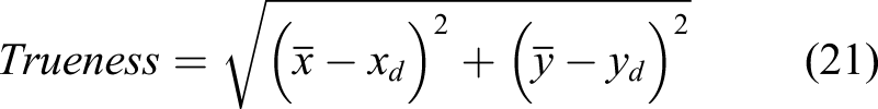
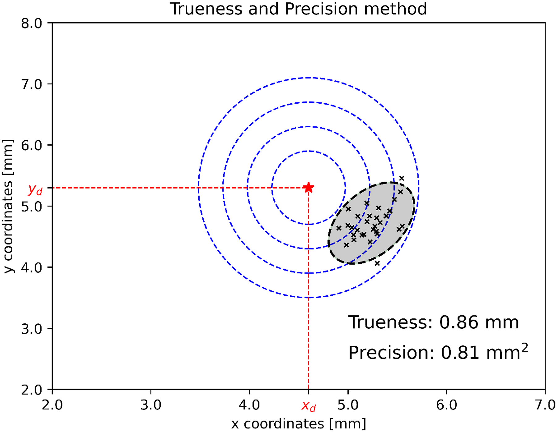
The same authors developed a probabilistic framework based on the Bayes’ law to quantify the probability of determining in the correct manner the damage location inside a selected area.
182
Leung and Corcoran developed the interesting concept of Probability of Damage Location (PDL) maps
87
that can be mathematically expressed as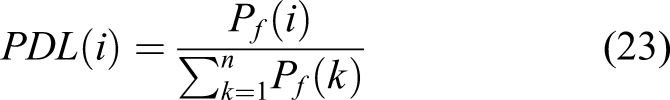
There has been an increasing interest in the development of many different localization metrics. In the future much effort should be posed in defining a common methodology to lay the foundations for an accepted standard.
Probability of sizing
In the third phase of a SHM system, the main objective is to characterize the damage being previously detected and localized. Although the previous two phases do not leave room for any misinterpretation, damage characterization or identification can be confusing. Depending on the specific application there could be the necessity to quantify the damage size, classify the different damage shapes or different damage types. Taking composite material as an example, being able to classify matrix cracking, delamination, fiber breakage, and fiber pull-out is as important as determining the actual damage size.
The Probability of Sizing (POS) could be regarded as the probability of correct sizing a damage or a defect. In other words it describes the accuracy of estimating the size of a defect. 185 Attempts to evaluate the sizing accuracy of a certain measurement technique have already been made in the past. 186 For example, in Automated Ultrasonic Testing (AUT) researchers evaluate the sizing performance using the so-called safety Limit against Under Sizing (LUS). The LUS metric, also known as 95% LUS, can be thought as the lower 95% uncertainty bound of the linear regression model where the true size of a certain flaw (usually evaluated with destructive testing) is plotted against the value given by AUT. 187,188
Annis et al. recommend being particularly cautious in the use of the LUS metric. Indeed, the assumptions upon the LUS is based, such as the linearity in the response and the homoscedasticity of the variance are not necessarily true. 55 More in general some authors, in analogy with the “â vs a” analysis, perform a regression task between the measured versus actual damage sizes. 189–192 For example, Lee et al. quantify the reliability of sizing results for axial outside diameter stress corrosion cracks, spotted near the top of tube sheet in steam generator tubes. 144 They compute the coefficient of determination r 2 related to the linear regression analysis between the true size, estimated by destructive examination, and the measured size, obtained by eddy current test (ECT). The r 2 score is then used as a reference to estimate the sizing performance of the ECT technique. Ginzel et al. retrieved the equations originally developed by Ermolov in 1972 193 in order to predict the size of flaws given by ultrasonic methods. 194 The authors pointed out that the sizing accuracy depends on many parameters, depending on the measuring technique, the material, the structure layout, the defect orientation, etc. Nath et al. proposed to assess the reliability of the Time-of-Flight Diffraction (TOFD) inspection method in terms of POD and POS curves. 189,190,195 Specifically, POS curves are developed similarly to POD curves using the â vs a method but replacing the signal response with the measured defect size in the â value. Then, the decision threshold was set arbitrarily to a certain value or equal to the maximum difference between the measured flaw size â (the depth in that specific case), and the actual flaw size. Despite the fact Nath et al. claimed to have developed POS curves, the way such curves were built is not in compliance with the definition of POS. 185 Indeed, the curves built in such way represent the probability that the estimated defect size is greater than a certain size and not the probability of correctly sizing the defect itself. Alternatively, performing several inspections on a series of representative damages, it is possible to develop a probability density function relative to the damage severity which is used to obtain an upper bound on the damage size. 196,197
Aldrin et al. claim that a sizing metric should consist of an error with its corresponding uncertainty related confidence bounds. 23 They gave an example with a potential candidate, the so-called Normalized Quantification Accuracy (NQA), which is a metric analogous to the NLA (see Probability of localization) but related to sizing. In 2014, in the attempt of better formalizing the current sizing and localization metrics, was introduced the Characterization Error (CE), ê, which is the difference between the estimated damage characteristic (location, size, depth, width, etc.), â, and the actual damage state, a. 45 This new metric it is likely to be developed upon the mathematical framework provided in the MIL-HKBK-1823A, but is expected to be more complicated than traditional POD studies, requiring both engineering and statistical expertise to be applied. Poor characterization results could be attributed to a low signal to noise ratio, measurements close to the saturation level, ill-posed inversion problems, failure mechanisms which are independent with respect to the defect size. 198
Despite defect characterization, and hence sizing, represents the third fundamental level of SHM, 32 to the best of the authors knowledge there are not specific case studies which have attempted to develop such metric for SHM systems.
Discussion and perspectives
In this article, the evolution of POD and the development of localization and sizing metrics has been described. This section summarizes the most relevant studies in the field (as shown in Table A1 in Appendix) and discusses future perspectives in SHM reliability metrics.
The first observation arising from the “Field” column of Table A1 is the progressive shifting from NDE toward SHM studies, confirming the growth of the SHM field.
The “Metric” column shows that most of the studies are related to POD curves and only few of them focus on localization and sizing. There is still a high heterogeneity in metrics for localization and sizing and there are not unique well-established definitions with an accepted standard. Moreover, the relationship between these metrics should be analyzed because SHM systems may have a hierarchical approach where damage detection, locating and sizing are performed in a subsequent order. The final decision regarding the reliability of a SHM system could be based considering all these metrics.
Sequential data analysis proved to be efficient to address the important challenge of dealing with serially correlated time series data in SHM due to varying EOCs, defect morphology and sensor drift.
Statistical methodologies such as the LaD, LMM, and REM are becoming the new standards in the field. Although the LaD is a relatively simple approach, the LMM and the REM are more complex and require a sound understanding of advanced statistical tools.
The use of M-POD in SHM requires the aid of numerical models to compute POD curves as a function of several parameters. MAPOD are therefore becoming fundamental tools for the derivation of M-POD. The biggest challenge is being capable of capturing all the variability sources of the system. As the number of parameters considered increases, the computational time rises tremendously due to the curse of dimensionality. Metamodels are good candidates to solve this challenge since they can reduce the simulation time of many orders of magnitudes, allowing the production of beams of POD curves.
When multiple sensing systems are employed, POD fusion methodologies can be used. This topic is still in its infancy and is not clear yet if it makes sense or not to fuse different POD curves since it may dilute the available information. However, fusing different sensors information at a lower level could produce more effective damage indices, thus improving POD curves.
There are no methodologies available in the literature to handle hit/miss data in SHM because all the POD for SHM stem from the â vs a case. When hit/miss data are present in SHM they are erroneously treated with conventional methodologies used in NDE. Therefore, there is the need to further investigate this topic.
The “Sensing” column showcases all the sensing techniques used in reliability assessment studies. A multitude of measurement techniques have been used but at the same time others are unexpectedly rare. For instance, despite acoustic emissions 199 and distributed optical fiber sensors 200 showed to be promising technologies in the field of SHM, reliability studies concerning these techniques in terms of POD curves are still limited to few studies.
The lack of specific reliability metrics is one of the major impediments for the validation and certification of SHM system. The “Objective” column highlights that there are many studies trying to assess the reliability of a specific system, but only few studies focus on the development of new reliability metrics. This discrepancy suggests that more effort should be posed in the derivation of common standard procedures to evaluate the performance of SHM systems in terms of detection, localization and sizing.
Even though a SHM study should be conducted with a real representative structure rather than simple specimens (as is typically done in NDE), this is not entirely reflected in the “Material and Structure” column of Table A1. Despite few exceptions, 88,119 most of the analyzed literature uses simplified structure components or even specimens to develop POD curves.
The situation highlights two requirements for a POD study in SHM that go in opposite directions: the need of reproducing a test structure as similar as possible to reality which is capable to capture all the variability sources, and the need of many such structures to obtain a statistically relevant study. The number of SHM studies leveraging numerical models for the development of POD curves has an increasing trend, as shown in the “Numerical Analysis” column. However, it is often difficult to substitute completely experimental data since the model could not be able to represent accurately the real structure or to capture or the variability source. A hybrid approach where experiments and numerical simulations are both exploited seems to be the most promising strategy. 88 Bayesian statistics could be used to integrate these two kinds of information. To the best of the authors knowledge this has only been done for NDE POD studies and should be object of further investigation also for SHM systems where the issue of having a large amount of data is even more exacerbated.
The column title “Damage and its Estimation” of Table A1 emphasizes that POD curves are plotted as a function of the estimated damage size rather than the true damage size. This point has never been addressed because it was implicitly assumed that the measurement technique used to address the true damage size was much more accurate than the value provided by the SHM system. Even if this assumption can hold, in many cases it does not or it is simply impossible to prove it. Therefore, this topic should be further investigated to implement the crack length estimation uncertainty in the current SHM methods to derive POD curves.
The concluding remarks of this review article are summarized below: • The SHM field is increasing faster than the development of its reliability metrics. There is the need of further research to develop statistical methods capable of quantifying the performance of SHM systems. • Is not possible to use conventional NDE POD curves in SHM. • POD curves are usually developed assuming zero uncertainty in the damage size which is not always acceptable. • Sequential data analysis can be used to study SHM systems under varying EOCs and to address problems where sensor drift is present. It is a promising research field which deserves further research. • Statistical models to generate POD in presence of dependent data are available (LaD and REM) but few studies use them to produce POD curves. • Multiple parameters can be considered using M-POD. In M-POD studies the use of MAPOD is fundamental. The curse of dimensionality can be addressed using metamodels. • Fusing data from several sensor sources may improve the POD and ROC curves. • Capturing all the variability sources is the key to obtain reliable numerical models and meaningful experiments. • Bayesian methods can be used to combine experimental and numerical data in POD studies for SHM. Recent studies showed that this approach is promising. • Despite recent studies developed metrics for localization and sizing, there is not a common well-accepted standard as for POD curves. Research is needed to produce a protocol capable of unifying these scattered efforts, using statistical tools capable to produce confidence intervals.
Footnotes
Declaration of conflicting interests
The author(s) declared no potential conflicts of interest with respect to the research, authorship, and/or publication of this article.
Funding
The author(s) received no financial support for the research, authorship, and/or publication of this article.