Sage Journals: Discover world-class research

Abstract

The value of using permanently installed monitoring systems for managing the life of an engineering asset is determined by the confidence in its damage detection capabilities. A framework is proposed that integrates detection data from permanently installed monitoring systems with probabilistic structural integrity assessments. Probability of detection (POD) curves are used in combination with particle filtering methods to recursively update a distribution of postulated defect size given a series of negative results (i.e. no defects detected). The negative monitoring results continuously filter out possible cases of severe damage, which in turn updates the estimated probability of failure. An implementation of the particle filtering method that takes into account the effect of systematic uncertainty in the detection capabilities of a monitoring system is also proposed, addressing the problem of whether negative measurements are simply a consequence of defects occurring outside the sensors field of view. A simulated example of fatigue crack growth is used to demonstrate the proposed framework. The results demonstrate that permanently installed sensors with low susceptibility to systematic effects may be used to maintain confidence in fitness-for-service while relying on fewer inspections. The framework provides a method for using permanently installed sensors to achieve continuous assessments of fitness-for-service for improved integrity management.

Introduction

The life of an engineering component is conventionally managed by a combination of structural integrity assessments and periodic manual non-destructive evaluation (NDE) inspections as shown in Figure 1. At regular intervals during service, an NDE inspection is carried out to ensure no defects exceeding a certain critical size are present (a negative inspection result). Following a negative inspection result (i.e. no defects detected), the fitness-for-service (FFS) is evaluated by postulating the existence of ‘the largest defect that might be missed’ and forecasting its growth. The remaining life of the component is then calculated based on the size of the postulated defect and the projected time to a limiting critical integrity state. This subsequently provides assurance on the integrity of the component and confidence in its FFS for a calculable period.

Figure 1.

Illustration of the typical life-cycle management of a component and the addition of monitoring data (shown in red).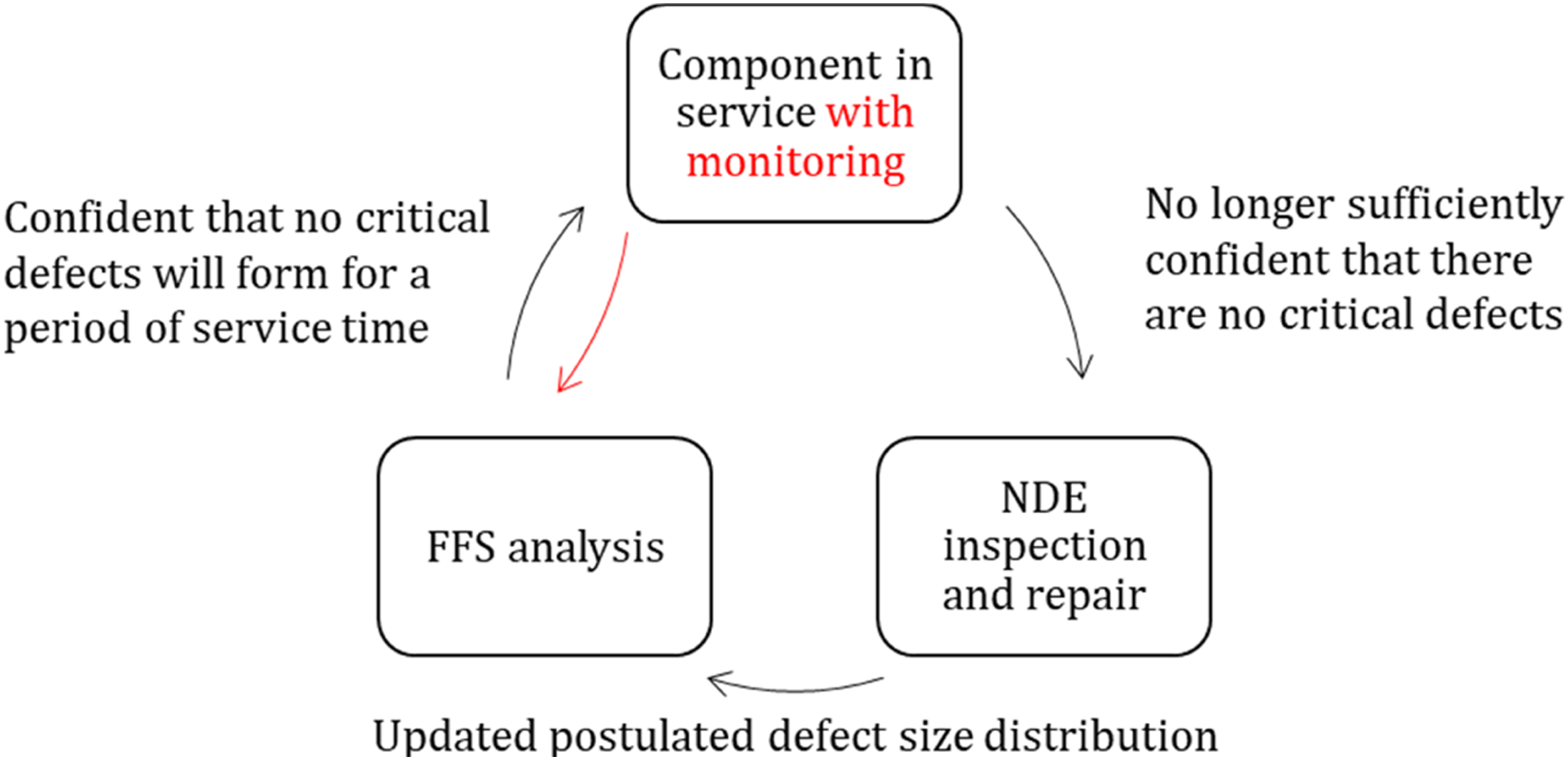

Advances in technology mean that permanently installed monitoring systems for structural health monitoring (SHM) are becoming increasingly viable and attractive. The availability of regular in-situ measurements from permanently installed monitoring systems enables frequent, in-situ assessments of FFS. Figure 1 illustrates the management of an engineering component with monitoring (shown in red) as similarly described in Reference 1. Notably, incorporating data collected from permanently installed monitoring systems has the potential benefit of reducing the need of in-service inspections while ensuring the integrity of the monitored component to the same confidence level. In particular, industrial applications have shown that the deployment of permanently installed monitoring systems is valuable for components that are difficult or hazardous to access and inspect.²

The field of SHM covers a wide variety of technologies and applications, ranging from technologies for global monitoring on a structural level, to the monitoring of localised defects at specific hotspots of an engineering structure.³ Technologies for global monitoring on a structural level include methods for real-time load monitoring for improved structural reliability estimations,^4–6 as well as structural response monitoring using techniques such as vibration-based methods^7,8 and acoustic emissions^9,10 to detect the presence of any substantial damage. Frameworks for probabilistic reliability analysis based on information collected by SHM for global monitoring have also been extensively studied and developed in the literature.^11–14

This research focuses on the use of SHM technologies to monitor more localised defects. Substantial research and development has been carried out recently to develop permanently installed monitoring systems to detect a variety of defects in different engineering applications^15–18 and also how damage growth data can be used for failure prognostics.^19–21 The majority of the research focuses on monitoring the growth of a detected defect where permanently installed monitoring systems are used to size a defect to reduce uncertainty in remnant life predictions. Notably, the use of particle filtering (or sequential Monte Carlo) methods have been used for performing failure prognostics using time-series data due to their versatility in a wide range of applications.^21–23

In many situations, a detectable defect will not be present for the majority of a component’s life and so sizing techniques are not applicable. In this study, it is proposed that binary results (i.e. defect free/defective) can also provide valuable information on the damage state and therefore FFS. Negative measurement results provide evidence that defects of a given size are not present and therefore inform a postulated probability distribution of defects that may be present. This postulated defect distribution then allows for predictions of the remaining useful life of the component using an appropriate defect growth model.

This article proposes a framework that uses a particle filtering method to integrate damage detection data collected from permanently installed monitoring systems into a probabilistic FFS assessment. As schematically illustrated in Figure 2(a), uncertainty in the initial condition, material properties and operating conditions leads to uncertainty in the damage progression and the number of cycles until a limiting damage state is reached. Successive negative monitoring results are used to recursively filter potential cases of substantial damage based on the detection capability of the monitoring system, which is quantified by its POD curve; this is illustrated in Figure 2(b) for a single successive negative measurement. This in turn recursively updates a probability distribution of the number of cycles until a limiting damage state is reached, thus continuously quantifying the FFS of the monitored component.

Figure 2.

Schematic illustrations demonstrating the proposed framework, showing (a) the prediction in failure time given the initial conditions; (b) the prediction in failure time following a negative measurement.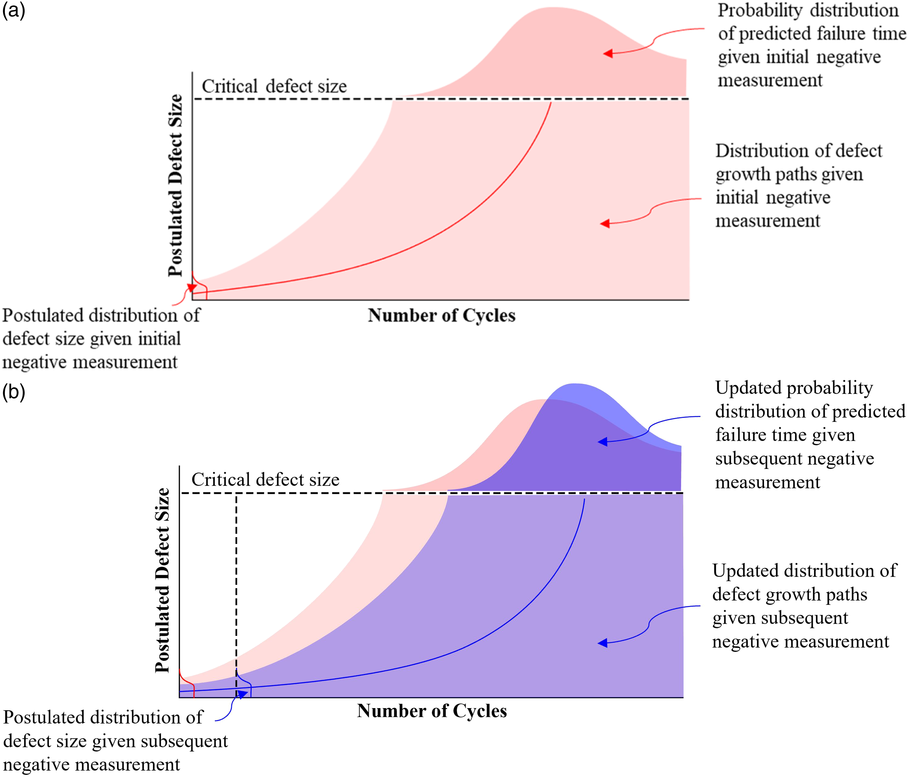

An implementation of the particle filtering approach that takes into account the systematic uncertainty in the detection capabilities of permanently installed sensors is also proposed. As permanently installed sensors are, by definition, fixed in position, uncertainty in the location of the sought defect would result in systematic uncertainty in the detection capability of the sensor. Previous work has demonstrated how to incorporate systematic uncertainties into a receiver operating characteristic (ROC) analysis to quantify the confidence in detection capabilities.²⁴ In this article, these POD curves are used in the particle filtering scheme to postulate possible defect extent.

This article is structured as follows. In the Description of Example Problem section, a description of an example problem that is used to demonstrate the proposed framework is first provided. The theory of particle filtering methods and the subsequent update of probability of failure will be described in the Method section. The particle filtering based FFS assessment approach is then applied to the example problem, with the results being discussed in the Results for the Example Problem section. A method of incorporating the effect of systematic uncertainties on the detection capabilities of permanently installed monitoring systems is demonstrated in the section the Effect of Systematic Uncertainty in the Detection Capability of Permanently Installed Monitoring Systems. Finally, a discussion on the results and conclusions are presented in the Discussion and Conclusions sections.

Description of example problem

To illustrate the proposed framework, a hypothetical example of a steel pipe undergoing three-point fatigue bending is used. The life cycle of the pipe may be managed by one of two approaches. First is the use of periodic inspections only; second is the use of a combination of permanently installed monitoring systems and less frequent manual inspections. Details of the structural problem as well as the inspection and monitoring techniques used in the example problem will be outlined in this section.

Description of the structural problem and damage growth model

A hypothetical example of managing the life cycle of a welded steel pipe with nominal diameter $D = 152.4 mm$ (i.e. 6-inch) and wall thickness $t = 11$ mm undergoing three-point fatigue bending is used in this study. A schematic illustration of the pipe is illustrated in Figure 3. The pipe is welded at the midpoint of the pipe as indicated by the dashed black line in the figure. The pipe is expected to fail through the initiation and propagation of a planar thumbnail fatigue crack at the weld where it experiences maximum stress amplitude.

Figure 3.

Schematic illustration of the welded pipe used in this study. The red line and patch represent the planar thumbnail fatigue crack.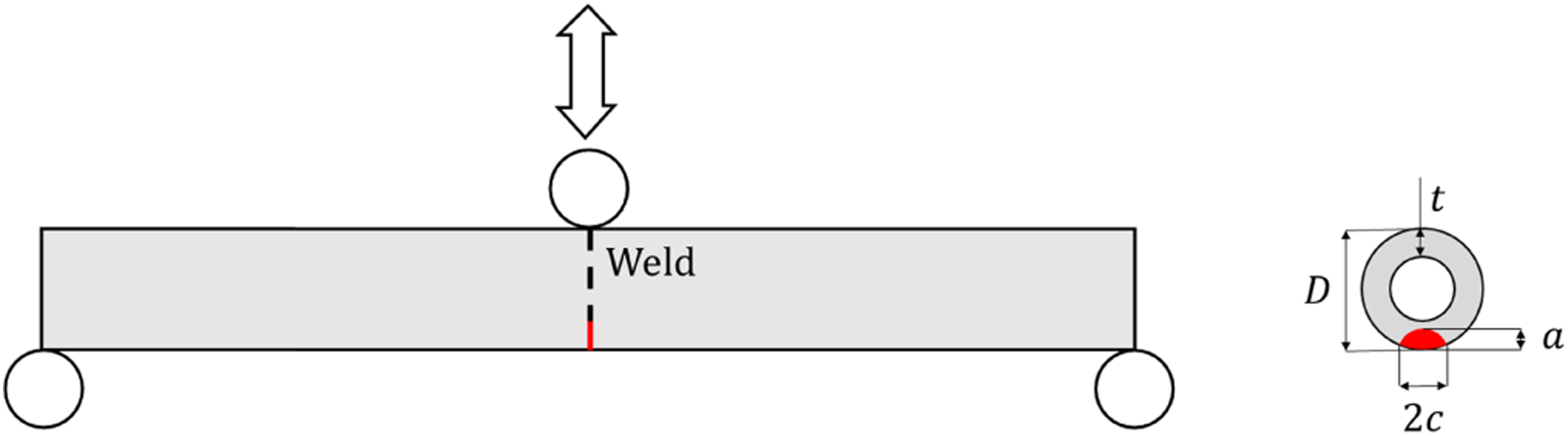

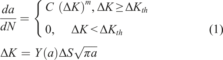
To evaluate the FFS of the pipe, a defect growth model is required. Many empirical fatigue crack growth models are available in the literature. The commonly used Paris’ crack growth law with a cut-off at the threshold stress intensity factor is used in this study as shown in Figure 4 and equation (1); any combination of loading and defect size resulting in $Δ K < Δ K_{t h}$ will not grow. This is consistent with the simplest crack growth model used in the British Standard 7910,²⁵ though the damage model could be replaced with any other. Fracture toughness, $Δ K_{I c}$ , is not considered as it is assumed that the pipe is designed to leak-before-break, meaning that $Δ K_{I c}$ is reached only after a through-thickness crack is formed

\begin{array}{l} \frac{d a}{d N} = {\begin{cases} C {(Δ K)}^{m}, Δ K \geq Δ K_{t h} \\ 0, Δ K < Δ K_{t h} \end{cases} \\ Δ K = Y (a) Δ S \sqrt{π a} \end{array}

(1)

C

and

m

= Paris’ constant and exponent of the material;

Δ K

= stress intensity range;

Δ K_{t h}

= threshold stress intensity range of the material;

a =

defect size in the evaluated defect growth direction;

Y (a)

= geometry factor and

Δ S

= stress range.

Figure 4.

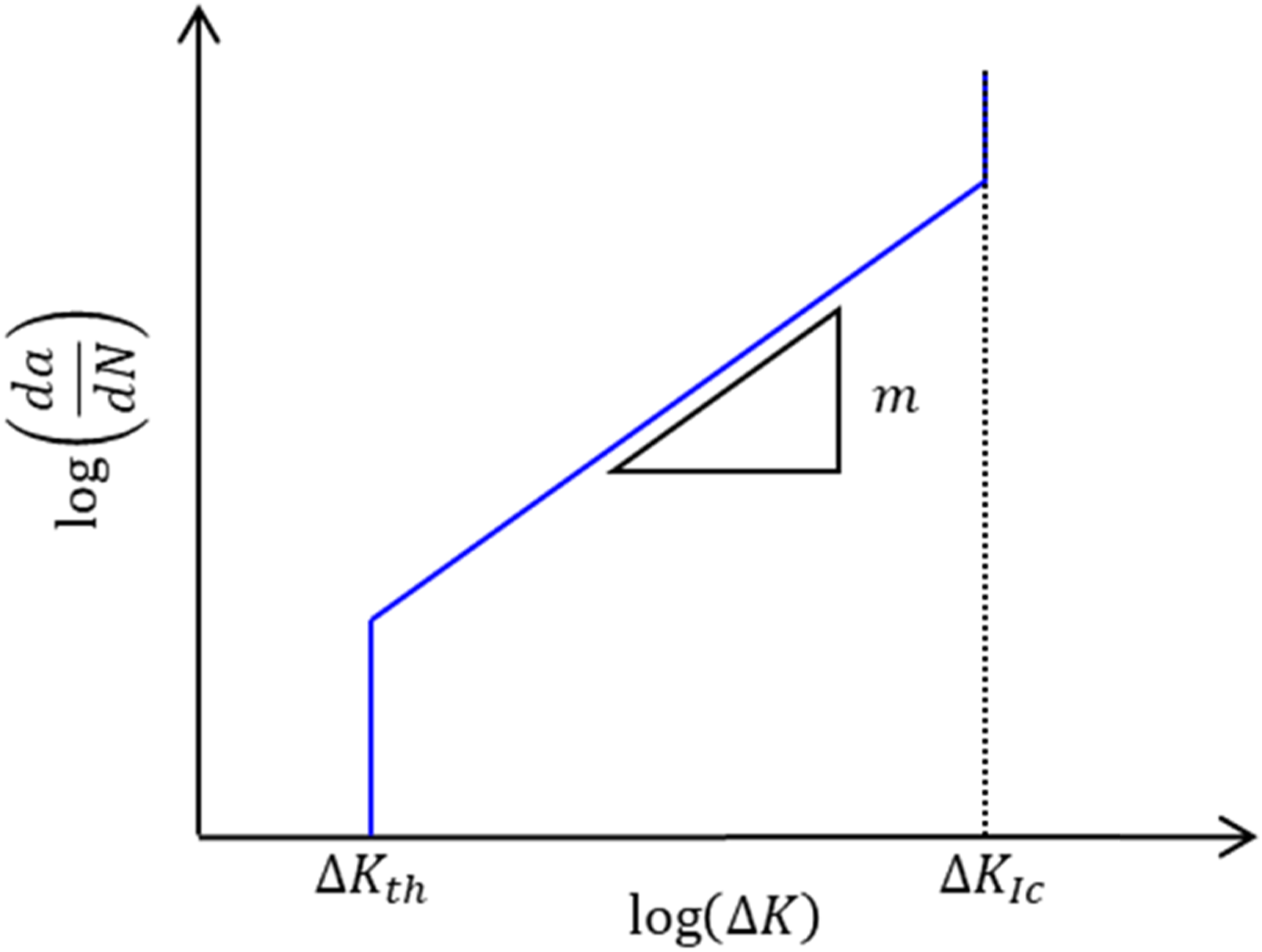
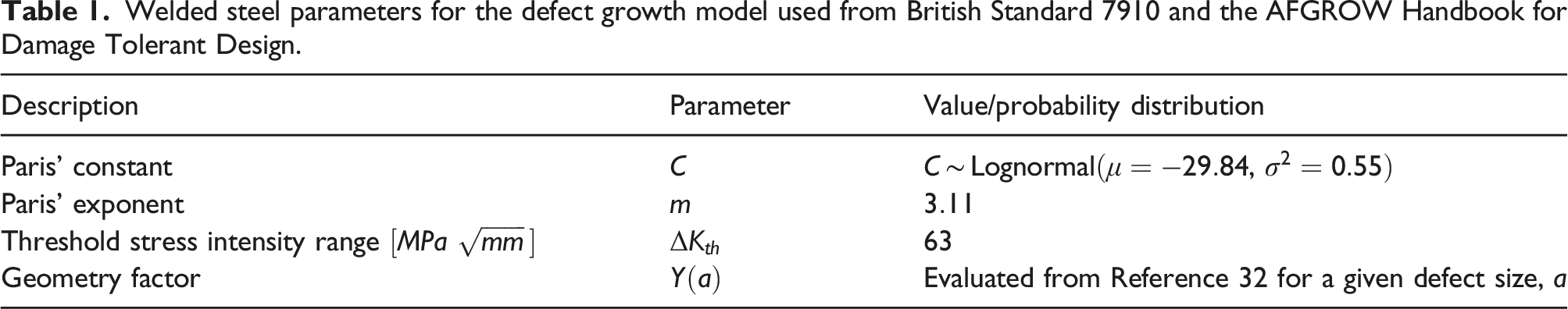
Schematic plot of Paris’ crack growth law with threshold stress intensity factor, $Δ K_{t h}$ , and fracture toughness, $Δ K_{I c}$ .

As with many other damage mechanisms, fatigue crack growth is stochastic in nature.^26–29 In this study, the stochasticity in defect growth is simply represented by a probability distribution of Paris’ constant,

C

, as described in the British Standard 7910.²⁵ Paris’ exponent,

m

, and threshold stress intensity range,

Δ K_{t h}

, are assumed to be known. The values used are again from British Standard 7910²⁵ and are shown in Table 1. While this is clearly a simplified model as pointed out in the literature,³⁰ it is believed that this simplified model is sufficient for illustrative purposes in this study; the approach used here to modelling uncertainty in fatigue is well established in widely accepted standards.^25,31 Moreover, the proposed framework has no theoretical limitations on the complexity of the defect growth model used. Models with more probabilistic variables can easily be substituted as necessary for the specific problem studied, albeit at the cost of requiring more computational power.

Table 1.

Welded steel parameters for the defect growth model used from British Standard 7910 and the AFGROW Handbook for Damage Tolerant Design.

Description	Parameter	Value/probability distribution
Paris’ constant	$C$	$C \sim Lognormal (μ = - 29.84, σ^{2} = 0.55)$
Paris’ exponent	$m$	$3.11$
Threshold stress intensity range $[M P a \sqrt{m m}]$	$Δ K_{t h}$	$63$
Geometry factor	$Y (a)$	Evaluated from Reference 32 for a given defect size, $a$

All postulated initial cracks are assumed to be semi-circular. However, the growth of the semi-circular crack in both the depth, $a$ , and width, $c$ , direction needs to be evaluated. The same defect growth model is used for evaluating the defect growth in both directions; however, the difference in growth rate in the two directions is accounted for when evaluating the geometry factor, $Y (a)$ , as described in the AFGROW Handbook for Damage Tolerant Design.³²

The uncertainty in loading conditions experienced by the component is characterised by uncertainties in stress range, which is said to follow a normal distribution with parameters shown in Table 2. Loading is assumed to be fully reversed (i.e. load ratio,

R = - 1

). The loading conditions here are again a simplified model and assumes that the loading is a stationary process and can be approximated as a single equivalent stress range similar to References 30 and 33. In practice, there are situations where loading conditions may be nonstationary, meaning that loading conditions may vary with time. This will have to be accounted for when performing predictions in defect growth. Potential approaches for a more realistic representation of the loading conditions such as using on-load data^4,34,35 can be substituted as needed.

Table 2.

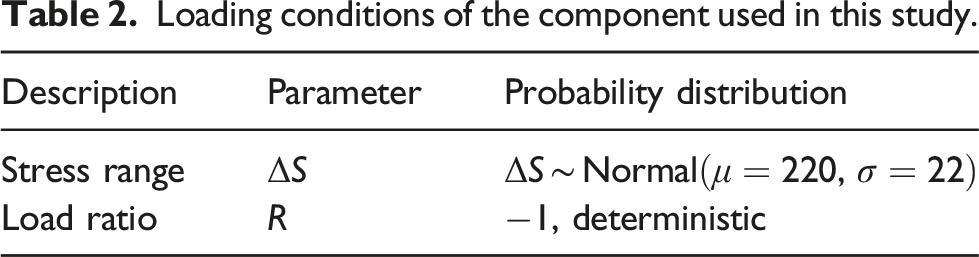
Loading conditions of the component used in this study.

Description	Parameter	Probability distribution
Stress range	$Δ S$	$Δ S \sim Normal (μ = 220, σ = 22)$
Load ratio	$R$	$- 1$ , deterministic

With the loading conditions and defect growth parameters defined, defect growth may be modelled and predicted by numerically integrating the crack growth law. A sample deterministic result of a $1$ mm semi-circular crack (i.e. $a = c$ ) taking $N_{f}$ cycles to grow to a through-thickness crack (i.e. $a = t$ ) with mean values of Paris’ constant, $C$ , and stress range, $Δ S$ , is shown in Figure 5. The uncertainty in these parameters and the postulated crack length will result in a range of possible defect growth curves; this uncertainty and how it is managed with inspection and monitoring results is the focus of this research.

Figure 5.

Sample result of fatigue crack growth, showing (a) growth in the depth (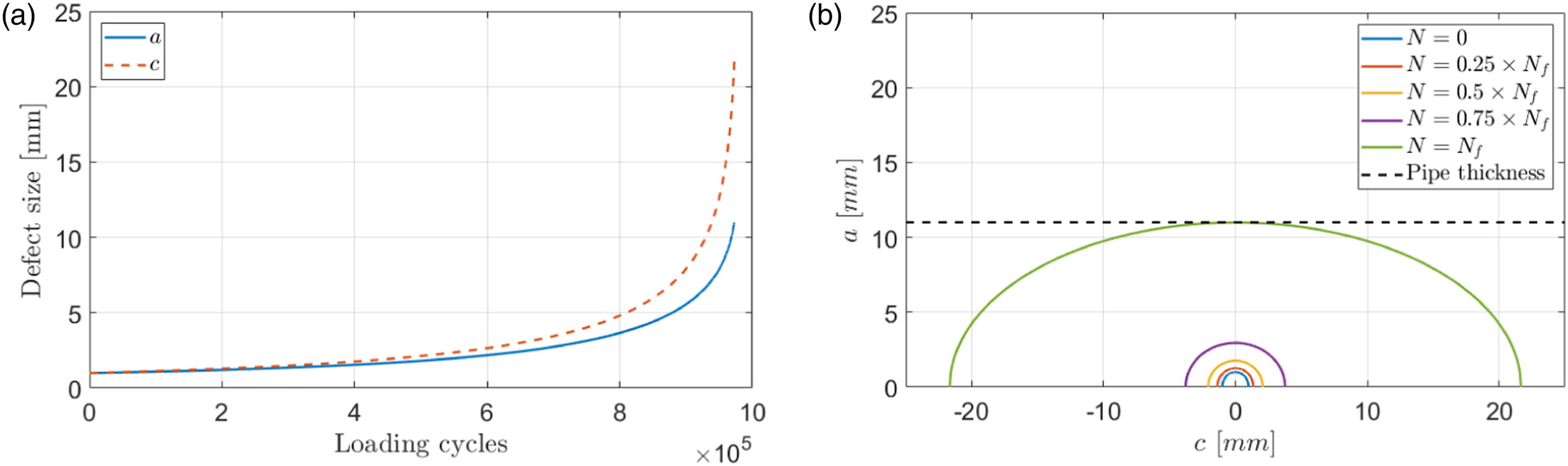 $a$ ) and width ( $2 c$ ) direction against the number of cycles; (b) shape of the defect at selected intervals.

Description of the inspection and monitoring schemes

Although the measurement technology is arbitrary, in this example problem an eddy current sensor will be considered for periodic manual inspections, and a permanently installed ultrasonic guided wave sensor will be used for defect monitoring. The POD curves of the two sensors are shown in Figure 6; descriptions of the setup and detection capability of the two sensors are given in the following sections.

Figure 6.

POD curve of (a) the eddy current sensor and (b) the guided wave sensor used in this study.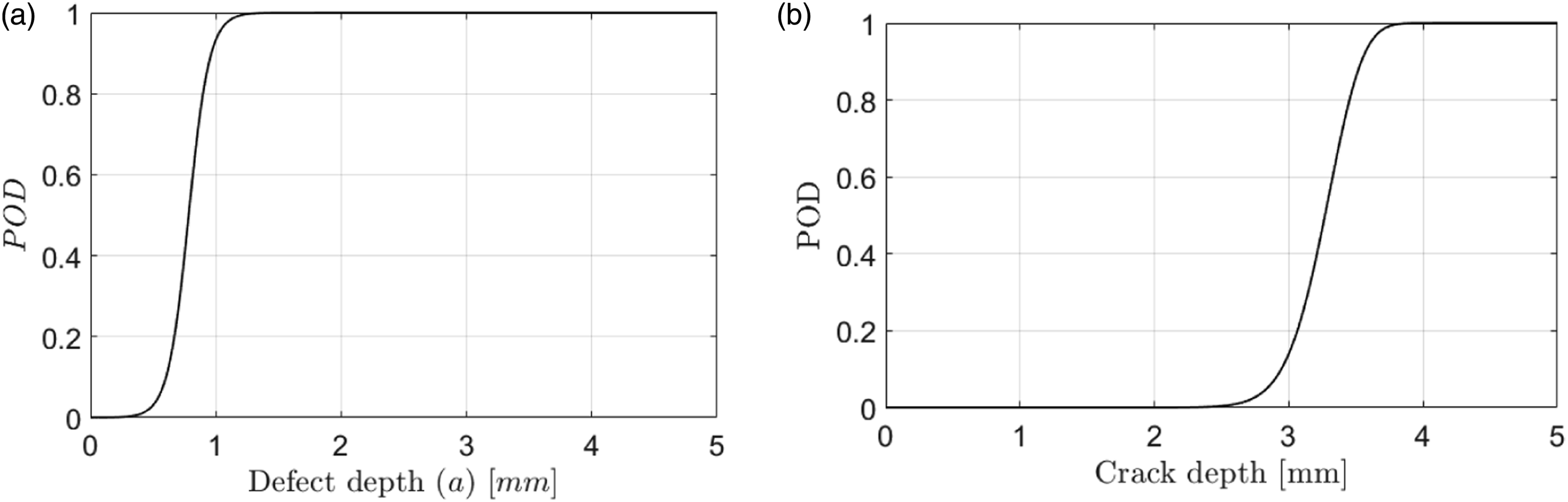

Eddy current sensor for inspection

An eddy current sensor is considered for manual inspection in this study. The POD curve of the eddy current sensor for a crack-like defect is obtained from existing literature for an eddy current sensor by Mohseni et al.³⁶ where its detection capabilities are evaluated experimentally with qualified inspectors and fitted to a logistic function. Though this POD study was done on steel plate structures instead of pipes, it provides a reasonable estimate on the typical detection capabilities of an eddy current sensor. The aim here is to demonstrate the framework, and the numerical results produced is not intended to be used in any real-life problems. A more thorough POD study will certainly be needed when applying the framework to assessments in real-life.

As a metric of detection capability, the eddy current sensor is expected to have a $POD = 90 %$ at $a = 0.95$ mm (no probability of false alarm, PFA, reported in the study).

Guided wave sensor for monitoring

For defect monitoring, a short-range shear-horizontal guided wave permanently installed monitoring system as described in Reference 18 is considered. The POD curve of the guided wave sensor is evaluated using a combination of analytical solutions and experimental results produced by Chua et al.^18,37 A separate study on long-term stability of guided wave systems also yielded similar results in terms of signal noise level.³⁸ A low target PFA of $10^{- 6}$ is used. This is necessary for monitoring systems as frequent measurements are taken. If a higher target PFA is used, it is expected that a false alarm would occur at some point within the service life of the monitored component given the frequent measurements, resulting in unnecessary and potentially costly outages.

As a metric of detection capability, the guided wave sensor has a $POD = 90 %$ at $a = 3.5$ mm. This is inferior compared to the eddy current sensor used for inspections but has the benefit of being permanently installable with greater area coverage and therefore ability to take frequent readings to monitor the entire pipe.

Method

This section details the framework proposed in this research to integrate damage detection data collected from both inspections and permanently installed monitoring systems to perform probabilistic FFS assessments. It is important to note that only sources of random uncertainty from the inspection and monitoring systems will be considered in the analysis in this section; this implies that all measurements are assumed to be independent. An extension of this method to incorporate sources of systematic uncertainty in the monitoring systems will be discussed in the section the effect of systematic uncertainty in the detection capability of permanently installed monitoring systems.

Bayesian inference for a single measurement result

In this study, we are seeking to determine the probability of a defect of postulated severity (i.e. defect size), $a$ , being present following a negative measurement. It is worth emphasising that this distribution of postulated defect size is different to the distribution of the size of a detected defect. A negative measurement only eliminates the possibility of what sized defects are not present. The distribution therefore estimates what sized defects may be present in the component of interest, rather than the size of an actual detected defect.

A negative measurement occurs when the output of the inspection or monitoring system, $X$ , is less than a specified threshold value $X_{t h}$ , which is typically defined based on requirements on the probability of a false alarm. This postulated defect size distribution is thus expressed as

P (a | X \leq X_{t h})

(2)

and can be estimated using Bayes’ theorem

P (a | X \leq X_{t h}) \propto P (a) \times P (X \leq X_{t h} | a)

(3)

The distribution $P (a | X \leq X_{t h})$ is the posterior and is evaluated as the product of the prior distribution, $P (a)$ , and the likelihood function derived from measurements, $P (X \leq X_{t h} | a)$ .

The prior distribution, $P (a)$ , describes the estimated defect size distribution prior to any measurements being made. Manufacturing standards or previous inspections may indicate that defects above a certain size are not present. In this study, a naïve, uniform distribution from zero to full thickness will be conservatively assumed as the starting point: $P (a) \sim Uniform (0, t)$ .

The distribution $P (X \leq X_{t h} | a)$ is the likelihood function. The sensor output, $X$ , for an arbitrary measurement of a given defect severity, $a$ , can be represented by a probability distribution function due to random uncertainties in the measurements; this is shown in Figure 7 for a single defect size. The sought likelihood function is simply the probability of a false negative as a function of defect size, $PFN (a)$ , as illustrated in Figure 7

PFN (a) = P (X \leq X_{t h} | a)

(4)

Figure 7.

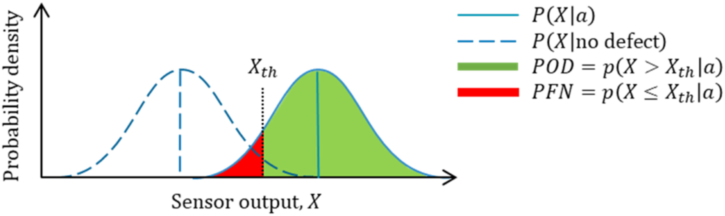
Schematic illustration of the probability distributions of the system output, $X$ , for a defect-free case, $P (X | no defect)$ , and when a defect of size $a$ is present, $P (X | a)$ . The threshold, $X_{t h}$ , is a chosen value which a detection is called when the inspection or monitoring outputs $X > X_{t h}$ . The area shaded in green represents the probability of detection for a defect of size $a .$ The area shaded in red represents the probability of a false negative for a defect of size $a$ .

In this study, $PFN (a)$ will be expressed in terms of the closely related and more commonly evaluated probability of detection curve, $POD (a)$

P (X > X_{t h} | a) = 1 - P (X \leq X_{t h} | a)

(5)

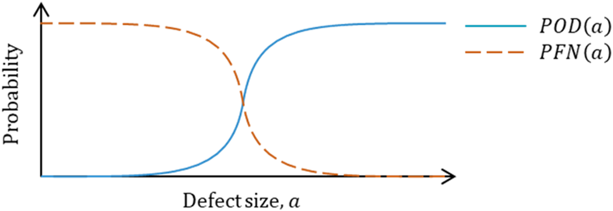
Or in alternative notation

POD (a) = 1 - PFN (a)

(6)

as illustrated in Figure 8. Therefore, the likelihood is simply

P (X \leq X_{t h} | a) = 1 - POD (a)

(7)

Figure 8.

Schematic illustration of a probability of detection (POD) curve and its corresponding probability of false negative (PFN) curve.

The postulated defect size distribution can now be estimated as the product of the prior and the likelihood as illustrated in Figure 9. The probability density function will need to be normalised so that it integrates to unity. This posterior distribution gives an updated estimation of defect size distribution based on the inspection or monitoring result. The posterior postulated defect size distribution only contains negative information providing information of what size defects are not present. It is worth noting how the posterior distribution takes the same shape as the likelihood function in Figure 9. This is due to the fact that a naïve prior is being used; this will not be the case if a different prior is used. With the use of a naïve prior, the probability distribution function is flat as $a \to 0$ ; there is equally no evidence to suggest whether a defect is present or not over this range. This will ultimately result in conservative estimates of probability of failure.

Figure 9.

Schematic illustration of how the posterior postulated defect size distribution is formulated based on the naïve prior and likelihood from the POD curve.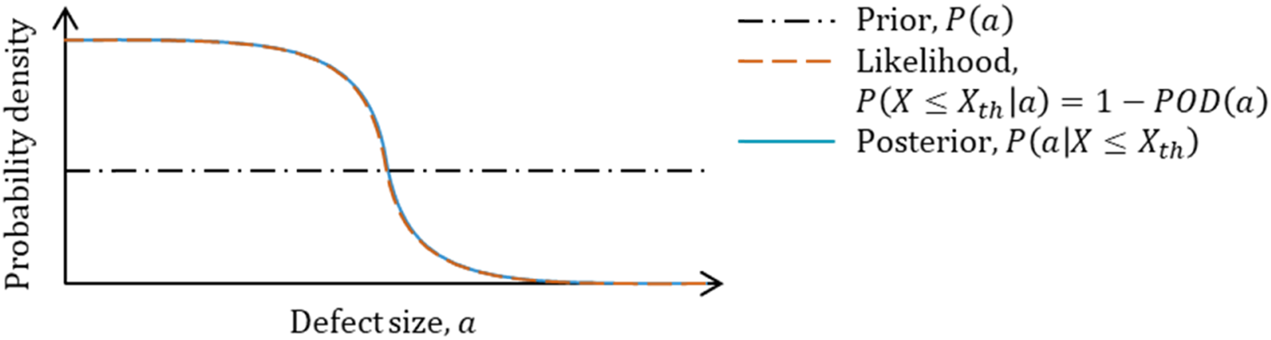

Particle filtering for repeated measurements

The previous section outlined the use of the POD curve to infer possible defect sizes from a single measurement. In practise, multiple inspections are performed, and if permanently installed monitoring systems are used, measurements are frequently collected throughout the service life of the component. Each new measurement should inform the possible defect sizes. The process of updating the distribution of defect sizes is not as straightforward as recursively applying Bayes’ theorem by using the previously evaluated posterior distribution as the prior distribution for the latest measurement. This is because the size of any potential defect in the component would evolve with time.

As a result, a dynamic state-space modelling approach is required. Particle filtering methods (also known as sequential Monte Carlo methods) are of growing popularity for probabilistic damage prognosis in multiple applications given their flexibility and ease of implementation and will be used in this study.^21,39,40 The theory of particle filtering methods is widely discussed in existing literature; a summary of the method is given here in the context of managing the life cycle of engineering components. The aim is to evaluate the defect size distribution after $N$ loading cycles given all available inspection and monitoring results. This is expressed as

P (a_{j} | M_{0 : j})

(8)

$a_{j}$ = Size of defect at the most recent, $j$ -th inspection or monitoring result.

$M_{0 : j}$ = Vector of results of the zeroth to $j$ -th measurement from inspection or monitoring, the zeroth being the initial measurement prior to service (i.e. at $N = 0$ ). A binary result is considered; either no defect is detected (i.e. $X \leq X_{t h}$ ) or a defect is detected (i.e. $X > X_{t h}$ ).

The overall process is illustrated in Figure 10, with the individual steps outlined in the following text.

Figure 10.

Illustration of the particle filtering approach to recursively update the defect size distribution given inspection or monitoring results. Numbers in orange circles represent the corresponding steps.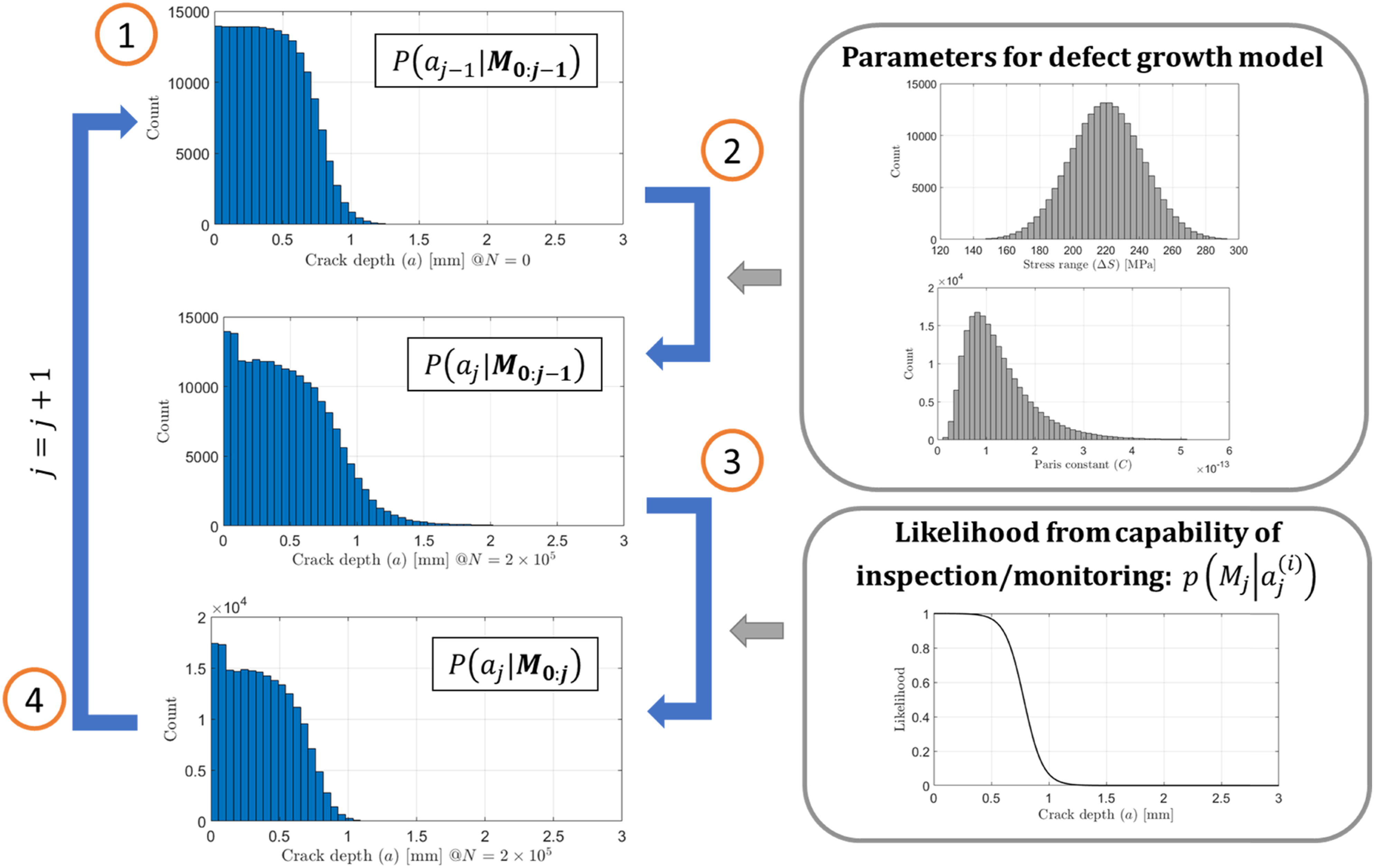

Step 1

Specify the prior

To initiate the process, a distribution of postulated initial defect size, $P (a_{0})$ , would have to be defined. In numerous studies of probabilistic damage prognosis using defect growth models, the assumption that a macroscopic defect is already present and detected is often made.^20,41 Under such conditions, the initial defect size distribution would simply be the measured defect size together with its quantified uncertainty. However, there are also cases where the component of interest is nominally ‘defect-free’. For such cases, a postulated defect size distribution would have to be used.

There are numerous approaches to postulating the initial defect size distribution. One approach is the use of an equivalent initial flaw size; this approach uses the defect growth model to backward-extrapolate the equivalent initial flaw size such that the evaluated component life matches that evaluated using the stress-life approach.⁴² Alternatively, the postulated initial defect size distribution can be defined in view of knowledge from ‘service experience, the manufacturing process, resolution limits of a NDE technique’.⁴³

As previously discussed in the Bayesian Inference for a Single Measurement Result section, in the example problem the prior will initially be a naïve uniform distribution. However, the negative result of an inspection prior to service will immediately filter out the probability of the presence of defects larger than the detection capability of the inspection as illustrated previously in Figure 9; thus

P (a_{0} | M_{0}) \propto 1 - POD (a)

(9)

where

M_{0}

is the negative result of the initial inspection. Using the POD curve of the eddy current sensor defined in the Eddy Current Sensor for Inspection section,

P (a_{0} | M_{0})

is obtained by normalising the function

1 - P O D (a)

for

a \geq 0

such that it integrates to unity. This is used as the distribution of the size of a postulated defect that may be present in the component given the negative result of the initial inspection.

Step 2

Time dependence of defect evolution

From one measurement to the next, any postulated defects would have likely grown in size. It is therefore necessary to evaluate the evolved distribution according to the assumed defect growth model. At the instance where the $j$ -th measurement is made, the previous measurement would be the $(j - 1)$ -th measurement, and the previously evaluated defect size distribution would be $P (a_{j - 1} | M_{0 : j - 1})$ . The aim of this step is to evaluate the distribution $P (a_{j} | M_{0 : j - 1})$ with the defect growth model. This distribution will act as the prior distribution in the following step.

A Monte Carlo approach is used to evaluate the evolved defect size distribution. An appropriate sampling method such as the Latin hypercube sampling method⁴⁴ used in this study is used to draw $i = 1, \dots, U$ samples (or particles) from the distribution $P (a_{j - 1} | M_{0 : j - 1})$ and other parameters with uncertainties of the defect growth model (i.e. Paris’ constant, $C$ , and stress range, $Δ S$ , in the example problem). Each sample of defect size, $a_{j - 1}^{(i)}$ , and a set of probabilistic parameters of the defect growth model is then used to evaluate each corresponding $a_{j}^{(i)}$ . This can then be represented as a histogram of evolved defect sizes which approximates the distribution $P (a_{j} | M_{0 : j - 1})$ .

An illustration of evaluating the defect size distribution from the example problem is shown earlier in Figure 10. From the results, it is clear that a significant portion of the postulated defects have grown in size. Note that a portion of smaller defects did not evolve; this is due to the fact that the combination of defect size and defect growth parameter results in stress intensity is below the growth threshold (see equation (1)).

Step 3

Particle filtering using the POD curve

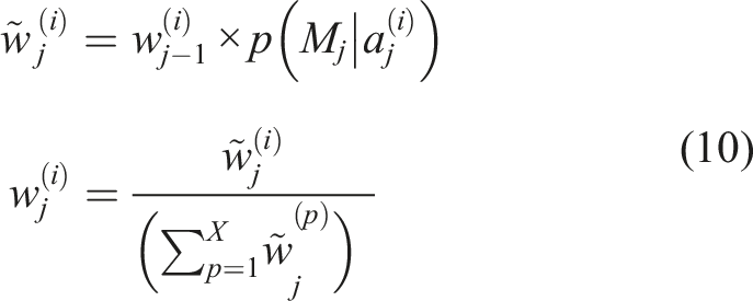
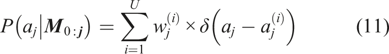
With the distribution $P (a_{j} | M_{0 : j - 1})$ evaluated, the next step is to incorporate the latest measurement result, $M_{j}$ , and thus obtain the distribution $P (a_{j} | M_{0 : j})$ . To do so, each sample of $a_{j}^{(i)}$ is assigned a weight, $w_{j}^{(i)}$ , evaluated as

\begin{array}{l} {\tilde{w}}_{j}^{(i)} = w_{j - 1}^{(i)} \times p (M_{j} | a_{j}^{(i)}) \\ w_{j}^{(i)} = \frac{{\tilde{w}}_{j}^{(i)}}{(\sum_{p = 1}^{X} {\tilde{w}}_{j}^{(p)})} \end{array}

(10)

where

w_{j - 1}^{(i)}

is the previously evaluated weight of the particle and

p (M_{j} | a_{j}^{(i)})

is the likelihood of the measurement result for sample

i

evaluated using equation (7) with the POD curve of the latest measurement. This describes the likelihood of obtaining the latest measurement result if a defect of size

a_{j}^{(i)}

is indeed present. With this, the posterior distribution,

P (a_{j} | M_{0 : j})

, that describes the updated postulated defect size given all previous inspections and the current inspection can be approximated as

P (a_{j} | M_{0 : j}) = \sum_{i = 1}^{U} w_{j}^{(i)} \times δ (a_{j} - a_{j}^{(i)})

(11)

where

δ (\cdot)

is the Dirac delta function. Again, an illustration of the process for the example is shown earlier in Figure 10.

Step 4

Resampling (optional) and updating

Typically when performing particle filtering, resampling is performed using the posterior distribution, $P (a_{j} | M_{0 : j})$ ; methods to conduct resampling can be found in Reference 45. This process is to avoid sample degeneracy where more and more samples have a weight of zero, resulting in fewer useful samples. However, it is known that standard methods of resampling would reduce the variance in samples as explained in Reference 46; the effect is known as sample impoverishment. This is particularly undesired for this specific application since the extreme cases are of great importance when evaluating the FFS of components. With reduced variance in samples, postulated defects of significant sizes are likely to be removed, resulting in a non-conservative estimate in FFS.

Therefore, resampling is not used in this study; an appropriate number of samples are used to ensure that there are sufficient non-zero weight samples throughout the evaluation process to provide accurate results; $2 \times 10^{6}$ samples were used in the study of the example problem. A potential alternative is to use more advanced resampling techniques such as deterministic resampling which are designed to minimise the effect of sample impoverishment.⁴⁷

Finally, the weighted (or resampled) samples from $P (a_{j} | M_{0 : j})$ are then used in the next iteration of the process when a new data point from inspection or monitoring is obtained (i.e. $j = j + 1$ ) and the process recursively updates the defect size distribution.

Forecasting estimated probability of failure

Once a distribution of the postulated defect size has been evaluated, it is possible to forecast the distribution forwards using the assumed damage model and Monte Carlo methods. With this, the probability distribution of the number of cycles until a chosen critical severity, $P (a = a_{c r i t})$ , can be estimated as illustrated in Figure 11. The probability that a defect exceeds the critical severity as a function of number of loading cycles is termed the probability of failure, $POF (N)$

POF (N) = p (a \geq a_{c r i t} | M_{0 : j}, N)

(12)

Figure 11.

Plot of the results of forecasting the distribution forwards using the assumed damage model and Monte Carlo methods.

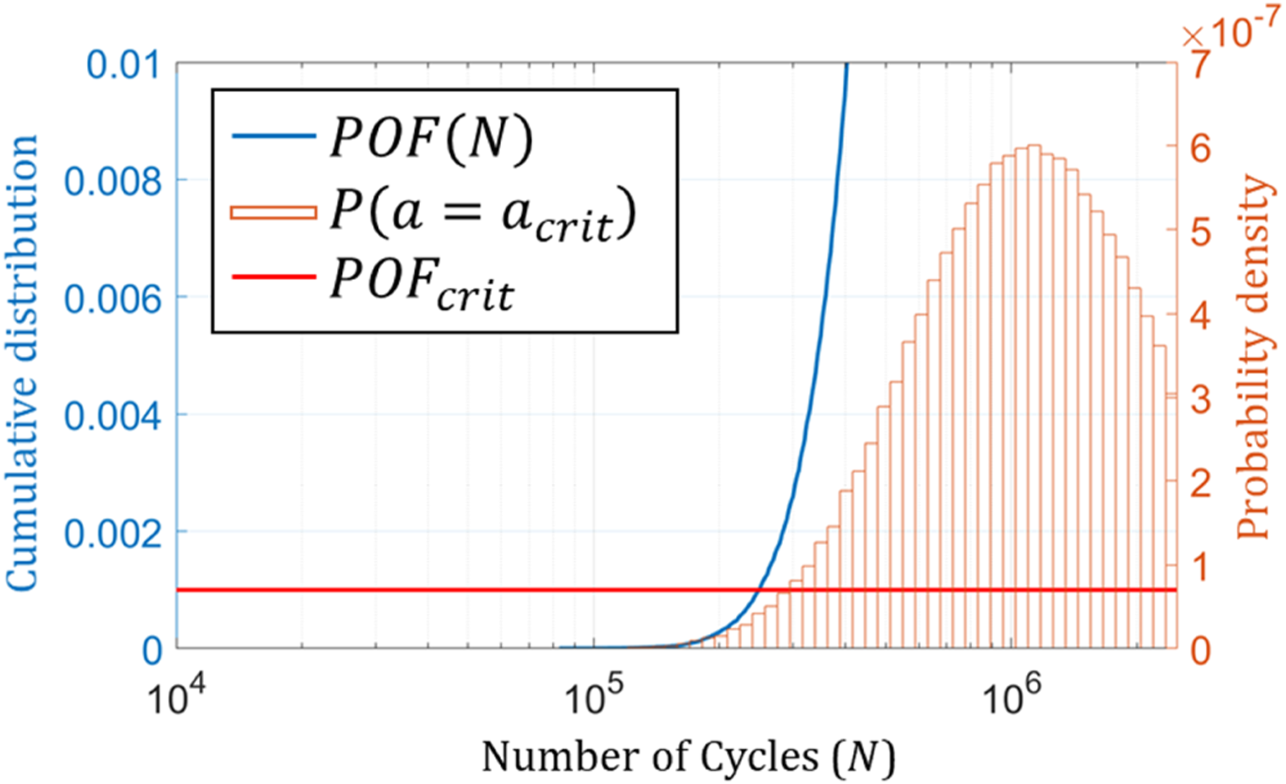
The fitness-for-service can be evaluated in terms of the probability of failure. A maximum allowable probability of failure is set, $PO F_{c r i t}$ . This maximum acceptable probability of failure depends on the specific application and is typically governed by the consequence and cost of a failure as specified in codes and standards.^25,31

It is worth considering the nature of the distribution $POF (N) = p (a \geq a_{c r i t} | M_{0 : j}, N)$ and how it updates following a negative inspection or monitoring result. Clearly, as the number of loading cycles increases, the probability of failure will increase as demonstrated by the plot of $POF (N)$ in Figure 11. A negative inspection or monitoring would result in a reduction in the probability of failure since the most severe postulated defects would be eliminated; this was illustrated earlier in Figure 2. This reduction in probability of failure is not because an inspection or monitoring has somehow had a material effect on the longevity of the asset, but rather the new information has updated the predicted distribution of when the asset will reach the critical failure condition.

Inspection decision and updating

Typical opportunities to inspect the component are governed by a calendar or usage-based maintenance scheme. In Figure 12, arbitrary opportunities for inspection, $N_{1}$ , to $N_{4}$ , are shown and represented as dot-dash grey lines. In this study, a new inspection is said to be required if the predicted probability of failure (shown in black dashed lines in Figure 12) is predicted to rise above the critical probability of failure before the next inspection opportunity. In Figure 12, an inspection is conducted at time $N_{2}$ to update the estimated probability of failure (shown as the dash green line). Given a negative inspection result, $POF$ at $N_{2}$ becomes zero, and postulated defects that may have been missed by the inspection are propagated to update the estimated $POF (N)$ curve. This is similar to that illustrated in standards and recommended practices on how inspection results update the estimation in probability of failure.³¹

Figure 12.

Schematic plot of how 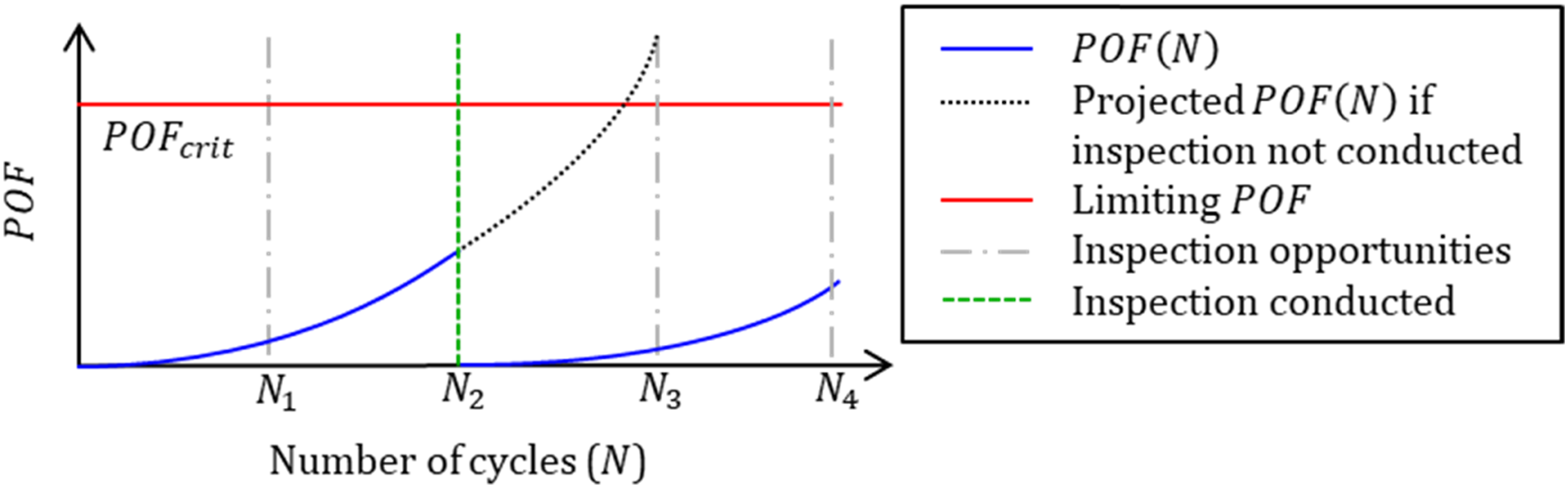$POF (N)$ evolves with time and updated with inspections.

If monitoring is used, then predictions of the probability of failure are based on the assumption that no measurements will be available before the next inspection, even if permanently installed sensors are present; this is necessary to provide an equivalent comparison to only having inspections. These trajectories are only used to decide if an inspection is required. In practise, the estimated probability of failure will follow a different trajectory depending on future positive or negative monitoring results.

Results for the example problem

The previous sections detailed the process of updating the distribution of possible defect sizes and evaluating the FFS of the component. Using the process detailed, simulations can be conducted to illustrate how the estimated probability of failure evolves over time when managed by inspection only or a combination of inspection and monitoring.

Recall from the Description of Example Problem section that we are considering a pipe undergoing three-point fatigue bending that is susceptible to the initiation and propagation of a planar thumbnail fatigue crack. It is assumed that the pipe is designed to leak-before-break, so the failure criterion is defined as having a through-wall crack (i.e. $a_{c r i t} = t$ ). The maximum acceptable probability of failure, $PO F_{c r i t}$ , is set as $10^{- 3}$ in this study. It is assumed that there is an opportunity to inspect the component every $10^{5}$ loading cycles.

Evaluation on the number of inspections required is conducted for the first $2 \times 10^{6}$ loading cycles. The case where all inspections and data from permanently installed monitoring systems return a negative result is considered, which is reasonable since the median loading cycles to failure of the component is estimated to be $2.2 \times 10^{6}$ cycles when evaluated using the material properties and loading conditions defined in the Description of Example Problem section and initial postulated defect size distribution in the Particle Filtering for Repeated Measurements section. The aim is to minimise the required number of inspections. Two management schemes are considered: the first is when only periodic inspections are used and the second is when a combination of inspections and monitoring is used.

Integrity assessment with inspections only

We begin by looking at the scenario where only in-service inspections are used to manage the welded pipe. The plot of estimated probability of failure against the number of loading cycles, $N$ , is shown in Figure 13; this is equivalent to the schematic illustration shown earlier in Figure 12. It can be seen that for the first $6 \times 10^{5}$ cycles, an inspection is required every $2 \times 10^{5}$ cycles as indicated by the dashed green lines. However, with successive negative inspection results, the possibility is that significant defects that would have grown to a detectable size are filtered out. Equally, the probability that there are only small defects below the crack growth threshold increases. Thus, an inspection is only required every $3 \times 10^{5}$ cycles after the third in-service inspection and every $4 \times 10^{5}$ cycles after the fifth in-service inspection. Overall, in this specific scenario, a total of six in-service inspections are required for the managed component to safely operate for $2 \times 10^{6}$ cycles assuming all inspections return a negative result.

Figure 13.

Evolution of confidence in FFS (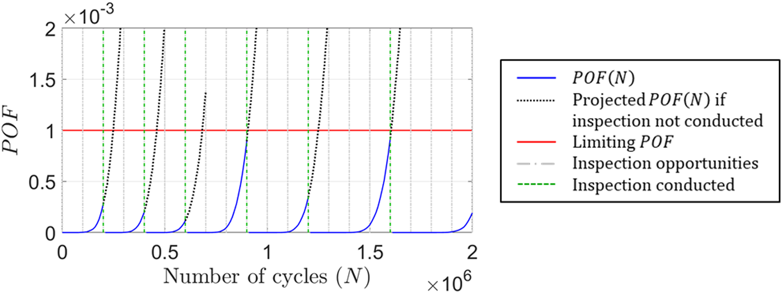 $FF S_{C}$ ) throughout the life cycle of the managed component using only periodic inspections. A total of six in-service inspections are required for the component to last $2 \times 10^{6}$ cycles.

Integrity assessment with inspections and monitoring

We now proceed to consider the scenario where a permanently installed monitoring system is installed on the welded pipe. It is assumed that monitoring data are collected every $10^{4}$ cycles, which translate to 10 measurements between each inspection opportunity. The plot of $POF$ against $N$ for the case where a monitoring system is incorporated is shown in Figure 14. Given that the permanently installed monitoring system has a $POF$ of unity for a defect of the critical size (i.e. $POF (a_{c r i t}) = 1$ ), the estimated probability of failure immediately after a negative result from the monitoring system would always be zero. Therefore, since the reduction in confidence between the frequent measurements is negligible, $POF$ effectively remains constant at zero throughout if all monitoring results are negative.

Figure 14.

Evolution of confidence in FFS (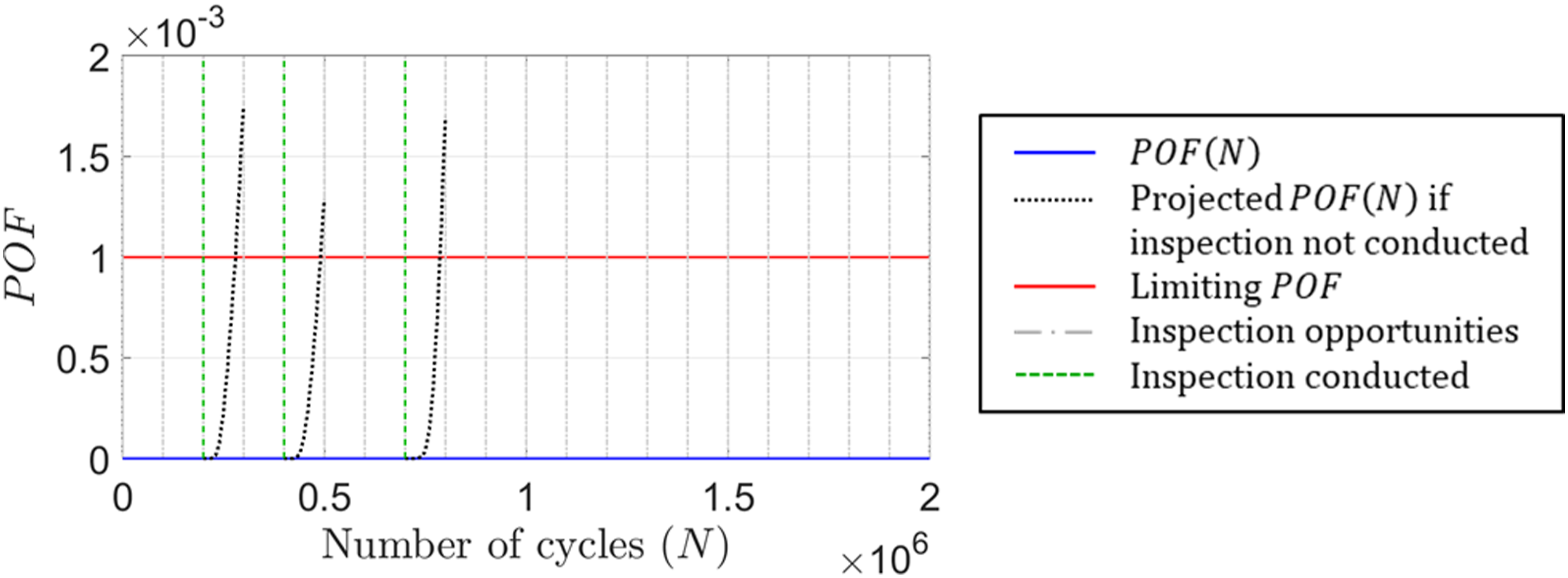 $FF S_{C}$ ) throughout the life cycle of the managed component using inspections and monitoring. A total of three in-service inspections are required for the component to last $2 \times 10^{6}$ cycles.

However, it can be seen that the projected $POF$ may still rise above $PO F_{c r i t}$ as projections of $POF$ are based on the assumption that no future monitoring measurements are available. At 2, 4 and $7 \times 10^{5}$ cycles in this specific scenario, the projected $POF$ would exceed $PO F_{c r i t}$ before the next available inspection opportunity as indicated by the dash black lines in Figure 14; an inspection is therefore required.

It can be seen from the results that in this particular example the value of having a monitoring system installed is relatively limited during the early stages of component life. Recall that the detection capability of the monitoring system is inferior compared to the inspection technique ( $POD = 90 %$ at $a = 3.5$ mm and 0.95 mm, respectively). As a result, there is insufficient information to completely eliminate the possibility of significant defects being present and to keep the $POF$ below the desired level. This means that an inspection is required after 2, 4 and $7 \times 10^{5}$ loading cycles, which is nearly identical to the case where only inspection is used.

As more measurements with negative results are obtained, there is greater confidence in the fitness-for-service of the component, and thus an inspection is no longer required from $7 \times 10^{5}$ cycles onwards. This increase in confidence of the integrity of the component is a consequence of the fact that there is an increase in confidence on the combination of material properties, loading conditions and size of any defects present. On the one hand, if an extreme combination of these parameters is true for the monitored component, the defect would have already grown to a detectable size. As no defects have been detected, these combinations of model parameters are filtered out, updating the estimated distributions of the model parameters. Conversely, it is also increasingly likely that defects present are below the size required for growth. Referring to the damage growth model described earlier in equation (1) and Figure 4, it is increasingly likely that no cracks are present that will result in defect growth given the combination of loading conditions, material properties and defect size (i.e. $Δ K \geq Δ K_{t h}$ ). As a result, the weighted histogram becomes bimodal at $N = 10^{6}$ as illustrated in Figure 15 where the weighted histograms of the size of the sampled postulated defects at $N = 0$ and $N = 10^{6}$ cycles are plotted. This effect is also observed in the example analysis of existing standards for probabilistic inspection planning in DNV-GL-C210³¹ where simple Bayesian updating is used.

Figure 15.

Weighted histograms of the sampled postulated defect sizes at (a) 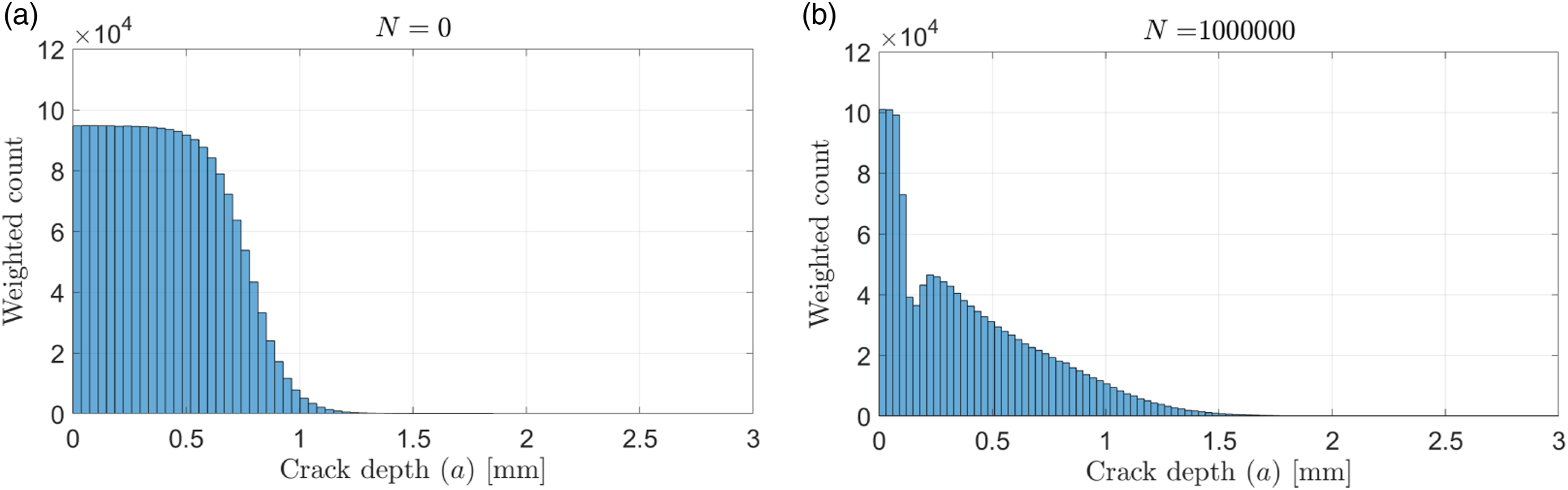$N = 0$ and (b) $N = 10^{6}$ cycles.

In this specific example, the results show that introducing the monitoring system reduced the number of required inspections from six to three. This result is dependent on the detection capabilities of the inspection and monitoring system. It was found that a monitoring system with $POD = 90 %$ at approximately $a = 2.5 m m$ would completely eliminate the need of in-service inspections as the possibility of a significant defect would be kept sufficiently low for $POF$ to remain below the desired level.

The effect of systematic uncertainty in the detection capability of permanently installed monitoring systems

So far in this study, the uncertainties in the sensor outputs are well characterised and only considers random sources of uncertainty. Consequently, the POD curves used are themselves deterministic, suggesting that a certain POD is assured for a given damage severity. In reality, a number of sources of systematic effects can cause uncertainty in the POD curves, warranting a probabilistic treatment. Systematic effects are especially acute in permanently installed sensors which are in a fixed location.^48,49 Most notably, the probability of detection may be highly dependent on the relative position between the installed sensor and the sought defect⁴⁹; if the sought defect happens to occur outside the field of sensitivity of the installed sensors, the probability of detection is going to be severely compromised. Other examples of sources of systematic uncertainty are any imperfections and dynamic responses of the beam that would alter the sensor output, defect morphology⁵⁰ and the quality of the coupling between the sensor and the component.⁵¹ The possibility that negative measurements are a consequence of unfavourable systematic effects such as a defect occurring outside of the field of sensitivity must be taken into consideration.

Particle filtering incorporating uncertainty in POD curve

An implementation of the particle filtering approach which incorporates the effect of systematic uncertainty in the detection capability of permanently installed monitoring systems is proposed. Previously, a single POD curve was used as the likelihood function to weight all samples following a negative result (Step 3 in the Particle Filtering for Repeated Measurements section). It is proposed that instead of using a single POD curve, a distribution of POD curves that capture the effect of systematic uncertainty is used. The distribution of POD curves can be produced with model-assisted methods, where different systematic effects are studied using computational parametric studies. This uncertainty quantification approach has been applied for permanently installed monitoring systems²⁴ and in commercial software for evaluating inspection techniques.⁵² With a distribution of POD curves defined, the uncertainty in POD can be incorporated into the particle filtering method, whereby each sampled postulated defect is also assigned a sampled POD curve. This sampled POD curve would be fixed with their respective postulated defect throughout the particle filtering process to model the systematic uncertainty in the detection capability of the monitoring system. With this, each sample would not only represent components of varying operating conditions, material properties and damage state, but also the systematic uncertainty in detection capabilities of the monitoring system.

Results incorporating uncertainty in POD curve

To demonstrate the proposed approach, a distribution of POD curves is arbitrarily defined as plotted in Figure 16(a), (c) and (e) for varying degrees of uncertainty as a result of different systematic effects such as uncertainty in defect location. The expected (mean) curve is the same as the example monitoring system used previously in this study. The uncertainty modelled by assuming the defect size at a given POD is lognormally distributed

a_{P O D = 0.5} \sim L o g n o r m a l (μ = \ln (3.3), σ = b \times \ln (3.3))

(13)

where

b

is an arbitrary constant. In practice, the effect of each systematic effect will have to be studied to obtain the actual distribution of POD curves. This can either be done experimentally, or a model-assisted approach can be devised as proposed in References 24 and 49 where computational models are used to evaluate the response of the permanently installed sensors for different combinations of systematic effects weighted against the likelihood of such a combination of systematic effects occurring.

Figure 16.

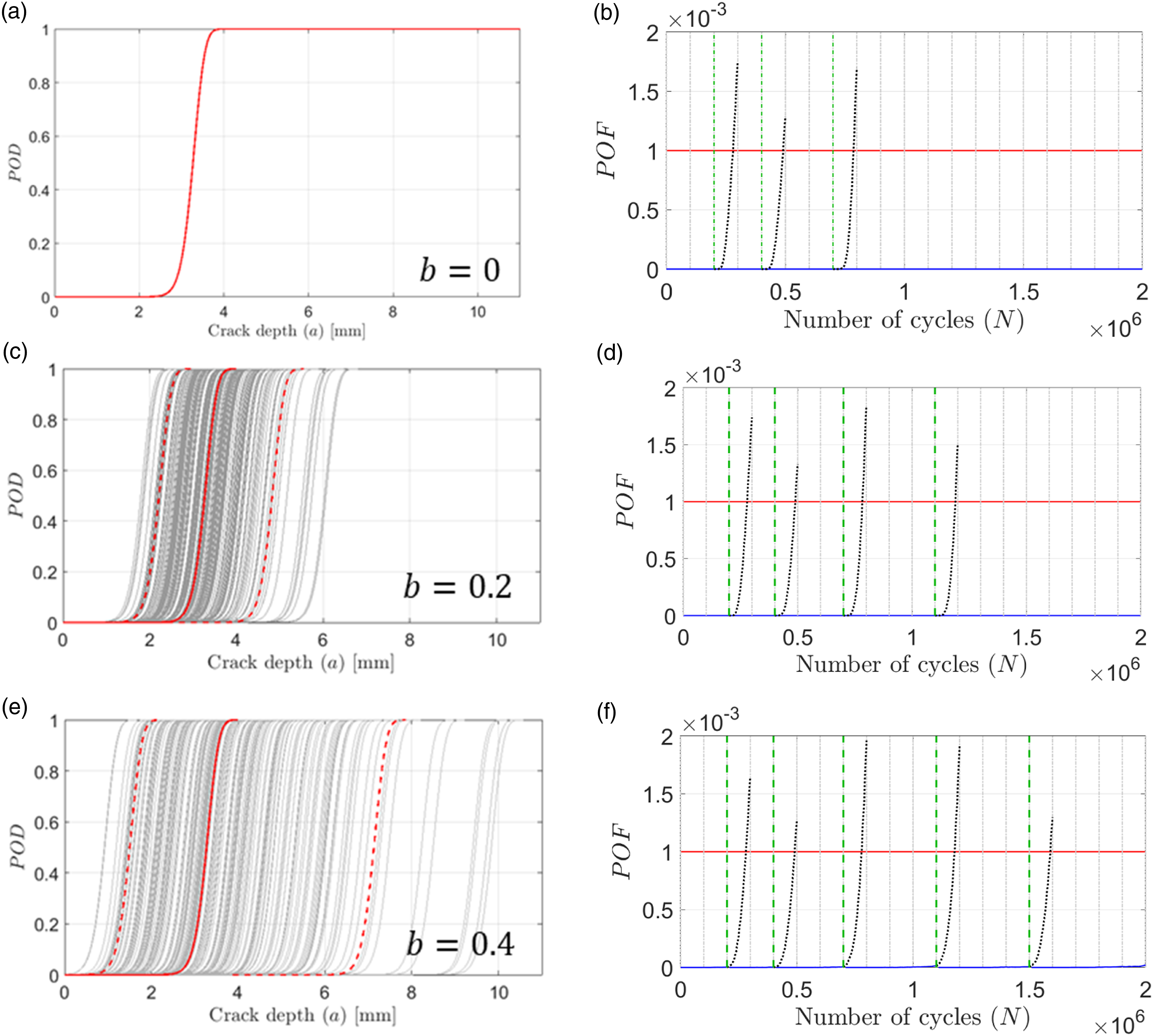
Various amount of systematic uncertainty in detection capabilities of permanently installed monitoring systems, represented as POD curves in (a), (c) and (e); the corresponding life-cycle management results, represented with the plot of projected remaining cycles until $PO F_{c r i t}$ against the number of cycles experienced by the component as shown in (b), (d) and (f).

This distribution of POD curves is applied to the example problem with various values of $b$ ( $b = 0$ , $0.2$ and $0.4$ ) to investigate the effect of varying degrees of systematic uncertainty. The curve for $b = 0$ and the expected (mean) curve is the same as the example monitoring system used previously in this study. The plots of the projected probability of failure against the number of loading cycles are shown in Figure 16(b), (d) and (f), respectively. The corresponding plots of POD curves are shown in Figure 16(a), (c) and (e). The grey plots in the figure are plots of selected POD curves sampled from the distribution, and the dotted red line are the 5% and 95% confidence bounds.

Figure 16 illustrates that as the confidence in the monitoring system is reduced, so too is the confidence in the integrity of the structure, resulting in the requirement of more manual inspections. With systematic uncertainty introduced, it becomes possible that a series of negative measurements is caused by an unfavourable combination of systematic effects hindering the detection capabilities of the monitoring system (e.g. defect being in an unfavourable location). To address the reduction in confidence in the monitoring system, more manual inspections need to be carried out to ensure the integrity of the component of interest.

Conversely, an increase in the confidence of the monitoring system leads to improved confidence in FFS. Clearly, the uncertainty in the detection capabilities defined here is arbitrary, but the results demonstrate the importance of taking into account the systematic uncertainties in the POD curves of the monitoring system. To be able to take advantage of frequent measurements from a monitoring system, there must be sufficient confidence in the detection capability of the monitoring system.

Discussion

The value of permanently installed monitoring systems becomes evident when their use in life-cycle management is quantified. The framework proposed in this article uses particle filtering methods to integrate damage detection data and probabilistic defect growth models for FFS analysis. With successive negative results from the monitoring system, the less probable defect growth paths are filtered based on the results, thus recursively updating the estimated FFS of the monitored component.

Using the successive negative results from permanently installed monitoring systems to filter the possibility of substantial damage can be a very effective way of maintaining confidence in the FFS of engineering components. Due to the stringent safety requirements of most engineering applications, the required probability of failure must be maintained at a very low level. The life of a component is usually limited by the remote chance that there is a severe defect. In such cases, monitoring is shown to be an effective tool as it facilitates the near-continuous screening for extreme cases providing assurance that failure is not imminent.

Due to the fixed position of permanently installed sensors, systematic uncertainty due to the relative positions of the sensor and the growing defect can result in poor confidence in the detection capabilities. It has been demonstrated that lack of confidence in the detection capability can severely undermine the estimated probability of failure as successive negative measurements may simply be a result of an inappropriate choice of sensor where area coverage is insufficient, or that the sensor has been poorly placed. It is therefore important to design a monitoring system with adequate area coverage to sufficiently cover all regions where defects may occur, such that the minimum detection capabilities are not too low, a concept which is explored in more detail in.²⁴

There is a well-known compromise between area coverage and sensitivity with permanently installed sensors. There is therefore a strong link between the confidence in defect location and the potential utility of permanently installed monitoring systems. The more confidence there is in defect location the more localised a monitoring system can be, which typically translates to greater sensitivity. Greater sensitivity means that the detection capabilities are improved which provides greater confidence in the fitness for service. If the detection capabilities of the monitoring system can reach a sufficient level, then the need for inspections can be completely eliminated.

The proposed approach simply treats the output of permanently installed monitoring systems as binary detection/no detection results similar to what is proposed in Reference 1 and 53; the key benefit being that the method can be used throughout the life of the component before any detectable damage is present. It is useful to consider the eventuality of a positive detection. Once a defect has been detected, its size can typically be estimated using the measurements from the monitoring system. The uncertainty quantified size estimate can then be used as the likelihood function to forecast failure time and FFS as schematically illustrated in Figure 17. Comparing this to the schematic illustration in Figure 2, the uncertainty in damage growth is considerably reduced as a growing defect has now been detected and sized. Successive measurements and sizing through monitoring or inspections would further reduce the uncertainty as to when the detected defect would reach the critical size. Methods of doing so has been the focus of previous literature on the use of particle filtering methods for FFS assessment and remnant life predictions.^21,40,54

Figure 17.

Schematic illustration of when a positive monitoring result is obtained, where sizing using the monitoring data can be done to perform more accurate remnant life predictions.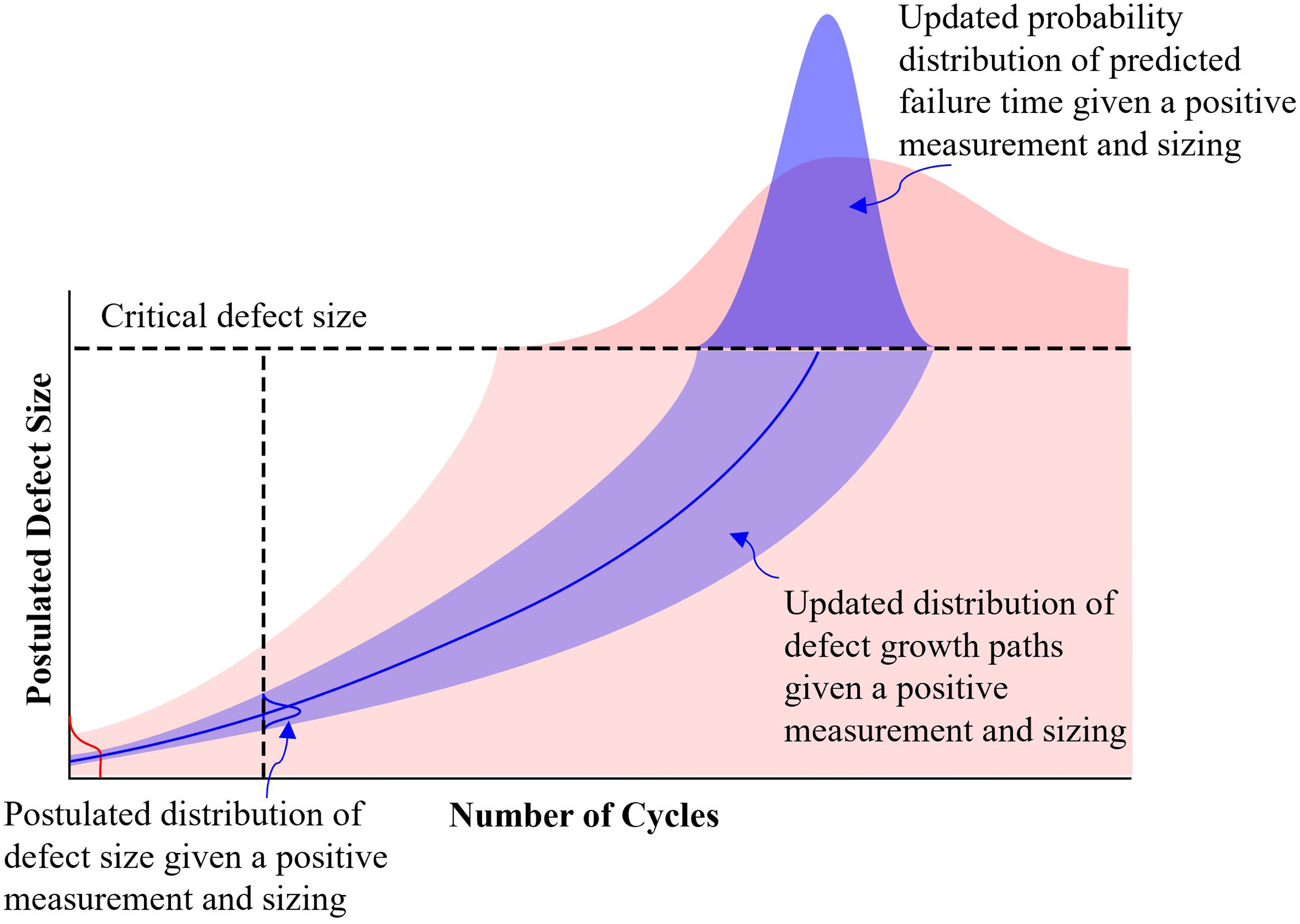

A hypothetical example problem was used in this article to demonstrate how the proposed framework can be applied to different problems. Despite simplifications in defect growth models and the choice of POD curves, the modularity of the proposed framework means that different defect growth models and POD models can be easily substituted as necessary for the specific problem. The only limitation to this proposed approach would be requirements in computational power and the amount of complexity in the models used.

Overall, the ability to take measurements near-continuously using permanently installed monitoring systems was shown to provide more confidence on the state of damage of the monitored component. This research demonstrated in particular how simply using a series of negative measurements can effectively filter the possibility of any substantial damage being present, thereby near-continuously updating our confidence in the FFS of the monitored component.

Conclusions

A framework that utilises detection data from permanently installed monitoring systems to estimate the FFS of engineering components is proposed. Using particle filtering methods, frequent measurements from permanently installed monitoring systems may be used to recursively update the distribution of postulated defect size, which in turn can be used to update the probability of failure.

A simulated example of a welded pipe undergoing three-point fatigue bending is used to demonstrate the value of the proposed framework. The hypothetical cases of managing the pipe using periodic inspections only or a combination of inspection and monitoring are evaluated. Results of the study show that the ability of permanently installed monitoring systems to filter cases of substantial damage is an effective way of maintaining confidence in fitness-for-service of engineering components. This translates to fewer in-service inspections required that may be costly and hazardous to conduct.

An implementation of the particle filtering method to incorporate the effect of systematic uncertainties in the detection capability of permanently installed monitoring systems is also proposed. By defining a distribution of POD curves, the effect of systematic uncertainties can be quantified and incorporated into the proposed particle filtering approach. Hypothetical distributions of POD curves were implemented into the example problem to demonstrate the importance of considering confidence in the detection capabilities of permanently installed monitoring systems and how the proposed method can take into account the effect of systematic uncertainties.

The effectiveness of using permanently installed monitoring systems is dependent on multiple factors such as the detection capabilities of the monitoring system, operating conditions, the failure criterion and the number of opportunities to inspect. It is proposed that the framework can be used to quantify the benefit of using permanently installed monitoring and promoting their adoption in suitable engineering applications.

Footnotes

Acknowledgements

The authors would also like to thank Prof. Peter Cawley and Prof. Michael Todd for their valuable guidance and support in this research.

Funding

The author(s) disclosed receipt of the following financial support for the research, authorship, and/or publication of this article: This work was supported by the UK Engineering and Physical Sciences Research Council via the UK Research Centre in NDE, grant EP/L022125/1.

ORCID iDs

Michael Siu Hey Leung

Joseph Corcoran

References

Medina

Aldrin

Knopp

, et al. Value assessment tools for hybrid NDE-SHM life management strategies. Mater Manuf Dir Air Force Res Lab 2006.

Mudge

Haig

Thornicroft

, et al. ‘Non-Invasive monitoring strategies for engineering structures using guided waves’. Presented at the 7th Middle East Nondestructive Testing Conference & Exhibition. Bahrain, 2015.

Cawley

. Structural health monitoring: Closing the gap between research and industrial deployment. Struct Health Monit 2018; 17: 1225–1244. DOI: 10.1177/1475921717750047.

Moslehi

Black

Faridian

. Multifunctional Fiber Bragg Grating sensing system for load monitoring of composite wings. In: Aerospace conference, Big Sky, MT, USA, 11 April 2011. USA, Big Sky: IEEE, 2011, pp. 1–9. DOI: 10.1109/AERO.2011.5747387.

Han

. Structural health monitoring of civil infrastructure using optical fiber sensing technology: a comprehensive review. Sci World J 2014; 2014: 1–11. DOI: 10.1155/2014/652329.

Pöckl

Kleinöder

. Developing and Implementation of a Fatigue Monitoring System for the New European Pressurized Water Reactor EPR. Germany: AREVA NP GmbH, 2007.

Nayeri

Masri

Ghanem

, et al. A novel approach for the structural identification and monitoring of a full-scale 17-story building based on ambient vibration measurements. Smart Mater Struct 2008; 17(2): 025006.

Pizhong Qiao

Qiao

. Vibration-based Damage Identification Methods: A Review and Comparative Study. Struct Health Monit 2011; 10(1): 83–111. DOI: 10.1177/1475921710365419.

Holford

Pullin

Evans

, et al. Acoustic emission for monitoring aircraft structures. Proc Inst Mech Eng G: J Aerospace Eng 2009; 223(5): 525–532.

10.

Sengupta

Datta

Topdar

. Structural damage localisation by acoustic emission technique: A state of the art review. Latin Am J Sol Struct 2015; 12(8): 1565–1582. DOI: 10.1590/1679-78251722.

11.

Orcesi

Frangopol

. Optimization of bridge maintenance strategies based on structural health monitoring information. Struct Saf 2011; 33(1): 26–41.

12.

Thöns

Schneider

Faber

. Quantification of the Value of Structural Health Monitoring Information for Fatigue Deteriorating Structural Systems. Canada: SHM, 2015.

13.

Colombo

. Applications of Structural Health Monitoring and Field Testing Techniques to Probabilistic Based Life-Cycle Evaluation of Reinforced Concrete Bridges. São Paulo: Doutorado em Engenharia de Estruturas, Universidade de São Paulo, 2016. DOI: 10.11606/T.3.2016.tde-02122016-092514.

14.

Mondoro

Soliman

Frangopol

. Prediction of structural response of naval vessels based on available structural health monitoring data. Ocean Eng 2016; 125: 295–307. DOI: 10.1016/j.oceaneng.2016.08.012.

15.

Loveday

Long

. Long range guided wave defect monitoring in rail track. AIP Conf Proc 2014; 1581(1): 179. DOI: 10.1063/1.4864818.

16.

Yanan

Changzheng

. Acoustic emission detection of fatigue cracks in wind turbine blades based on blind deconvolution separation. Fatigue Fracture Eng Mater Struct 2016; 40(6): 959–970. DOI: 10.1111/ffe.12556.

17.

Jiao

Cheng

, et al. Monitoring fatigue cracks of a metal structure using an eddy current sensor. EURASIP J Wireless Commun Networking 2016; 2016: 188. DOI: 10.1186/s13638-016-0689-y.

18.

Chua

Cawley

. Crack growth monitoring using fundamental shear horizontal guided waves. Struct Health Monit 2020; 19: 1311–1322. DOI: 10.1177/1475921719882330.

19.

Ling

Mahadevan

. Integration of structural health monitoring and fatigue damage prognosis. Mech Syst Signal Process 2012; 28: 89–104. DOI: 10.1016/j.ymssp.2011.10.001.

20.

Leung

MSH

Corcoran

Cawley

, et al. Evaluating the use of rate-based monitoring for improved fatigue remnant life predictions. Int J Fatigue 2019; 120: 162–174. DOI: 10.1016/j.ijfatigue.2018.11.012.

21.

Corbetta

Sbarufatti

Giglio

, et al. Optimization of nonlinear, non-Gaussian Bayesian filtering for diagnosis and prognosis of monotonic degradation processes. Mech Syst Signal Process 2018; 104: 305–322. DOI: 10.1016/j.ymssp.2017.11.012.

22.

Sikorska

Hodkiewicz

. Prognostic modelling options for remaining useful life estimation by industry. Mech Syst Signal Process 2011; 25(5): 1803–1836. DOI: 10.1016/j.ymssp.2010.11.018.

23.

Sun

Zuo

Wang

, et al. Prognostics uncertainty reduction by fusing on-line monitoring data based on a state-space-based degradation model. Mech Syst Signal Process 2014; 45(2): 396–407. DOI: 10.1016/j.ymssp.2013.08.022.

24.

Leung

MSH

. Probabilistic Approach to Structural Integrity Assessment of Fatigue Damage Using Permanently Installed Monitoring Systems, PhD Thesis. London, UK: Imperial College, 2020.

25.

Guide to Methods for Assessing the Acceptability of Flaws in Metallic Structures, British Standards Institution, BS 7910 2019. Accessed: 09 January 2020. [Online]. Available: https://bsol.bsigroup.com/Bibliographic/BibliographicInfoData/000000000030369478.

26.

Shibata

Takeyama

. Pitting corrosion as a stochastic process. Nature 1976; 260(5549): 315–316. DOI: 10.1038/260315a0.

27.

Virkler

Hillberry

Goel

. The statistical nature of fatigue crack propagation. J Eng Mater Tech 1979; 101(2): 148–153. DOI: 10.1115/1.3443666.

28.

Roy

Ghosh

Bose

. A stochastic model for evolution of creep damage in engineering materials. Trans Indian Inst Met 2010; 63(2): 665–669. DOI: 10.1007/s12666-010-0101-2.

29.

Appalanaidu

Vyas

Gupta

. Stochastic creep damage growth due to random thermal fluctuations using continuum damage mechanics. Proced Eng 2013; 55: 805–811. DOI: 10.1016/j.proeng.2013.03.335.

30.

Gobbato

Conte

Kosmatka

. Statistical performance assessment of an NDE-Based SHM-DP methodology for the remaining fatigue life prediction of monitored structural components and systems. Proc IEEE 2016; 104(8): 1575–1588. DOI: 10.1109/JPROC.2015.2512979.

31.

Probabilistic Methods for Planning of Inspection for Fatigue Cracks in Offshore Structures, DNVGL, Recommended Practice RP-C210, 2015.

32.

Miedlar

. Summary of stress intensity factor information. In: AFGROW Handbook for Damage Tolerant Design. AFGROW, 2002.

33.

Elber

. Equivalent constant-amplitude concept for crack growth under spectrum loading. In: Wei

Stephens

(eds). Fatigue Crack Growth Under Spectrum Loads. West Conshohocken, PA: ASTM International; 1976, pp. 236. DOI: 10.1520/STP33376S.

34.

Lan

. Traffic load modelling based on structural health monitoring data. Struct Infrastruct Eng 2011; 7(5): 379–386. DOI: 10.1080/15732470902726809.

35.

Jouan

Bergholz

Rudolph

. Fatigue monitoring approaches for power plants. In: Codes and Standards, Vol 1. California, USA: Anaheim, 2014, p. V001T01A035. DOI: 10.1115/PVP2014-28100.

36.

Mohseni

Habibzadeh Boukani

Ramos França

, et al. A study of the automated eddy current detection of cracks in steel plates. J Nondestr Eval 2020; 39(1): 6. DOI: 10.1007/s10921-019-0647-9.

37.

Chua

Cawley

Nagy

. Scattering of the fundamental shear guided wave from a surface-breaking crack in plate-like structures. IEEE Trans Ultrason Ferroelectr, Freq Control 2019; 66: 1887–1897. DOI: 10.1109/TUFFC.2019.2932227.

38.

Herdovics

Cegla

. Long-term stability of guided wave electromagnetic acoustic transducer systems. Struct Health Monit 2018; 19(1): 3–11. DOI: 10.1177/1475921718805733.

39.

Arulampalam

Maskell

Gordon

, et al. A tutorial on particle filters for online nonlinear/non-Gaussian Bayesian tracking. IEEE Trans Signal Process 2002; 50(2): 174–188. DOI: 10.1109/78.978374.

40.

Cadini

Zio

Avram

. Monte Carlo-based filtering for fatigue crack growth estimation. Probab Eng Mech 2009; 24(3): 367–373. DOI: 10.1016/j.probengmech.2008.10.002.

41.

Karve

Guo

Kapusuzoglu

, et al. Digital twin approach for damage-tolerant mission planning under uncertainty. Eng Fract Mech 2020; 225: 106766. DOI: 10.1016/j.engfracmech.2019.106766.

42.

Johnson

. The history, logic and uses of the Equivalent Initial Flaw Size approach to total fatigue life prediction. Proced Eng 2010; 2(1): 47–58. DOI: 10.1016/j.proeng.2010.03.005.

43.

Koçak

. European Fitness for Service Network: Final Technical Report, GTC-2001-43049. 2007.

44.

McKay

Beckman

Conover

. Comparison of three methods for selecting values of input variables in the analysis of output from a computer code. Technometrics 1979; 21(2): 239–245. DOI: 10.2307/1268522.

45.

Kozierski

Lis

Zietkiewicz

. Resampling in Particle Filtering - Comparison. Poznań Society of Friends of Learning, 2013.

46.

Bolic

Djuric

. Resampling methods for particle filtering: classification, implementation, and strategies. IEEE Signal Process. Mag 2015; 32(3): 70–86. DOI: 10.1109/MSP.2014.2330626.

47.

Sattar

Sun

. Deterministic resampling: unbiased sampling to avoid sample impoverishment in particle filters. Signal Process. 2012; 92(7): 1637–1645. DOI: 10.1016/j.sigpro.2011.12.019.

48.

Schubert Kabban

Greenwell

DeSimio

, et al. The probability of detection for structural health monitoring systems: Repeated measures data. Struct Health Monit 2015; 14: 252–264.

49.

Leung

MSH

Corcoran

Cawley

. ‘A Structural Integrity Informed Approach to Evaluating the Probability of Detection Obtained with Permanently-Installed Sensors’, Presented at the 46th Annual Review of Progress in Quantitative Nondestructive Evaluation. Portland: OR, 2019.

50.

Haslinger

Lowe

MJS

Huthwaite

, et al. Elastic shear wave scattering by randomly rough surfaces. J Mech Phys Sol 2020; 137: 103852. DOI: 10.1016/j.jmps.2019.103852.

51.

Gajdacsi

. High Accuracy Ultrasonic Degradation Monitoring. PhD Thesis, 2015.

52.

Foucher

Fernandez

Leberre

, et al. New Tools in CIVA for Model Assisted Probability of Detection (MAPOD) to Support NDE Reliability Studies. Bridgeton, 2018.

53.

Stutzmann

Ziegler

Muskulus

. Fatigue crack detection for lifetime extension of monopile-based offshore wind turbines. Energ Proced 2017; 137: 143–151. DOI: 10.1016/j.egypro.2017.10.341.

54.

Chen

Yuan

Wang

, et al. On particle filter improvements for on-line crack growth prognosis with guided wave monitoring. Smart Mater Struct 2019; 28(3): 035011. DOI: 10.1088/1361-665X/aaf93e.

A probabilistic method for structural integrity assurance based on damage detection structural health monitoring data

Abstract

Introduction

Description of example problem

Description of the structural problem and damage growth model

Description of the inspection and monitoring schemes

Eddy current sensor for inspection

Guided wave sensor for monitoring

Method

Bayesian inference for a single measurement result

Particle filtering for repeated measurements

Forecasting estimated probability of failure

Inspection decision and updating

Results for the example problem

Integrity assessment with inspections only

Integrity assessment with inspections and monitoring

The effect of systematic uncertainty in the detection capability of permanently installed monitoring systems

Particle filtering incorporating uncertainty in POD curve

Results incorporating uncertainty in POD curve

Discussion

Conclusions

Footnotes

Acknowledgements

Funding

ORCID iDs

References