Sage Journals: Discover world-class research

Abstract

In recent years, electrical tomography, namely, electrical resistance tomography (ERT), has emerged as a viable approach to detecting, localizing and reconstructing structural cracking patterns in concrete structures. High-fidelity ERT reconstructions, however, often require computationally expensive optimization regimes and complex constraining and regularization schemes, which impedes pragmatic implementation in Structural Health Monitoring frameworks. To address this challenge, this article proposes the use of predictive deep neural networks to directly and rapidly solve an analogous ERT inverse problem. Specifically, the use of cross-entropy loss is used in optimizing networks forming a nonlinear mapping from ERT voltage measurements to binary probabilistic spatial crack distributions (cracked/not cracked). In this effort, artificial neural networks and convolutional neural networks are first trained using simulated electrical data. Following, the feasibility of the predictive networks is tested and affirmed using experimental and simulated data considering flexural and shear cracking patterns observed from reinforced concrete elements.

Keywords

Artificial intelligence deep learning electrical resistance tomography inverse problems neural networks structural health monitoring

Introduction

Background

Structural health monitoring (SHM), in a broad sense, aims to assess the integrity, condition and/or damage state of target structures.¹ Respectively, SHM frameworks have proposed clear hierarchies including, for example, aspects such as detection, localization, classification, assessment, and prediction which serve as facets for monitoring.² For such hierarchies to be satisfied, SHM modalities should therefore include systematic, automatic and continuous data acquisition followed by accurate post-processing and analysis. To address the latter needs, specifically rapid and accurate damage assessment of structural concrete elements, this work focuses on rapid probabilistic crack prediction and localization enabled by machine learned models.

Prediction and localization of cracking in concrete elements is well documented in the field of non-destructive testing (NDT) literature. Various traditional approaches include ultrasonic, magnetic, electromagnetic, radiographic, photographic, and infrared modalities.^3–7 In contrast to these well-established methods, electrical-based modalities have recently shown promise in non-destructive testing and evaluation of cement-based materials and structures.⁸ For example, in their seminal work, Karhunen et al.⁹ demonstrated industrial applicability of electrical modalities for assessing the degree of cracking, localization of reinforcement, corrosion state and depth of the cover in concrete elements. Additionally, previous studies have shown that electric impedance spectroscopy (EIS) is relatively inexpensive and can be applied on concrete elements to detect cracks to include their width/depth, reinforcement and internal moisture.^10,11 On the other hand, electrical tomography, more specifically electrical resistance tomography (ERT, a specific electrical tomography modality), has been recently demonstrated as an effective modality for detecting simple and complex cracking patterns in concrete elements ^9,12–14; meanwhile, ERT has low experimental costs, energy consumption, fast data collection, high temporal resolution and potential of continuous spatial monitoring.¹⁵ However, the potential disadvantages of ERT include its lower spatial resolution compared with other contemporary modalities and (traditionally) high computational cost.¹⁶

In assessing the former realizations regarding ERT, relatively low spatial resolution may be sufficient in terms of localizing cracks – especially in large members.¹⁷ Furthermore, the high computational cost that traditionally arises in ERT stems from solving the ill-posed inverse problem. Though previous research has demonstrated that incorporating non-iterative reconstruction methods can reduce the computational time at a significant cost to spatial resolution (often overly smooth), computational demand and interpretability of reconstructions remain factors inhibiting implementation of ERT in field applications. As such, a new methodology promoting rapid and accurate cracking prediction from ERT data sets is needed. To address this issue, the following article proposes and investigates the implementation of neural networks (NNs) to directly solve an analogous ERT inverse problem affording (a) massive reduction in computing demand and prediction time relative to high-fidelity ERT reconstruction frameworks and (b) improved interpretability of (predicted) cracking patterns.

Machine learning and damage prediction

The concept of using NNs for pattern recognition and parameter space mapping originated in mid-20th century ¹⁸ and has drawn large research interest since the discovery of back-propagation while computational power has been increasing exponentially. In fact, previous studies have indicated that a well-trained network with two neurons is sufficient to recognize any linear functions between the input and output data sets theoretically.¹⁹ However, realistically, a deeper network with nonlinear activation functions is required to predict more complex representations.¹⁹ For this reason, we investigate the use of supervised deep learned NNs for mapping input data to desired output parameters, as detailed in the following.

Feed-forward artificial neural networks (ANNs) have architectures consisting of at least one hidden and one output layer. In a pioneering work, Baum ²⁰ proved that a simple one-layer network can recognize a linear pattern. Following, work by Papert et al. ¹⁹ discovered that an ANN network with N − 1 neurons should be sufficient to learn an arbitrary function with N data points. Subsequent early research also indicated that networks having M ≪ N − 1 weights have approximately 50% probability of successfully predicting a random function.²¹ Later, Lecun et al.²² identified that a well-trained binary classifier is capable of linearly separating the error space by a hyper-plane. This enabling feature is key in the ability of NNs to recognize highly nonlinear patterns. However, despite tremendous research progress in ANN research, tailoring ANN parameterizations still remains an ‘art’ in practice.

In contrast to ANNs, convolutional neural networks (CNNs) are NN architectures first trained with back-propagation by Lecun et al. and inspired by human ventral visual stream.^23,24 Convolutional neural networks are widely used for handwriting, image, and voice classification – along with other recognition applications.²⁵ A typical CNN’s functionality depends on four basic layers which are input layer, convolutional layer, pooling layer and fully connected layer.²⁶ Firstly, in the input layer, CNNs take input information via an image matrix where (broadly speaking) each entry is either a continuous entry or assigned a whole number varying from 0 to 255 representing the scale of each pixel from black to white. Secondly, within the convolutional layers, learnable kernels are glided through the raw input while the scalar products are calculated for each entry in the kernels; the output of this convolution operation is referred as feature maps. Each kernel has its corresponding feature map which is stacked along the depth of the input.²⁷ Kernels can help the network to extract more characteristic information from input data.²⁶ The convolution operation is mainly governed by the following three hyperparameters: 1. depth of the convolutional layer, 2. stride of the kernels and 3. padding.²⁸ Reducing the depth of the convolutional layers can lead to a significant decrease in network’s recognition capability. Meanwhile, stride controls the overlap when kernels are glided through the input data, by reducing the stride, one can reduce the output volumes however at the risk of missing potential features. In addition, the use of zero padding ensures that features at the extents of the image input can be efficiently extracted. Furthermore, parameter sharing can be used to reduce the number of parameters in the network by constraining the learned feature maps to have the same weight and bias.²⁶ Thirdly, a pooling layer aims to further downsample convolved data. For example, a max pooling layer is applied on the feature maps and only returns the maximum value within the region. Finally, data are propagated to a fully connected layer which has a similar structure to a typical ANN. Of importance here, the inputs of the (first) fully connected layer are the outputs of the last pooling layer which are subsequently propagated through the remaining fully connected layers during the training.²⁷

Specifically, we are interested in direct classification of spatially distributed damage (cracking) which is assigned a binary form (0 or 1). As such, the use of probabilistic cross-entropy classification is most appropriate given the binary nature of the information to be mapped (i.e. classical regression is not appropriate). Therefore, we select the binary cross-entropy function as the loss functional to be minimized in the network training, written as follows

ℒ = - \frac{1}{N} \sum_{t = 1}^{N} [y_{t} \log (p_{t}) + (1 - y_{t}) \log (1 - p_{t})]

(1)

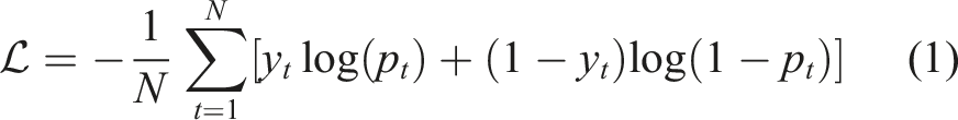
In equation (1), $ℒ$ represents the binary cross-entropy loss taking predictions p_t and binary sample labels y_t across t ∈ N training samples.²⁹ The interpretation of minimizing equation (1), in the learning process, may be viewed as gradually improving the probability $P$ that predictions p_t match the true distributions y_t. As it pertains to this work, this corresponds to learning the underlying patterns governing the predictions of cracks where, using relaxed notation, $P = 1$ and $P = 0$ , respectively, correspond to cracked and not cracked locally. Pragmatically speaking, however, minimizing equation (1) may lead to over fitting and reduced generalizability. Therefore, L₂ regularization is herein utilized to address the former by writing

ℒ = - \frac{1}{N} \sum_{t = 1}^{N} [y_{t} \log (p_{t}) + (1 - y_{t}) \log (1 - p_{t})] + λ {‖ w ‖}^{2}

(2)

where λ is a scalar regularization hyperparameter and w are the network weights.

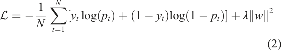
Generally speaking (and herein), equation (2) is minimized by implementing gradient decent and back-propagation via locating the minimum point within the loss space. It is worth noting that, despite developments of, for example, the Hopfield network and Boltzmann machine which offer new insight of training networks with statistical mechanics,^30,31 many modern networks still rely on gradient decent and back-propagation. Moreover, while local minima can be reached by adjusting the weights of individual neurons in the network iteratively, there exist studies indicating a global minimum could be attained providing a deep neural network with non-convex objective function,³² although the evidence supporting that is not substantial. Therefore, for the purposes of this initial work, a local minimum can be assumed to yield results deemed sufficient for the purposes of damage detection.

It is worth highlighting that, in the context of contemporary SHM research, machine learning has been successfully used in damage detection applications. For example, Bao et al.³³ utilized neural networks for optimization considering non-convex sparse time–frequency analysis and consequently achieved more accurate instantaneous frequency identification. Moreover, Mousavi et al.³⁴ trained deep neural networks to extract damage-sensitive features from vibration data. In addition, convolutional neural networks were also explored to retrieve missing strain data due to sensor fault by Oh et al.³⁵ while Mohtasham used CNNs to detect cracks on gas turbines with filtered image data.³⁶ Inspired by such works, in this article, neural networks are also utilized for the intended purposes of SHM.

Article structure

This article first reviews the historical development and application of ERT as well as a conventional solution to the ill-posed ERT problem. Then, the deep learned direct inversion framework is proposed. Thereafter, the data acquisition and training methodology consisting of the training data generation, neural network architecture as well as the training process are detailed. Following, predictive results for experimental and simulated crack patterns are reported and discussed considering both their advantages and drawbacks. Lastly, conclusions are provided.

Electrical resistance tomography and direct inversion

Electrical resistance tomography is a modality which aims to reconstruct internal conductivity distributions from boundary electrode measurement. To achieve this, a prescribed number of electrodes are installed on the boundary of the specimen, from which electrode potentials are measured and electric currents are injected into. Resultingly, potential differences are taken between one pair of electrodes for each injection. As a whole, the measurement protocol should be planned in a systematic manner to ensure sufficient data can be collected during each injection.

Historically speaking, ERT was initially developed and utilized for medical imaging by classifying organs based on their different conductivities,³⁷ later considering capacitive and inductive tomographies.³⁸ In the recent years, ERT has been the source of significant research interest in the NDT/SHM community. For this, ERT has been coupled with sensing skins to detect damage in reinforced concrete ^13,39,40 as well as imaging damage, strain and stress fields in a broad suite of composite materials.^41–48 Previous related studies also demonstrate that ERT is capable of imaging internal moisture flow within cement-based material in both 2D and 3D settings.^8,49

Until recently, high-fidelity solutions to the ERT reconstruction problem have generally required solving an optimization problem using conventional iterative regularized computational methods (readers are referred to ¹⁶ for a comprehensive review of ERT inversion methods used in NDT). However, as earlier alluded to, such methods can be demanding and pragmatically inhibiting. On the other hand, linearized difference imaging schemes offer much faster solutions at the cost of spatial resolution.⁵⁰ As such, we herein take a different approach to the ERT inversion problem by utilizing direct inversion enabled by trained NNs in order to attain rapid high-fidelity predictions. Related work has, for example, aimed at using NNs for solving the continuous ERT problem.⁵¹ Additional research has shown that CNNs are capable of reconstructing ERT image data ^52,53 however not for detecting cracking in structural applications. Recently, researchers in Reference 54 also used NNs to optimize the electrode locations in ERT measurement aiming at achieving more efficient data acquisition. In the following section, written for contextualization, we will first discuss the forward problem underlying ERT physics (and used for generating training data), then discuss the conventional ERT inverse problem and finally propose the analogous ERT direct inversion framework.

The ERT forward model

In order to reconstruct the internal conductivity distribution, an ill-posed ERT inverse problem needs to be solved. The ill-posed nature of this problem results from a number of factors, including (a) ill-conditioning of matrices used in the optimization, (b) experimental measurement noise and (c) the diffusive nature of electric fields.² Nonetheless, in order to implement ERT computationally, a numerical forward model is required in order to map the internal conductivity to boundary measurements. For this, we utilize the complete electrode model (CEM), which is implemented using finite elements^55,56 discretizing the following equations

\nabla \cdot (σ \nabla u) = 0, x \in Ω

(3)

\int_{e_{l}} σ \frac{\partial u}{\partial n} d S = I_{l}, l = 1, \dots ., L

(4)

σ \frac{\partial u}{\partial n} = 0, x \in \partial Ω / \cup_{l = 1}^{L} e_{l}

(5)

u + z_{l} σ \frac{\partial u}{\partial n} = U_{l}, l = 1, \dots ., L

(6)

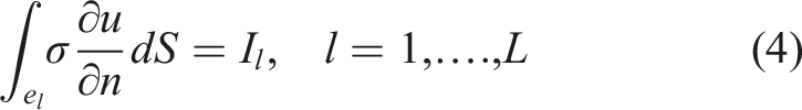
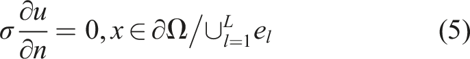
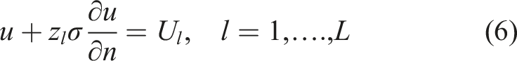
Equation (3) is the Laplace equation which describes steady-state diffusion⁴⁷ in a target domain Ω with a boundary ∂Ω. Further, x represents Cartesian coordinates within the domain while σ(x) and u(x) represents the conductivity distribution and potential distribution within the target. Equations (4)–(6) provide the necessary boundary conditions to solve equation (3), where e_l represents the l^th electrode; hence, U_l is the potential measurement on the corresponding electrode. I_l represents the current injection on l^th electrode. dS represents the infinitesimal surface of Ω while z_l represents the contact impedance between the l^th electrode and the internal domain. Equations (4)–(6) provide an accurate forward model solution by taking the shunting effects of electrodes and their contact impedance into account.⁵⁷ Lastly, in order to satisfy the current conservation law and fixed potential reference level which would ensure an unique solution, the following equations are written to complete the CEM

\sum_{l = 1}^{L} I_{l} = 0

(7)

\sum_{l = 1}^{L} U_{l} = 0

(8)

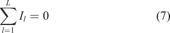
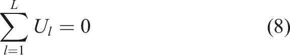
We would like to emphasize that the CEM describes the forward problem where the internal conductivity is known, from which the electrode potentials can be computed. As such, we adopt the CEM in generating training data sets which consist of boundary voltage measurements accompanied by corresponding internal conductivity distribution is known. However, in pragmatic imaging scenarios, the internal conductivity distribution is unknown. Therefore, conductivity estimates must be obtained using an inverse methodology as described in the forthcoming sections.

The ERT inverse problem

The traditional nonlinear ERT inverse problem can be conceptually characterized by the following observation model

V = U (σ)

(9)

where U is the finite element forward model mapping σ to measured voltages V. Such a model implies that when the measurements and the forward model match exactly, the inverse problem is solved (i.e. when the L₂ norm of the data fidelity term is minimized: ‖V − U(σ)‖² = 0). In reality, however, such a case is an unrealistic idealization as measurement noise e is always present, resulting in the noise-modified observation model written as

V = U (σ) + e

(10)

Unfortunately, due to the presence of noise, numerical modelling error, nonlinearity of U(σ), and ill-conditioning of resulting ERT matrices used in solving the inverse optimization problem, there are infinite solutions to equation (10). Thus, we require advanced regularization to incorporate biasing prior information and, often, physical constraints in optimizing/solving the nonlinear (absolute imaging) inverse problem. In order to avoid such complexities, the observation model may be linearized in order to obtain solutions with less up-front computational demand/complexity.⁵⁸

Linearized ERT, or simply difference imaging as we will herein refer to it, is a framework which aims to reconstruct the difference of internal conductivity Δσ based on differences of boundary voltage measurements ΔV from two different states (subscripts 1 and 2 representing baseline and damaged states, respectively) expressed in the following

Δ V = V_{2} - V_{1}

(11)

Δ σ = σ_{2} - σ_{1}

(12)

As a consequence, the following linearized observation model can be written

Δ V = J Δ σ + Δ e

(13)

where

J = \partial U (σ_{1}) / \partial σ_{1}

is the Jacobian matrix computed at the linearization point σ₁ and Δe is the difference in measurement noise between states 1 and 2.

Based on the observation model in equation (13), the ERT reconstruction problem is generally facilitated by a one-step least squares solution minimizing the following objective function

Ψ = {‖ L_{Δ e} (Δ V - J Δ σ) ‖}^{2} + α {‖ L_{R} Δ σ ‖}^{2}

(14)

where L_Δe and L_R are Cholesky factorized noise weighting and regularization matrices, respectively. The use of regularization, the magnitude of which is largely controlled by the hyperparameter α > 0, is required to stabilize solutions and incorporate prior information into the least squares minimizer described below

Δ \hat{σ} = {(J^{T} W J + α L_{R}^{T} L_{R})}^{- 1} J^{T} W Δ V

(15)

where W is a diagonal noise weighting matrix.

The advantages in adopting linearized schemes, such as the difference imaging approach described previously, are numerous. Firstly, since one-step optimization is used, inverse solutions are significantly less computationally demanding than nonlinear absolute imaging solutions. Secondly, and of principle importance to this work, the use of difference data ΔV results in subtraction of systematic errors. Therefore, in cases where measurements are simulated for use in training data, a significant portion of modelling errors are subtracted – thereby reducing the influence of modelling error corruption in training. In the following subsection, we will detail the incorporation of difference data into the learned direct inversion scheme analogous to the traditional linearized scheme previously described.

Analogous ERT direct inversion framework

This section introduces the learned framework used to directly solve the analogous ERT (crack reconstruction) inverse problem. Following, we provide rationale for the ANN and CNN architecture selections and learning approaches used in direct inversion.

Analogous ERT direct inversion approach

The overarching aim of the proposed direct inversion approach is to map ERT difference measurements ΔV to probabilistic binary crack distributions. The purpose for choosing a binary cracking representation is to simplify the interpretability of damage predictions. More technically, we aim to predict the probability of local cracking p_σ ∈ [0, 1], where a predicted value of 1 indicates that a pixel contains a crack with 100% predicted confidence. Conversely, a predicted value of 0 refers to 0% confidence of a crack within the pixel while intermediate predicted values convey uncertainty in the local occurrence of cracking. Summarily, we aim to learn the following mapping

A (Δ V) \to p_{σ}

(16)

where

A

is a symbolic functional representation of the learned network.

The function $A$ , while roughly analogous to the linearized difference imaging scheme with respect to ΔV, is highly nonlinear. This realization stems from the fact that the mapping between data ΔV and binary crack distributions results from (a) the nonlinear transformation of the parameterizations given by σ ∈ (0, + ] → p_σ ∈ [0, 1] and (b) the fundamentally nonlinear relationship between ERT measurements and conductivity (as the linearization assumption in conductivity is not made in learned direct inversion). Therefore, given the nonlinear relation between network inputs and outputs coupled with the idealized binary nature of p_σ, the use of linear and regressive networks might not be the most appropriate option for this work. Regarding the latter, this choice is justified because (a) we are aiming at reconstruct crack patterns in a binary manner which is categorized as a classification problem and (b) the distribution of binary data is inappropriate for regression. Hence, necessitating the use of deep networks optimized following equation (2). In the following section, we will describe the training and learning process for predictive networks $A$ .

Selection of machine learning architectures and learning approach for cracking classification

In this section, we introduce the potential algorithm options for solving a classification problem and justifications for our ANN and CNN selections. A significant analysis and discussion on classification techniques by Kotsiantis and coauthors⁵⁹ show that there are options as following: 1. logic based algorithms such as decision trees, 2. perceptron-based techniques such as single layered perceptrons and deep neural networks, 3. statistical learning algorithms such as Naive Bayes classifiers (NB) and Bayesian networks (BNs), 4. instance-based learning such as k-nearest neighbour (kNN) and 5. support vector machines (SVMs). Generally speaking, SVMs and neural networks yield more accurate outputs with multi-dimension input features. A quantitative study by Osisanwo et al.⁶⁰ shows that SVMs and NNs have better accuracy when tested with larger data sets and more attributes. However, SVMs are designed to be binary algorithms, and as a result, this feature can potentially limit its applications when dealing with non-binary classification problems. In addition, logic based algorithms are highly interpretable; however, the accuracy of such algorithms are significantly affected by the input features which need to be discretized in exchange for a higher classification accuracy.⁶¹ Furthermore, NNs have been found to be more reliable in providing incremental learning compared to decision trees.⁶² For statistical learning algorithms, although most of them require less computational time when compared to NNs, the assumption of independence between nodes has been shown to result in comparatively lower accuracy.⁵⁹ As a result, BN classifiers need large networks to reach high accuracy which is often not feasible; therefore, these algorithms may not be suitable when using large feature data sets.⁶³ For instance-based learning such as kNN, the choosing of k is essential especially when noise is present in the training input sets. However, currently there is a dearth in rigorous selection approaches for choosing k in pragmatic applications, thereby leading to large computational time for classifications.⁶⁴ Taken together, the above analysis suggests that NNs are the most suitable selection for this work, owing to their overall accuracy when solving classification problems having large feature inputs. Additionally, from a practical standpoint, NNs (a) have the ability to train using (input) data in the absence of prior knowledge on their distribution⁶⁵ and (b) without specifying an optimized mathematical model.⁶⁶

To further examine the performance of different neural networks for classification problems, Jeatrakul compared the performance between back-propagation neural network (BPNN), general regression neural network (GRNN), radial basis function neural network (RBNN), probabilistic neural network (PNN) and complementary neural network (CMTNN). Each network was tested against three benchmark data sets; in their work, the BPNN turned out to be the most robust across all three training tasks.⁶⁷ Furthermore, Pasupa and Sunshem compared a CNN with an ANN using smaller data sets showing that a CNN with regularization and dropout can provide comparable results to ANN,⁶⁸ thus supporting the selection of CNN classifiers for the purposes of this work.

Summarily, the studies reviewed in this subsection suggest that ANN and CNN architectures are suitable for the crack classification tasks investigated herein. Therefore, these two neural networks are adopted for the analogous ERT direct inversion framework, namely, the mapping of input data ΔV to the probability of local cracking p_σ.

Training data acquisition and training methodology

Overview

Training data were generated using the CEM equipped with quadratic triangular discretizations. A set of training samples herein consists of simulated electrode potential differences generated using sampled conductivity distributions and complimentary binary crack distributions described in the previous subsection. Regarding the potential measurements more specifically, each simulated difference measurement set results from subtracting baseline (undamaged) ERT measurements V₁ from ERT measurements V₂ generated from a cracked configuration.

In this work, two cracking phenomena are studied: flexure-induced cracking and shear-induced cracking. In total, 40,000 sets of training samples were generated for both flexural and shear cracks configurations. For validation purposes, geometries of the domains where flexural and shear cracks developed were chosen considering differing geometries. Domain geometry and experimental data for flexural cracking were adapted from the experimental ERT study¹³ while the domain geometry for shear crack was adapted from Reference 7. However, since raw ERT experimental data were not obtained during the shear testing, the shear cracking investigation uses simulated data generated from randomized shear crack distributions. Parameters of the domains that are developing both types of cracking are provided in Tables 1 and 2. We note that the use of simulated data also facilitates quantitative assessment with respect to true cracking patterns.

Table 1.

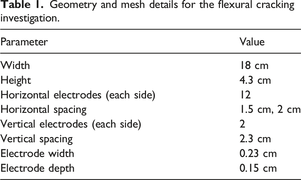
Geometry and mesh details for the flexural cracking investigation.

Parameter	Value
Width	18 cm
Height	4.3 cm
Horizontal electrodes (each side)	12
Horizontal spacing	1.5 cm, 2 cm
Vertical electrodes (each side)	2
Vertical spacing	2.3 cm
Electrode width	0.23 cm
Electrode depth	0.15 cm

Table 2.

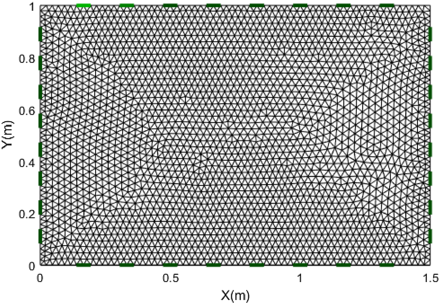
Geometry and mesh details for the shear cracking investigation.

Parameter	Value
Width	1.5 m
Height	1m
Horizontal electrodes (each side)	8
Vertical Electrodes(Each side)	8
Electrode width	0.055 m
Electrode depth	0.055 m

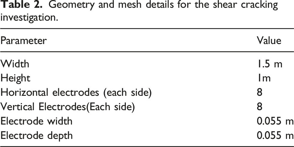
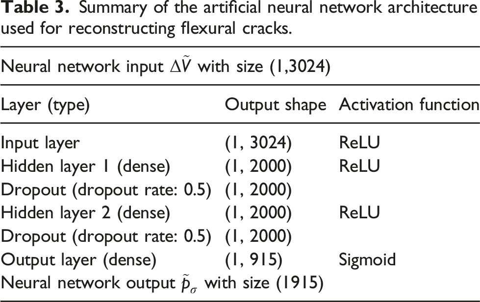
The discretizations for both investigations are shown in Figures 1 and 2. Spacing and locations of electrodes can be seen in the meshes with reference to Tables 1 and 2. In all cases, internal conductivity distributions were mapped on the discretizations in order to form a continuous distribution within the domain. For this, prior Gaussian background conductivity information was incorporated when generating the samples. In generating homogeneous backgrounds, conductivities in the range of 8–10 mScm⁻¹ were assumed in order to mimic realistic silver sensing skins (following Reference 69) in the flexural case as well as incorporating isotropic smoothness with a correlating length of 4 cm to incorporate spatial inhomogeneity. In the case of shear cracking, homogeneous background of 0.1 mScm⁻¹ was reasonably assumed in all instances to simulate potentially low-conductive large elements (Tables 3–5).

Figure 1.

Domain discretization for the flexural cracking investigation consisting of 2557 nodes and 4896 elements.

Figure 2.

Domain discretization for the shear cracking investigation consisting of 5047 nodes and 9680 elements.

Table 3.

Summary of the artificial neural network architecture used for reconstructing flexural cracks.

Neural network input $Δ \tilde{V}$ with size (1,3024)
Layer (type)	Output shape	Activation function
Input layer	(1, 3024)	ReLU
Hidden layer 1 (dense)	(1, 2000)	ReLU
Dropout (dropout rate: 0.5)	(1, 2000)
Hidden layer 2 (dense)	(1, 2000)	ReLU
Dropout (dropout rate: 0.5)	(1, 2000)
Output layer (dense)	(1, 915)	Sigmoid
Neural network output ${\tilde{p}}_{σ}$ with size (1915)

Table 4.

Summary of artificial neural network architecture used for reconstructing shear cracks.

Neural network input $Δ \tilde{V}$ with size (1,3024)
Layer (type)	Output shape	Activation function
Input layer	(1, 3024)	ELU
Hidden layer 1 (dense)	(1, 900)	ELU
Dropout (dropout rate: 0.5)	(1, 900)
Hidden layer 2 (dense)	(1, 900)	ELU
Dropout (dropout rate: 0.5)	(1, 900)
Output layer (dense)	(1, 1148)	Sigmoid
Neural network output ${\tilde{p}}_{σ}$ with size (1,1148)

Table 5.

Summary of convolutional neural network architecture used for reconstructing shear cracks.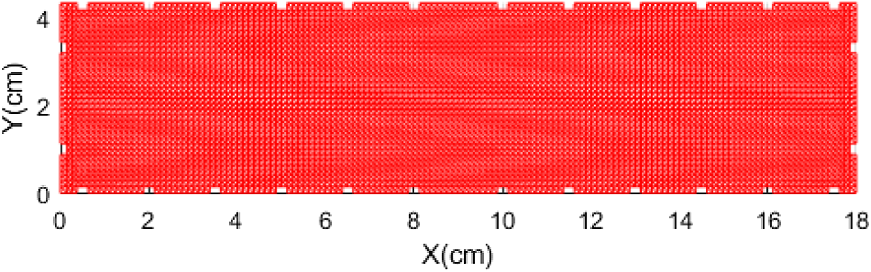

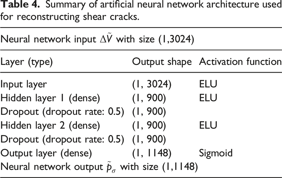
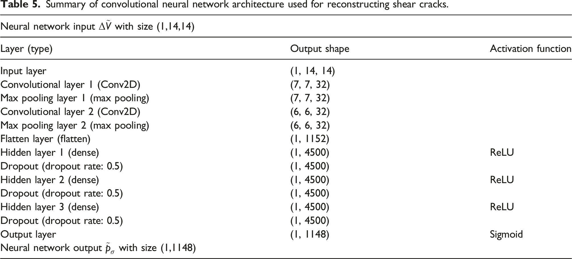
Neural network input $Δ \tilde{V}$ with size (1,14,14)
Layer (type)	Output shape	Activation function
Input layer	(1, 14, 14)
Convolutional layer 1 (Conv2D)	(7, 7, 32)
Max pooling layer 1 (max pooling)	(7, 7, 32)
Convolutional layer 2 (Conv2D)	(6, 6, 32)
Max pooling layer 2 (max pooling)	(6, 6, 32)
Flatten layer (flatten)	(1, 1152)
Hidden layer 1 (dense)	(1, 4500)	ReLU
Dropout (dropout rate: 0.5)	(1, 4500)
Hidden layer 2 (dense)	(1, 4500)	ReLU
Dropout (dropout rate: 0.5)	(1, 4500)
Hidden layer 3 (dense)	(1, 4500)	ReLU
Dropout (dropout rate: 0.5)	(1, 4500)
Output layer	(1, 1148)	Sigmoid
Neural network output ${\tilde{p}}_{σ}$ with size (1,1148)

In order to simulate measurement data with the ERT forward model, we adopt opposite current injection patterns while voltage measurements were taken via adjacent electrode pairs. Each flexural crack training sample consists of 3024 voltage measurements and a corresponding conductivity vector with 5047 (nodal) entries. Downsampled flexural crack training samples consist of the same number of measurements; however, the size of conductivity vector is reduced to 915 entries using bi-linear interpolation. Similarly, shear crack training samples consist of 196 voltage measurements (which are reshaped to the 14 × 14 input size for use in CNNs). Additionally, each shear crack training sample also contains a conductivity vector having 1148 entries. Lastly, 2% Gaussian noise was added to all voltage and conductivity training data sets to improve regularization, prevent over fitting and improve network generalizability.^70–72

Crack pattern generation

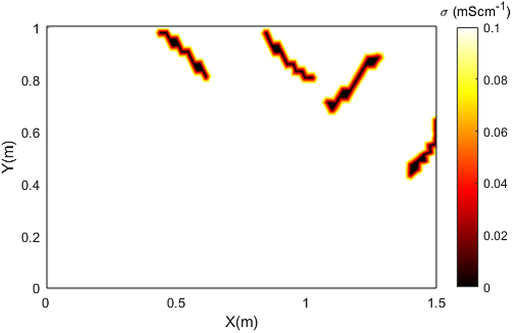
In order to train the NNs, artificial cracks need to be generated and incorporated into the training samples. For the flexural cracking training set generation, cracks were initialized at the bottom of the domain using prior knowledge of the loading and boundary conditions (i.e. three-point bending). For this, generators consisting of one or two cracks were initialized at different starting locations with various progressing directions. Cracks were simulated by random incremental steps of which the total number is randomized, leading to cracks that could reach arbitrary length within the boundary, such that a sufficient number of training samples were available. Meanwhile, shear cracks were initialized within the domain, while crack progression directions were controlled within a range of 0–45° resulting from the experimental shear testing boundary condition information. Representative internal conductivity distributions for both cracking mechanisms are shown in Figures 3 and 4.

Figure 3.

Sample conductivity distribution used in flexural cracking training data.

Figure 4.

Sample conductivity distribution used in shear cracking training data.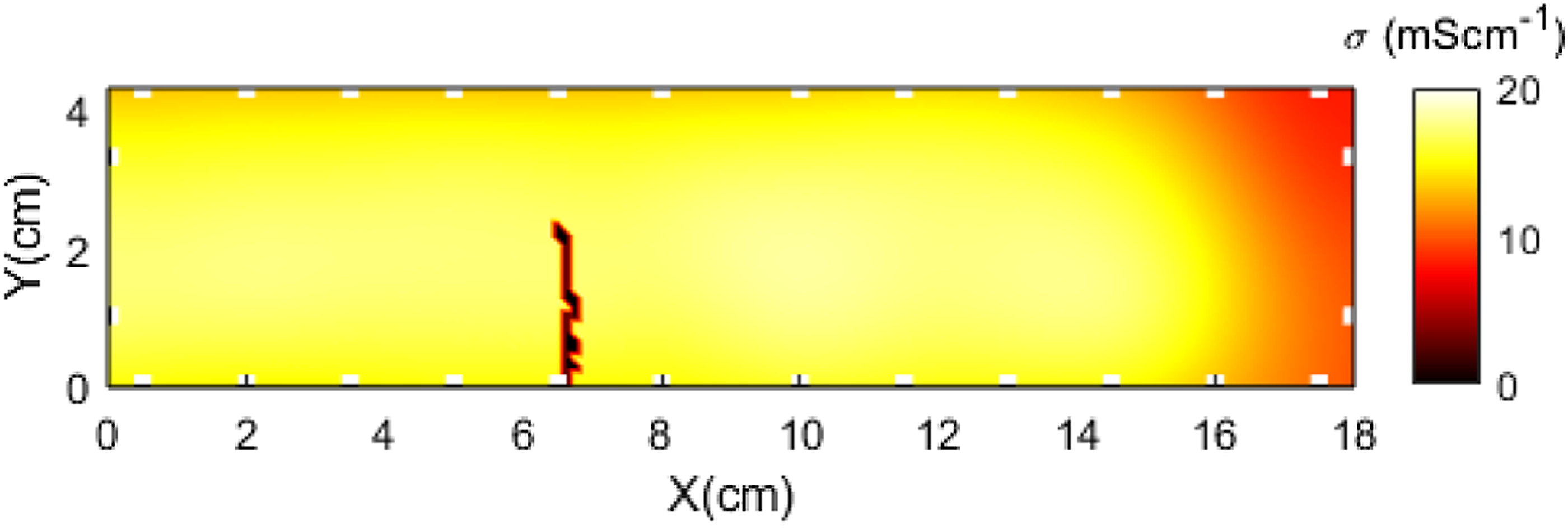

Data processing and training

As indicated previously, the aim of the network training process is to learn the nonlinear mapping between ERT difference measurements and binary crack distributions. To do this, Keras⁷³ is implemented in a Python environment for both generating NN architectures and training. In training an individual NN, 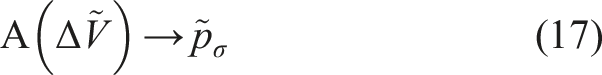$A$ , we utilize t ∈ N training data comprising $Δ \tilde{V}$ and ${\tilde{p}}_{σ}$ where the tilde denotes training data. This process can be holistically written as

A (Δ \tilde{V}) \to {\tilde{p}}_{σ}

(17)

Based on this information, we may now explicitly write the desired training loss function as follows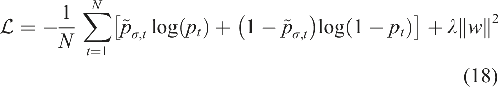

ℒ = - \frac{1}{N} \sum_{t = 1}^{N} [{\tilde{p}}_{σ, t} \log (p_{t}) + (1 - {\tilde{p}}_{σ, t}) \log (1 - p_{t})] + λ {‖ w ‖}^{2}

(18)

The preceding loss function minimization is augmented with a dropout rate of 50%, effectively supplementing L₂ weight regularization and noise addition to data, to further improve network generalizability and prevent over fitting.⁷⁴

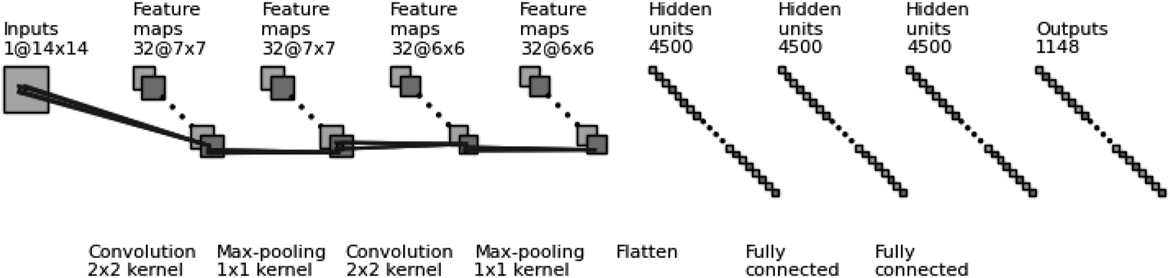
Regarding the generated training data, the overall dimensionality of both inputs $(Δ \tilde{V})$ and outputs $({\tilde{p}}_{σ})$ is immense due to (a) the fine discretizations and (b) the large number of measurements used. Hence, a spatially interpolated downsampling step is additionally considered in order to map the high-fidelity distributions of ${\tilde{p}}_{σ}$ onto a smaller nodal space, thus aiming to reduce the overall dimensionality of this mapping task for the NN. Such a reduction is expected to result in a reduced error space during gradient decent process.

Owing to the fact that the dimensionality of $Δ \tilde{V}$ is significantly smaller than ${\tilde{p}}_{σ}$ (a common feature in ERT), the training process effectively stretches and amplifies information in $Δ \tilde{V}$ via NN throughput of $Δ \tilde{V} \to {\tilde{p}}_{σ}$ . Therefore, given the dimensionality mismatches, the design of NN architectures is conducted via trial and error. To this end, an ANN is applied for both flexural and shear cracking applications while the use of a CNN is explored for reconstructing shear cracking alone. Regarding the latter, the central reason for not utilizing a CNN for flexural cracking predictions is owed to realizations made during preliminary trial and error processes – namely, that ANNs of basic architectural complexity were sufficient for flexural cracking predictions thereby negating the need for computationally demanding CNN training. Schematic ANN and CNN architectures are provided in Figures 5 and 6, respectively.

Figure 5.

Schematic trained artificial neural network architecture.

Figure 6.

Schematic trained convolutional neural network architecture.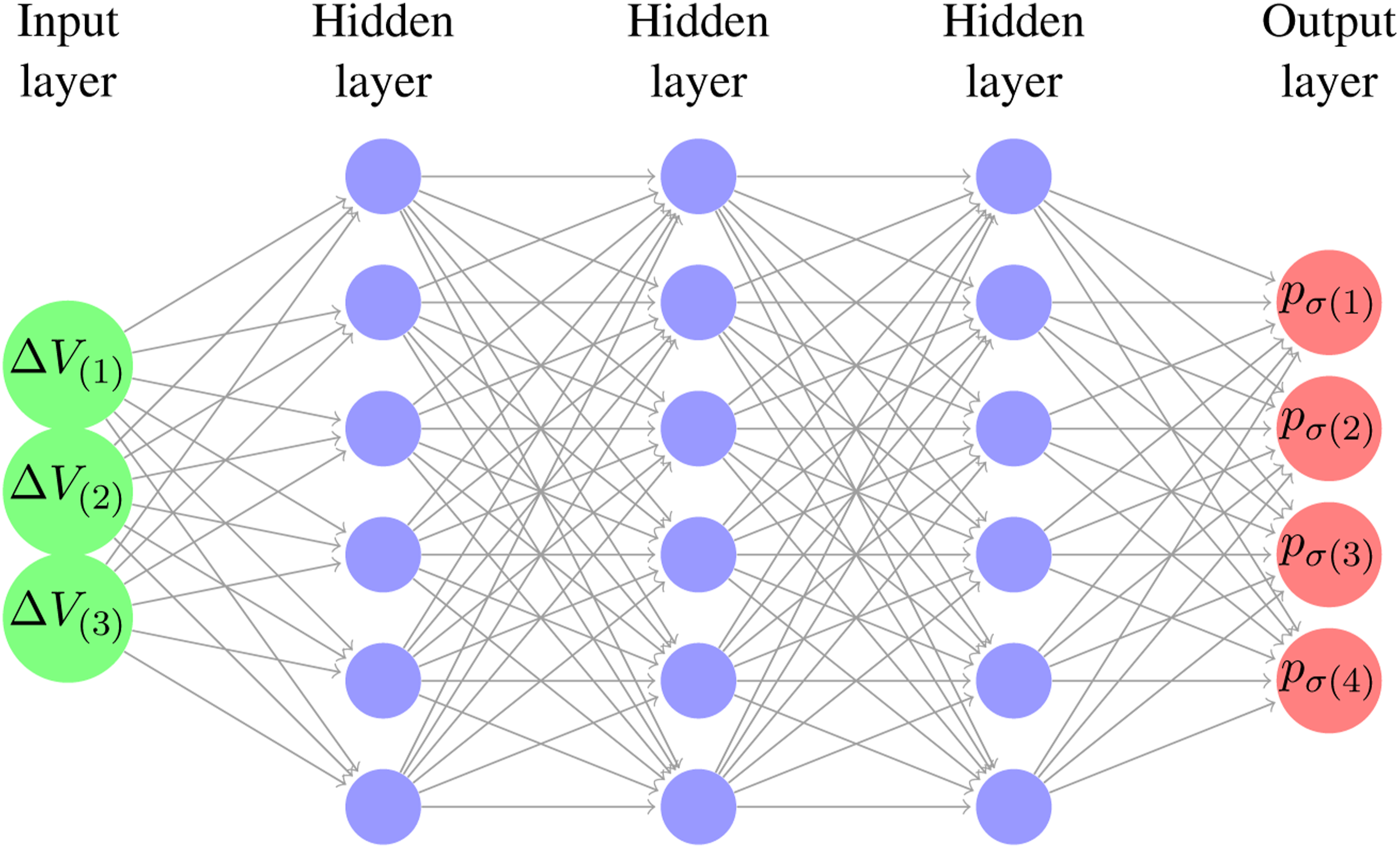

The finalized ANN architecture used for flexural crack predictions is comprised of one input layer, two hidden layers each consisting of 2000 neurons equipped with ReLU activation functions, and an output layer consistent with the number of entries in an individual sample in ${\tilde{p}}_{σ}$ . Additionally, the ANN architecture for shear cracking predictions includes three hidden layers of each consisting of 900 neurons with ELU activation functions followed by output layer with the same number of entries in an individual sample in ${\tilde{p}}_{σ}$ . Procedurally, the ANN training processes are set to stop when the loss function for validation data consisting of 5000 independent samples exceeded a patience of 100 epochs.

Unlike in the straightforward implementation of ANNs where we map a vector to a vector, we utilize image-based CNNs. As such, we require a rectangular input; consequently, we choose to reshape the input data $Δ \tilde{V}$ to a 14 × 14 matrix form. This information is then fed into one convolutional layer with 32 filters having a kernel size of 2 × 2 followed by a 1 × 1 max pooling layer. Secondly, the same sets of convolutional and max pooling layers were added. Then, a flatten layer was added before a fully connected ANN structure consisting of three hidden layers with 4500 neurons each. ReLU activation functions were used in hidden layers while sigmoid functions were applied in the output layer. In training, 5000 samples were utilized and found to be sufficient to adequately train the network. However, in previous trial and error procedures, it was found that significant computational resources were needed in order to optimize the CNN parameters. This was owed to the lack of distinguishability in input voltage data corresponding to conductivity changes central region of the domain (a common sensitivity issue in ERT).

Based on the former preliminary realizations, we propose and investigate an alternative approach to CNN predictions where the conductivity vector is segmented to five pieces. As a result, five different NNs are trained and developed with reduced dimensionality aiming at improving prediction accuracy for individual segments and overall domain predictions after the final assembly of segments. Another advantage of this methodology relates to regions where information is poor – especially the central region – where (a) more training samples can be added or (b) other parameters could be adjusted to improve the training performance avoiding the need to retrain a large (entire domain) CNN.

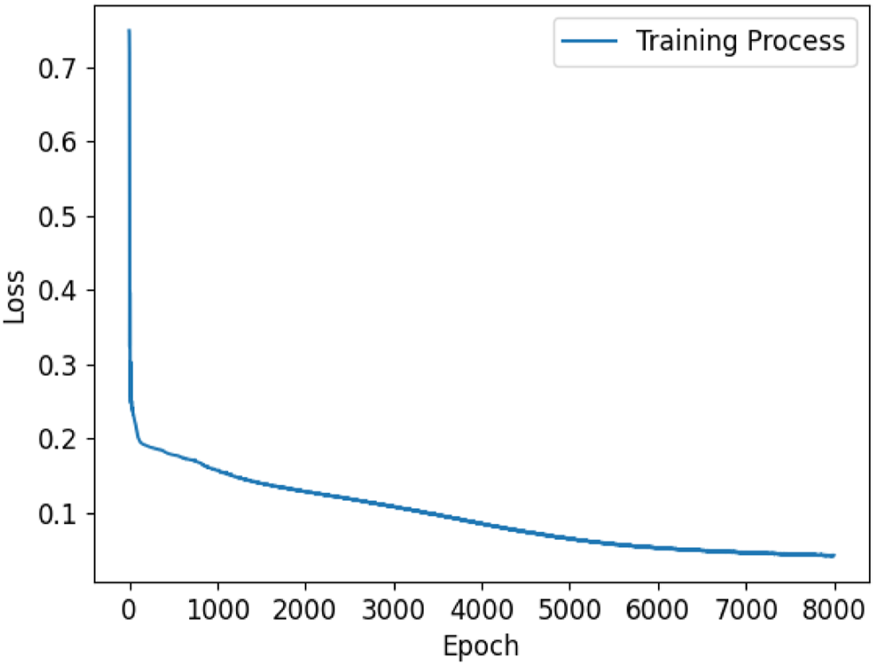
Lastly, to provide more detailed information on network training, Figures 7 and 8 show the training processes for two typical NNs. In these figures, we observe a near immediate reduction in the loss indicating rapid learning. Following this initial phase, a gradual decrease in the loss function is observed, characterized by fine-tuning of the network weights and biases. It is worth noting here that, since different network architectures and training samples are used in this work, the number of epochs varies needed to reach respective stopping criteria varies significantly.

Figure 7.

Loss function minimization for an artificial neural network used in this work.

Figure 8.

Loss function minimization for a convolutional neural network used in this work (non-segmented data).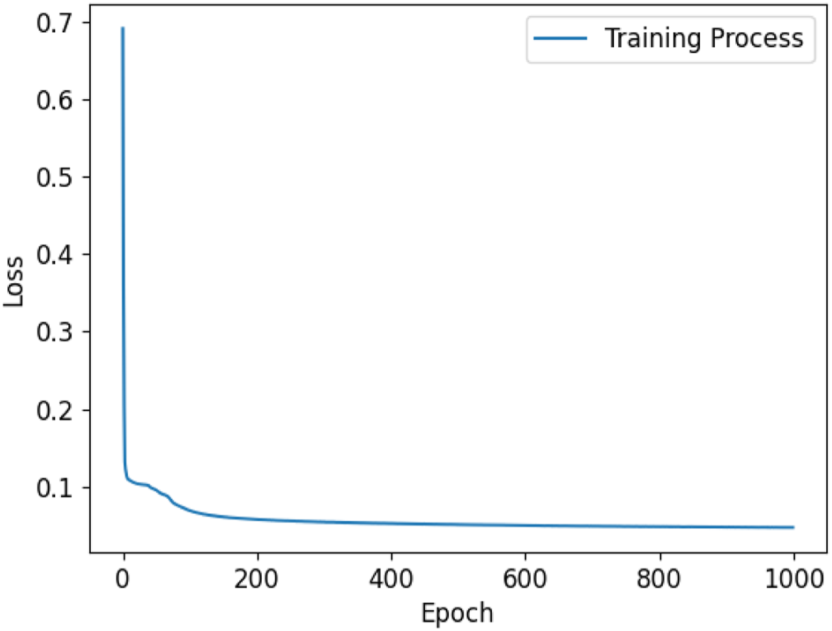

Results and discussion

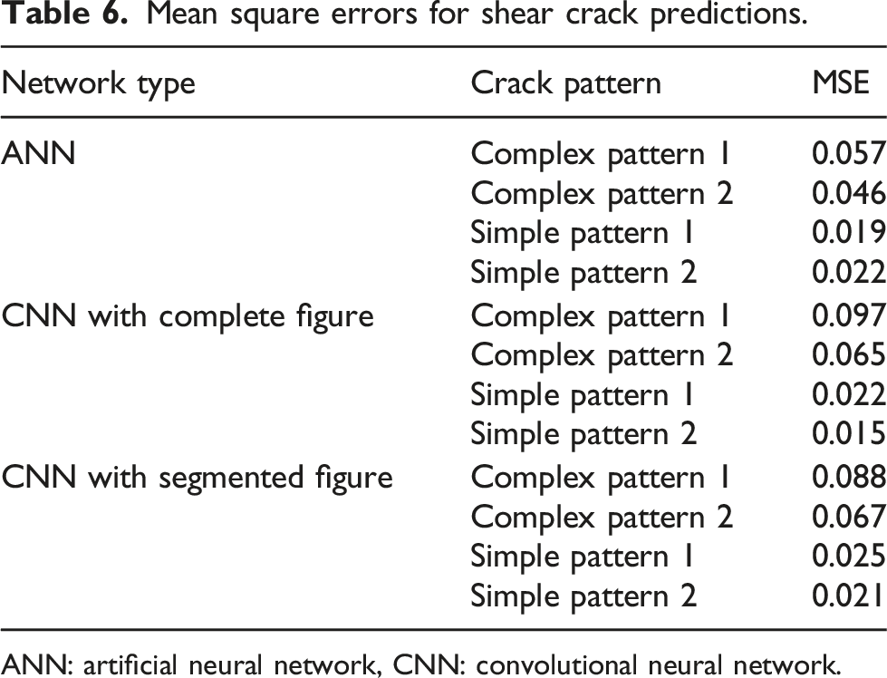
In this section, we report and discuss cracking predictions from experimental flexural and simulated shear testing campaigns. Tabulated images showing these cracking predictions are reported in Figures 9 and 10. In the spatial mappings reported, colour bars represent the probability of cracks existing at a nodal location. For the purpose of quantitative comparison, the mean square error (MSE) metric, measured between the predictive results and simulated results, for shear cracks are summarized in Table 6. In the forthcoming subsection, we will detail results for flexural testing, followed by a subsection detailing shear testing predictions, and lastly, discussion will be provided.

Figure 9.

NN predictions of experimental flexural cracking patterns.

Figure 10.

NN predictions of simulated shear cracking patterns.

Table 6.

Mean square errors for shear crack predictions.

Network type	Crack pattern	MSE
ANN	Complex pattern 1	0.057
	Complex pattern 2	0.046
	Simple pattern 1	0.019
	Simple pattern 2	0.022
CNN with complete figure	Complex pattern 1	0.097
	Complex pattern 2	0.065
	Simple pattern 1	0.022
	Simple pattern 2	0.015
CNN with segmented figure	Complex pattern 1	0.088
	Complex pattern 2	0.067
	Simple pattern 1	0.025
	Simple pattern 2	0.021

ANN: artificial neural network, CNN: convolutional neural network.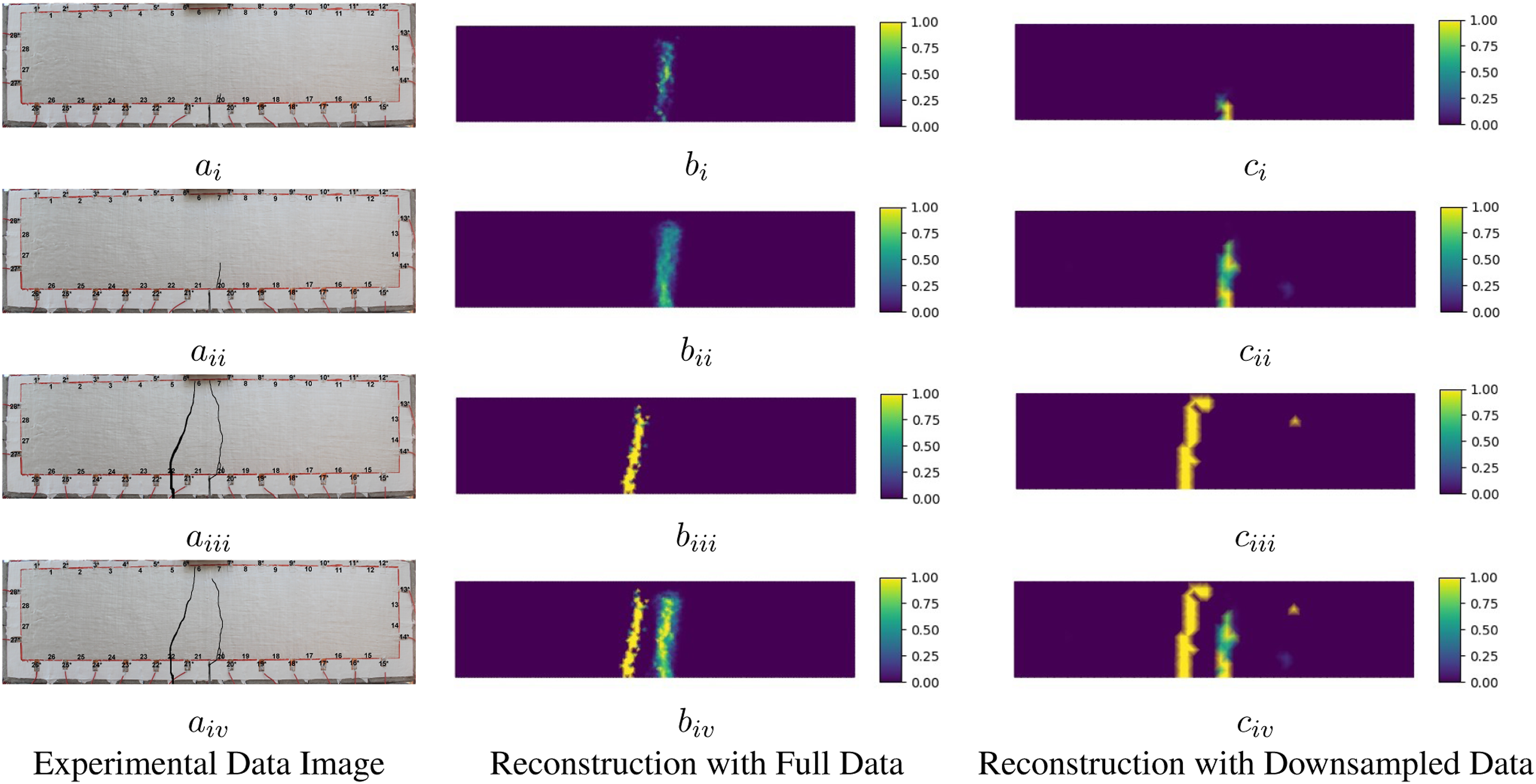

Flexural crack reconstruction

Flexural cracking predictions are shown in Figure 9 alongside experimental photographs with highlighted crack. Column a shows the experimental photographs, column b shows the crack predictions based on full conductivity sampling, and column c reports predictions using based on downsampled conductivity. Generally speaking, NN predictions correctly localize the initial crack topology (top row) in comparison to the experimental photographs as observed in a_i, b_i and c_i. In addition, crack growth can be observed in b_ii and c_ii for both data types while the downsampled data prediction visually outperforms the full data prediction in terms of the actual length of the growing crack. In b_iii and c_iii, only a single crack can be observed, which matches the left crack shown in a_iii. Further, in b_iv and c_iv, both the full and downsampled predictions accurately capture both cracks.

As a whole, we observe improved predictions when utilizing downsampled data. It is worth nothing, however, that this qualitative observation comes at a loss of spatial resolution in predictions p_σ. It can also be observed that in predictions b_iii and v_iii, the reconstructions do not capture the right crack, irrespective of sampling fidelity, this drawback can be potentially explained by the presence of the left crack, which effectively shields electric fields and leads to a reduction in measurement information needed in resolving the right crack.¹³ In addition, the inability to accurately predict the right crack in the third row could also be due to the relatively large width to depth ratio of this domain, where electric fields flowing horizontally are, in as rough sense, more constrained than in geometries having aspect ratios approaching 1:1. Moreover, the presence of small artifacts can be observed in c_iii and c_iv which result from NN predictive errors (a function of, for example, measurement noise and geometrical discretization error); however, these errors are small relative to topological crack prediction errors and do not significantly corrupt the overall assessment of crack predictions.

Shear crack reconstruction

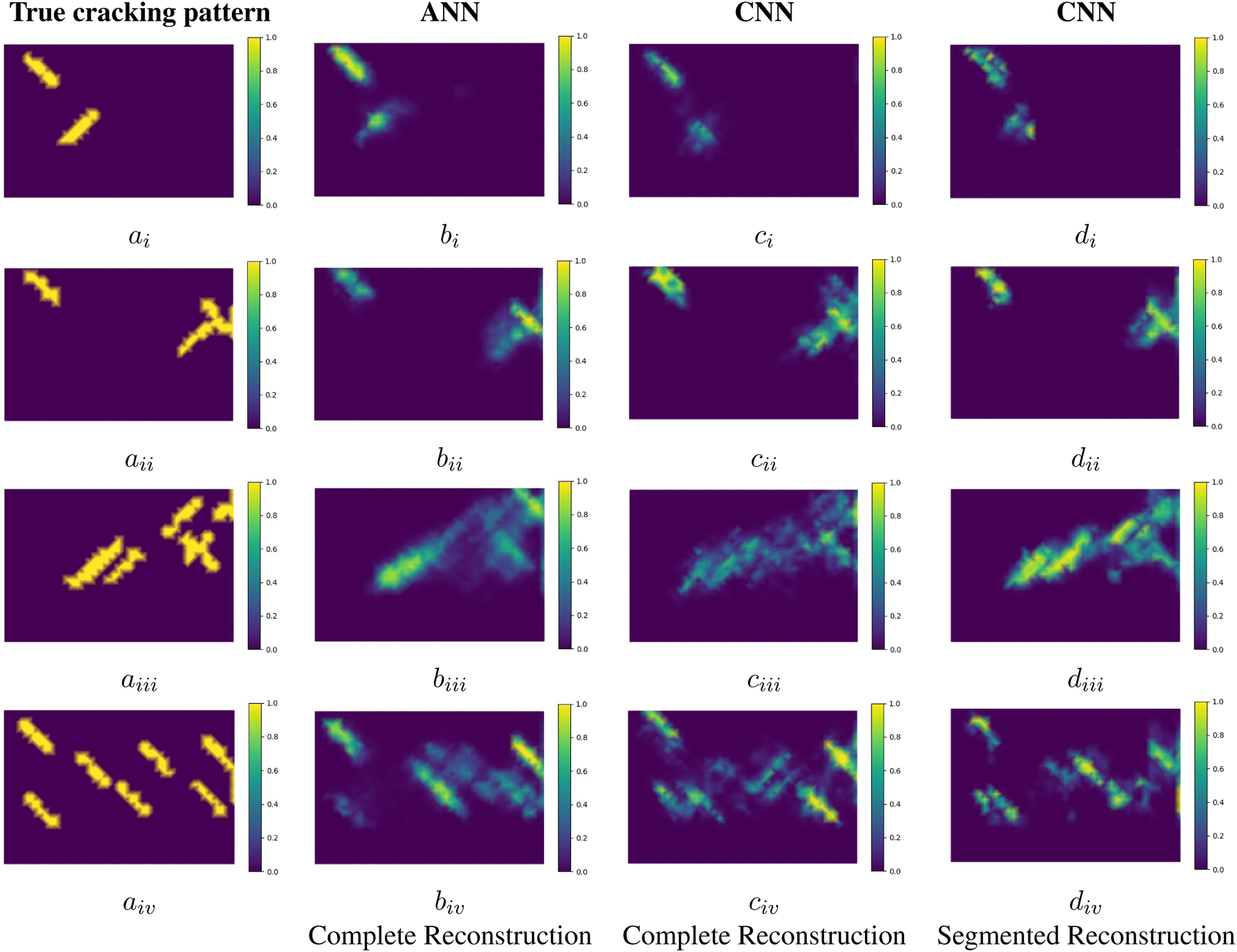
Artificial neural network and CNN shear cracking predictions based on downsampled data are reported in Figure 10. Column a shows the true cracking binary representation. Column b reports ANN predictions for the entire domain. Column c reports CNN predictions results for the entire domain. Lastly, column d reports segmented CNN predictions. In addition, consolidating five segmented networks. In total, four differing cracking patterns of increasing complexity are considered (least complexity in the top row and most complexity in the bottom row).

Generally speaking, for simple crack patterns (i.e. the first and second rows), both the ANNs and CNNs provide valid predictions in terms of crack lengths and locations. However, when observed in closer detail, the ANN visually outperforms the CNN predictions slightly as in b_i and b_ii where the length of cracks are more accurately predicted. For more complex crack patterns (i.e. the third and fourth rows), all NN cracking predictions are satisfactory near the domain boundaries. On the other hand, near the centre of the domains (the area of least sensitivity), CNNs appear to localize and separate complex cracks better than ANNs as observed from c_iii, d_iii c_iv and d_iv. Furthermore, segmented CNN predictions consistently show improved qualitative results in comparison to the conventional CNN network.

In totality, both the ANNs and CNNs predict less accurately towards the central region of the domain relative to the boundary. This is likely caused by the diffusive nature of electricity and is also a common feature of ERT.³⁹ However, despite the generally better qualitative results predicted by CNNs, we require a quantitative metric to more closely assess predictions. For this, we utilize the MSE metric, effectively comparing true and predicted images; these metrics are reported in Table 6.

In contrast to visual observations, assessment of MSEs reported in Table 6 indicates that ANNs generally perform quantitatively slightly better than CNNs – with the notable exception of one cracking pattern. This could potentially be due to fact that the CNNs’ architecture and data processing add additional nonlinearity in the training and prediction process. While this initially seems counterintuitive, as CNNs are commonly regarded as more powerful predictive tools than ANNs, additional discussion is required to attain a more full picture of the realizations made in this subsection. Such discussion will be provided henceforth.

Discussion

The feasibility of NNs for probabilistically predicting cracking patterns was qualitatively and quantitatively affirmed in the preceding subsections using experimental and simulated data. Generally speaking, the networks were able to localize binary crack representations with regional certainty exceeding 50% – with the notable exception of cases where measurement quality was impeded by crack shielding. As alluded to, the use of NNs for predicting cracks using boundary voltage measurements is analogous to ERT, with the caveat that the learned methodology proposed herein predicts binary cracking representations rather than reconstructing continuous conductivity distributions. Interestingly, the proposed NN crack prediction framework also exhibits similar susceptibilities present in ERT; the primary weaknesses include (a) insensitivity to the central region of the prediction domain and (b) low spatial resolution. Conversely, and again similar to ERT, the NN prediction framework also has analogous advantages including (i) high sensitivity near the boundaries and high temporal resolution. In contrast to ERT, however, the NN prediction framework enables substantial computational speedups and simpler representation of cracking topology relative to conventional ERT.

Despite the noted advantages, two observations made in the results subsections remain yet to be explained. Realizations from these observations have key implications on the potential use of predictive networks for probabilistic crack assessment in future work. Firstly, the use of spatial downsampling proved highly effective and generally improved prediction quality. Secondly, the use of CNNs, commonly considered a more powerful classification network, only outperformed ANNs in one case considered.

In response to the first observation, we need to first investigate the general structure of input and output data sets used herein. We note that, when binary crack representation data (output) are not downsampled, the output dimensionality is an order of magnitude larger than input measurement data. As such, information stemming from measurements is significantly diffused and stretched before reaching the outputs. This is similar to the process of decoding, that is, mapping low dimensional information to high dimensional information, as commonly adopted in autoencoder applications.^75,76 A primary challenge presented in the decoding process lies in the preservation of information transferred from input to output. Potential for corruption in decoding, however, can be reduced by optimizing the NN architecture and decreasing discrepancy between input/output data size. Regarding the latter, downsampling of the outputs (as used herein) is an effective method for matching data sizing discrepancies and therefore underscores the effectiveness of downsampling in crack prediction quality observed.

Responding to the second observation, regarding the reduced effectiveness of CNN cracking predictions in comparison to those of ANNs, we would like to remark that this was an unexpected result. Nowadays, applications of CNNs range from image processing to inverse problems. Recent scholarly work has even investigated the ‘unreasonable effectiveness of CNNs’.⁷⁷ Yet, like many machine learning tools, the use of specific architectures and data processing techniques should be considered with respect to the application and underlying data structure(s).

In this work, the input data (potential differences) may have a positive or negative sign and the magnitude can vary significantly, depending on the cracking pattern, domain geometry, electrode configuration, and measurement/stimulation protocol. In turn, reshaping such data into a rectangular ‘voltage image’ unquestionably represents a much more complex data structure than if it were, for example, a black and white image consisting of positive integer values ranging from 0 to 255. Therefore, the use of convolutional operations in comparison to feed-forward (ANN) operations may not be ideal in many cases. Such a realization may contribute to the fact that CNNs performed less favourably than ANNs in predicting all but one cracking representation.

The former deduction is not a general conclusion of this work, however, as CNNs (and fully connected networks) offer opportunities for deeper data representation. For example, derivative operations have equivalencies to convolution operations^78,79 meaning that higher order data representations are possible using CNNs. Therefore, the use of deeper non-fully connected networks highly tailored to data and prediction may, in eventuality, lead to substantially improved predictions of cracking representations than those reported herein, and this is the source of ongoing research.

Conclusions

In this article, fast neural network–driven direct inversion frameworks were proposed to predict binary cracking distributions in concrete elements. The aim of the proposed framework was to map boundary electrical measurements to probabilistic binary crack distributions. The purpose for choosing a binary cracking representation was to simplify the interpretability of damage predictions. To test the feasibility of the approach, experimental flexural cracking representations were successfully predicted with using ANNs. To facilitate quantitative evaluation of networks’ efficacy, simulated shear cracking representations were predicted using ANNs and CNNs. Simulation results generally indicated that ANNs slightly outperformed CNNs quantitatively, while both architectures showed the potential to accurately reconstruct simple and complex crack patterns. In summary, the feasibility of the proposed learned frameworks was affirmed and discussion was provided to offer guidance on the potential for improving network predictions.

Footnotes

Acknowledgements

DS thanks Professor Moe Pour-Ghaz (North Carolina State University), Professor Aku Seppänen (University of Eastern Finland) and Dr Milad Hallaji (Fernandez & Associates) for providing experimental data.

Declaration of conflicting interests

The author(s) declared no potential conflicts of interest with respect to the research, authorship, and/or publication of this article.

Funding

The author(s) disclosed receipt of the following financial support for the research, authorship, and/or publication of this article: DS was supported by Engineering and Physical Sciences Research Council Project EP/V007025/1. DL was supported by the National Natural Science Foundation of China under Grant 61871356.

ORCID iDs

Dong Liu

Danny Smyl

References

Balageas

Fritzen

Güemes

. Structural health monitoring, volume 90. Chichester, West Sussex: John Wiley & Sons, 2010.

Farrar

Worden

. Structural Health Monitoring: A Machine Learning Perspective. Chichester, West Sussex: John Wiley & Sons, 2012.

Gholizadeh

. A review of non-destructive testing methods of composite materials. Procedia Structural Integrity 2016; 1: 50–57.

Mutlib

Baharom

El-Shafie

, et al, Ultrasonic health monitoring in structural engineering: buildings and bridges. Structural Control and Health Monitoring 2016; 23(3): 409–422.

Montinaro

Cerniglia

Pitarresi

. Evaluation of interlaminar delaminations in titanium-graphite fibre metal laminates by infrared ndt techniques. NDT & E International 2018; 98: 134–146.

Kong

. Vision-based fatigue crack detection of steel structures using video feature tracking. Computer-Aided Civil and Infrastructure Engineering 2018; 33(9): 783–799.

. Experimental and analytical studies on h-shaped reinforced concrete squat walls. ACI Structural Journal 2018; 115(2): 425–438.

Smyl

. Electrical tomography for characterizing transport properties in cement-based materials: a review. Construction and Building Materials 2020; 244: 118299.

Karhunen

Seppänen

Lehikoinen

, et al. Electrical resistance tomography imaging of concrete. Cement and Concrete Research 2010; 40(1): 137–145. DOI: 10.1016/j.cemconres.2009.08.023.

10.

Pour-Ghaz

Niemuth

Weiss

. Use of electrical impedance spectroscopy and conductive surface films to detect cracking and damage in cement based materials. Special Publication 2013; 292: 1–16.

11.

McCarter

Garvin

. Dependence of electrical impedance of cement-based materials on their moisture condition. Journal of Physics D: Applied Physics 1989; 22(11): 1773–1776.

12.

Zhou

Bhat

Ouyang

, et al. Localization of cracks in cementitious materials under uniaxial tension with electrical resistance tomography. Construction and Building Materials 2017; 138: 45–55.

13.

Smyl

Pour-Ghaz

Seppänen

. Detection and reconstruction of complex structural cracking patterns with electrical imaging. NDT & E International 2018; 99: 123–133.

14.

Shi

Guan

. Detection of crack development in steel fibre engineered cementitious composite using electrical resistivity tomography. Smart Materials and Structures 2019; 28(12): 125011.

15.

Liu

Smyl

. Nonstationary shape estimation in electrical impedance tomography using a parametric level set-based extended kalman filter approach. IEEE Transactions on Instrumentation and Measurement 2020; 69(5): 1894–1907.

16.

Smyl

Bossuyt

Ahmad

, et al. An overview of 38 least squares-based frameworks for structural damage tomography. Structural Health Monitoring 2020; 19(1): 215–239.

17.

Rashetnia

Alla

Gonzalez-Berrios

, et al. Electrical resistance tomography–based sensing skin with internal electrodes for crack detection in large structures. Materials Evaluation 2018; 76(10): 1405–1413.

18.

Kröse

Krose

van der Smagt

, et al. An Introduction to Neural Networks, 1993 Amsterdam, the Netherlands: The University of Amsterdam.

19.

Papert

. Some mathematical models of learning. In: Proceedings of the fourth London symposium on information theory, London, 1960.

20.

Baum

. On the capabilities of multilayer perceptrons. Journal of complexity 1988; 4(3): 193–215.

21.

Bishop

. Neural Networks for Pattern Recognition. Oxford: Oxford University Press, 1995.

22.

LeCun

Bengio

Hinton

. Deep learning. nature 2015; 521(7553): 436–444.

23.

LeCun

Boser

Denker

, et al. Backpropagation applied to handwritten zip code recognition. Neural Computation 1989; 1(4): 541–551.

24.

Luo

Roads

Love

. The costs and benefits of goal-directed attention in deep convolutional neural networks. Computational Brain & Behavior 2021; 4(2): 213–230.

25.

LeCun

Bengio

, et al. Convolutional networks for images, speech, and time series. The handbook of Brain Theory and Neural Networks 1995; 3361(10): 1995.

26.

O’Shea

Nash

. An Introduction to Convolutional Neural Networks. arXiv preprint arXiv:151108458 2015.

27.

Goodfellow

Bengio

Courville

, et al. Deep learning, vol 1. MIT press Cambridge, 2016.

28.

Albawi

Mohammed

Al-Zawi

. Understanding of a convolutional neural network. In: International conference on engineering and technology (ICET), Antalya, Turkey, 08 March 2018, pp. 1–6. IEEE, 2017.

29.

Saxe

Berlin

. Deep neural network based malware detection using two dimensional binary program features. In: 10th international conference on malicious and unwanted software (MALWARE), Fajardo, PR, USA, 20-22 October 2015, pp. 11–20. IEEE, 2015.

30.

Hopfield

. Neural networks and physical systems with emergent collective computational abilities. Proceedings of the Nationall Academy of Sciences 1982; 79(8): 2554–2558.

31.

Ackley

Hinton

Sejnowski

. A learning algorithm for boltzmann machines*. Cognitive Science 1985; 9(1): 147–169.

32.

Lee

, et al. Gradient descent finds global minima of deep neural networks. In: International conference on machine learning. Long Beach, CA, 09-15 June 2019, pp. 1675–1685. PMLR.

33.

Bao

Guo

. A machine learning-based approach for adaptive sparse time-frequency analysis used in structural health monitoring. Structural Health Monitoring 2020; 19(6): 1963–1975.

34.

Mousavi

Varahram

Ettefagh

, et al. Deep neural networks–based damage detection using vibration signals of finite element model and real intact state: An evaluation via a lab-scale offshore jacket structure. Structural Health Monitoring 2020; 20(1): 379-405. DOI: 10.1177/1475921720932614.

35.

Glisic

Kim

, et al. Convolutional neural network-based data recovery method for structural health monitoring. Structural Health Monitoring 2020; 19(6): 1821–1838.

36.

Mohtasham Khani

Vahidnia

Ghasemzadeh

, et al. Deep-learning-based crack detection with applications for the structural health monitoring of gas turbines. Structural Health Monitoring 2020; 19(5): 1440–1452.

37.

Henderson

Webster

. An impedance camera for spatially specific measurements of the thorax. IEEE Transactions on Biomedical Engineering 1978; 25(3): 250–254.

38.

Yang

York

. New ac-based capacitance tomography system. IEE Proceedings - Science, Measurement and Technology 1999; 146(1): 47–53.

39.

Hallaji

Seppänen

Pour-Ghaz

. Electrical impedance tomography-based sensing skin for quantitative imaging of damage in concrete. Smart Materials and Structures 2014; 23(8): 085001.

40.

Smyl

Liu

. Damage tomography as a state estimation problem: crack detection using conductive area sensors. IEEE Sensors Letters 2019; 3(10): 1–4.

41.

Loh

Kim

Lynch

, et al. Multifunctional layer-by-layer carbon nanotube-polyelectrolyte thin films for strain and corrosion sensing. Smart Materials and Structures 2007; 16(2): 429–438.

42.

Loh

Hou

T-C

Lynch

, et al. Carbon nanotube sensing skins for spatial strain and impact damage identification. Journal of nondestructive Evaluation 2009; 28(1): 9–25.

43.

Loyola

Briggs

Arronche

, et al. Detection of spatially distributed damage in fiber-reinforced polymer composites. Structural Health Monitoring 2013; 12(3): 225–239.

44.

Lestari

Pinto

La Saponara

, et al. Sensing uniaxial tensile damage in fiber-reinforced polymer composites using electrical resistance tomography. Smart Materials and Structures 2016; 25(8): 085016.

45.

Tallman

Gungor

Koo

, et al. On the inverse determination of displacements, strains, and stresses in a carbon nanofiber/polyurethane nanocomposite from conductivity data obtained via electrical impedance tomography. Journal of Intelligent Material Systems and Structures 2017; 28(18): 2617–2629.

46.

Tallman

Gungor

Wang

, et al. Damage detection and conductivity evolution in carbon nanofiber epoxy via electrical impedance tomography. Smart Materials and Structures 2014; 23(4): 045034.

47.

Tallman

Smyl

. Structural health and condition monitoring via electrical impedance tomography in self-sensing materials: a review. Smart Materials and Structures 2020; 29(12): 123001.

48.

Hassan

Tallman

. Failure prediction in self-sensing nanocomposites via genetic algorithm-enabled piezoresistive inversion. Structural Health Monitoring 2020; 19(3): 765–780.

49.

Hallaji

Seppänen

Pour-Ghaz

. Electrical resistance tomography to monitor unsaturated moisture flow in cementitious materials. Cement and Concrete Research 2015; 69: 10–18.

50.

Liu

Smyl

, et al. Shape-driven difference electrical impedance tomography. IEEE Transactions on Medical Imaging 2020; 39(12): 3801–3812.

51.

Fan

Ying

. Solving electrical impedance tomography with deep learning. Journal of Computational Physics 2020; 404: 109119.

52.

Tan

Dong

, et al. Image reconstruction based on convolutional neural network for electrical resistance tomography. IEEE Sensors Journal 2018; 19(1): 196–204.

53.

Hamilton

Hauptmann

. Deep d-bar: real-time electrical impedance tomography imaging with deep neural networks. IEEE Transactins on Medical Imaging 2018; 37(10): 2367–2377.

54.

Smyl

Liu

. Optimizing electrode positions in 2-d electrical impedance tomography using deep learning. IEEE Transactions on Instrumentation and Measurement 2020; 69(9): 6030–6044.

55.

Kuo-Sheng Cheng

Isaacson

Newell

, et al. Electrode models for electric current computed tomography. IEEE Transactions on Biomedical Engineering 1989; 36(9): 918–924.

56.

Vauhkonen

Vadasz

Karjalainen

, et al. Tikhonov regularization and prior information in electrical impedance tomography. IEEE Transactions on Medical Imaging 1998; 17(2): 285–293.

57.

Vauhkonen

. Electrical Impedance Tomography and Prior Information 1997. Kuopio, Finland: Kuopio University Publications. C, Natural and environmental sciences.

58.

Liu

Smyl

. A parametric level set-based approach to difference imaging in electrical impedance tomography. IEEE Transactions on Medical Imaging 2019; 38(1): 145–155.

59.

Kotsiantis

Zaharakis

Pintelas

. Supervised machine learning: a review of classification techniques. Emerging Artificial intelligence Applications in Computer Engineering 2007; 160(1): 3–24.

60.

Osisanwo

Akinsola

Awodele

, et al. Supervised machine learning algorithms: classification and comparison. International Journal of Computer Trends and Technology (IJCTT) 2017; 48(3): 128–138.

61.

Cercone

. Discretization of continuous attributes for learning classification rules. In: Pacific-Asia Conference on Knowledge Discovery and Data Mining. Berlin, Heidelberg: Springer, pp. 509–514.

62.

Saad

. Online algorithms and stochastic approximations. Online Learning 1998; 5: 6–3.

63.

Cheng

Bell

Liu

. Learning bayesian networks from data: an efficient approach based on information theory. On World Wide Web at http://www.cs.ualberta.ca/˜.jcheng/bnpc.htm.1998.

64.

Liu

. Efficient feature selection via analysis of relevance and redundancy. The Journal of Machine Learning Research 2004; 5: 1205–1224.

65.

Smyl

Tallman

Black

, et al. Learning and correcting non-gaussian model errors. Journal of Computational Physics 2021; 432: 110152.

66.

Denton

Hung

Osyk

. A neural network approach to the classification problem. Expert Systems with Applications 1990; 1(4): 417–424.

67.

Jeatrakul

Wong

. Comparing the performance of different neural networks for binary classification problems. In: Eighth international symposium on natural language processing, Bangkok, Thailand, 20-22 October 2009, pp. 111–115. IEEE, 2009.

68.

Pasupa

Sunhem

. A comparison between shallow and deep architecture classifiers on small dataset. In: 8th International conference on information technology and electrical engineering (ICITEE), Yogyakarta, Indonesia, 5-6 October 2016, pp. 1–6. IEEE, 2016.

69.

Seppänen

Hallaji

Pour-Ghaz

. A functionally layered sensing skin for the detection of corrosive elements and cracking. Structural Health Monitoring 2017; 16(2): 215–224.

70.

Bishop

. Training with noise is equivalent to tikhonov regularization. Neural Computation 1995; 7(1): 108–116.

71.

Poole

Sohl-Dickstein

Ganguli

. Analyzing Noise in Autoencoders and Deep Networks. arXiv preprint arXiv:14061831 2014.

72.

Neelakantan

Vilnis

, et al. Adding Gradient Noise Improves Learning for Very Deep Networks. arXiv preprint arXiv:151106807 2015.

73.

Chollet

. keras. https://github.com/fchollet/keras 2015.

74.

Srivastava

Hinton

Krizhevsky

, et al. Dropout: a simple way to prevent neural networks from overfitting. The Journal of Machine Learning Research 2014; 15(1): 1929–1958.

75.

Cho

. Variational autoencoder based anomaly detection using reconstruction probability. Special Lecture on IE 2015; 2(1): 1–18.

76.

Lee

Carlberg

K. T.

. Model reduction of dynamical systems on nonlinear manifolds using deep convolutional autoencoders. Journal of Computational Physics 2020; 404: 108973.

77.

Hauptmann

Adler

. On the Unreasonable Effectiveness of Cnns. arXiv preprint arXiv:200714745 2020.

78.

Simoncelli

. Design of multi-dimensional derivative filters. In: Proceedings of 1st international conference on image processing, Austin, TX, USA, 13-16 November 1994. volume 1. IEEE, pp. 790–794.

79.

Chen

Pock

. Trainable nonlinear reaction diffusion: A flexible framework for fast and effective image restoration. IEEE Transactions onpattern Analysis and machine intelligence 2016; 39(6): 1256–1272.

Probabilistic cracking prediction via deep learned electrical tomography

Abstract

Keywords

Introduction

Background

Machine learning and damage prediction

Article structure

Electrical resistance tomography and direct inversion

The ERT forward model

The ERT inverse problem

Analogous ERT direct inversion framework

Analogous ERT direct inversion approach

Selection of machine learning architectures and learning approach for cracking classification

Training data acquisition and training methodology

Overview

Crack pattern generation

Data processing and training

Results and discussion

Flexural crack reconstruction

Shear crack reconstruction

Discussion

Conclusions

Footnotes

Acknowledgements

Declaration of conflicting interests

Funding

ORCID iDs

References