Uncertainty quantification for impact location and force estimation in composite structures

Abstract

Structural health monitoring of impact location and severity using Lamb waves has been proven to be a reliable method under laboratory conditions. However, real-life operational and environmental conditions (vibration noise, temperature changes, different impact scenarios, etc.) and measurement errors are known to generate variation in Lamb wave features which may significantly affect the accuracy of these estimates. Therefore, these uncertainties should be considered, as a deterministic approach may lead to erroneous decisions. In this article, a novel data-driven stochastic Kriging-based method for impact location and maximum force estimation, that is able to reliably quantify the output uncertainty is presented. The method utilises a novel modification of the kriging technique (normally used for spatial interpolation of geostatistical data) for statistical pattern matching and uncertainty quantification using Lamb wave features to estimate the location and maximum force of impacts. The data was experimentally obtained from a composite panel equipped with piezoelectric sensors. Comparison with a deterministic benchmark method developed in prior studies shows that the proposed method gives a more reliable estimate for experimental impacts under various simulated environmental and operational conditions by estimating the uncertainty. The developed method highlights the suitability of data-driven methods for uncertainty quantification, by taking advantage of the relationship between data points in the reference database that is a mandatory component of these methods (and is often seen as a disadvantage). By quantifying the uncertainty, there is more information for operators to reliably locate impacts and estimate the severity, leading to robust maintenance decisions.

Introduction

Composite structures are susceptible to barely visual impact damage (BVID) which may result in a significant reduction in residual strength and necessitates either more complex (e.g. non-visual) routine inspection methods or increased design safety margins, all of which lead to increased operational costs. ¹ Thus, there is interest in developing impact damage monitoring systems which can reliably inform operators of the occurrence and location of impact damage, allowing a condition-based maintenance and thus reduction in costs. ¹

In thin-walled structures (as is usually found in composite airframe), impact events generate Lamb waves which propagate across the structure and can be recorded using optimally positioned (to provide best coverage and information with minimum sensors^2,3) strain sensors or accelerometers.^1,4–7 Features of these recorded Lamb wave signals (such as time of arrival (ToA) and amplitude) contain information that can be used to estimate the location^1,5,6,8–12 and severity of impacts,^7,13–15 and many methods have been developed for this purpose. However, these features are subject to variation arising from measurement uncertainty^10,12,14,15 and changes in environmental and operational conditions.^5,6,13 The uncertainty of extracted features, coupled with the inherent limit of accuracy in impact location and force estimation algorithms (as no algorithm is ever exact),^{5–8,13,14,16} results in uncertainty in the final estimations.

So far, most methods developed for impact location and severity estimation are deterministic.^{1,6,9,13,16–19} This poses a problem for operators, as an estimate with an unknown degree of uncertainty is not reliable information for assessing the condition of a structure or locating damage that needs to be repaired. Thus, it is necessary to develop impact location and severity estimation algorithms with quantified uncertainty.^7,10,12,14 For this purpose, uncertainty estimates must be reliable (e.g. wide enough), such that the actual value reliably falls within the predicted range. However, the predicted range must be as narrow as possible to not be vague and give enough certainty for assessing the impact location and severity.

For impact location estimation, the most basic form of uncertainty quantification can be seen in imaging methods.^20–22 These methods generate contour maps that highlight regions with the highest likelihood of the impact to be located. Other methods involve strategies for multiple sampling (e.g. Monte Carlo simulations) to approximate the distribution of uncertainty within measurements of signal features and estimation algorithms.^7,12,14,23 Morse et al. ⁸ trained multiple localisation neural networks on the same dataset to capture the uncertainty of neural network estimates. This is then followed by the use of Kalman filters or Bayesian updating to combine the estimates of these neural networks and form the final uncertainty distribution of the impact location coordinates. Niri et al. ¹⁰ and Sarego et al. ¹² captured measurement uncertainties of impact localisation features which were then propagated through localisation algorithms (through Monte Carlo simulations or Kalman filters) to obtain multiple location estimations that form the final uncertainty distribution of the estimated impact location coordinates.

Similarly, for impact severity estimation, previous studies have propagated measurement uncertainties through impact force estimation algorithms (e.g. with Monte Carlo simulations)^15,23 or iterative sampling to generate multiple estimations which are combined using Bayesian updating.^7,14 These studies, however, have focused on the reconstruction of the complete impact force history^7,14,15,23 which is not completely necessary for impact damage monitoring as the main parameter for force-based damage assessment is the maximum/peak impact force which is evaluated against the threshold force of damage formation.^13,24

In previous studies, authors have developed data-driven deterministic impact location^5,6,16 and maximum impact force ¹³ estimation algorithms that are accurate and robust for various simulated environmental and operational conditions (temperature, vibration noise, and different impact configurations). Here, these methods are extended to include uncertainty quantification/estimation with a novel application of the kriging technique. ²⁵ The proposed method takes advantage of the relationship between the data points ²⁵ used in the reference database of the data-driven methods to quantify the uncertainty without the need for expensive Monte Carlo simulations.

In this article, the robustness and accuracy of the estimates on a simple (flat panel) and a complex (stiffened panel) composite panel under simulated environmental and operational conditions are investigated. For benchmarking, a comparison is made with the previously developed methods for impact location and force estimation with the proposed modified methods to assess the improvement in accuracy and robustness.

Experimental setup and signal features for impact location and maximum force estimation

Experimental impact data were collected using a handheld instrumented impact hammer (PCB Piezotronics 086C03) that is able to record impact forces (Figure 1(a)). The hammer has two tips, steel and plastic, to simulate impacts from different stiffness objects. The back of the hammer head also has space for a 100 g weight attachment to generate impacts with differing weight.

Figure 1.

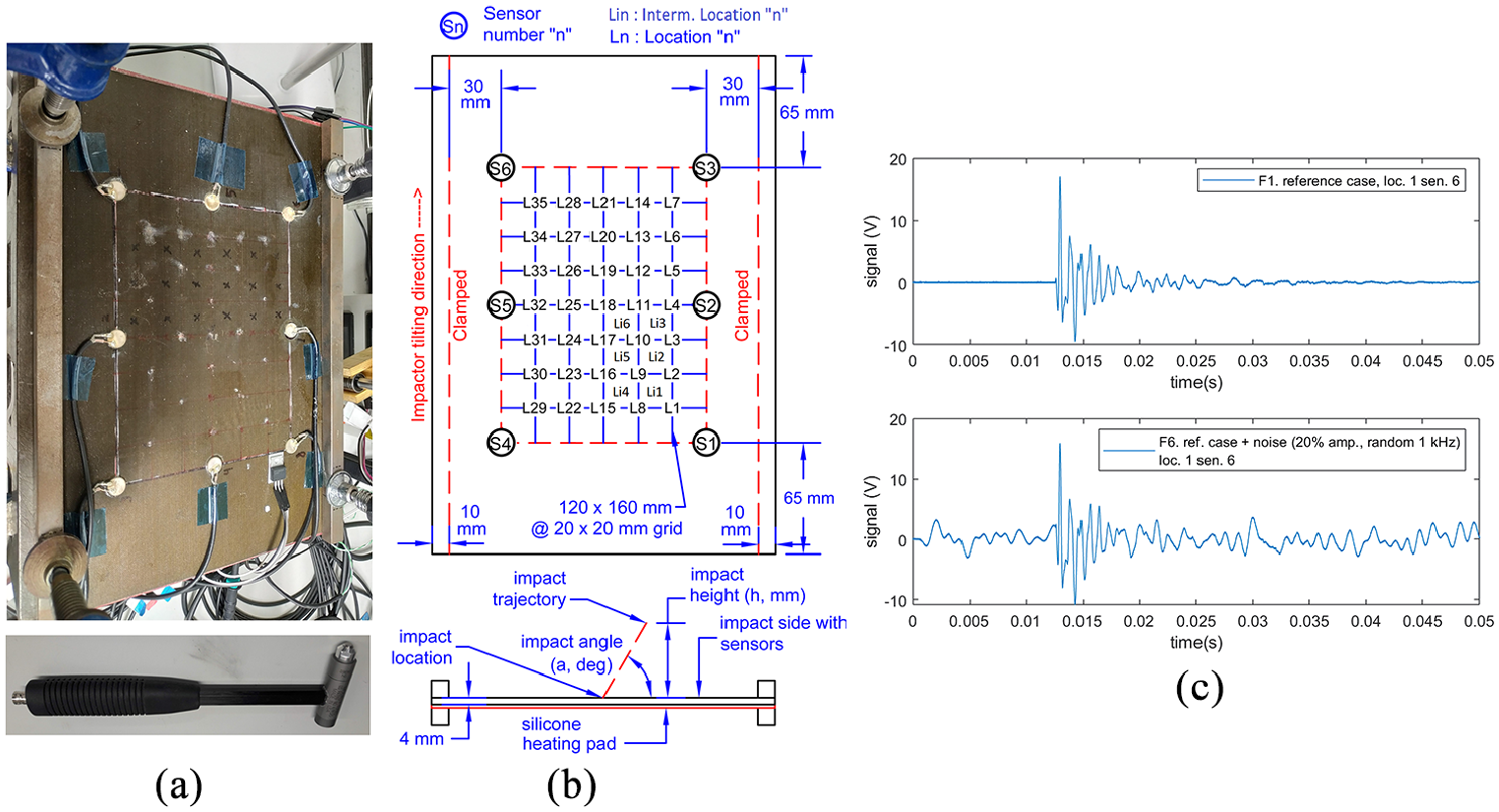
Flat panel experimental impact setup: (a) flat panel and impact hammer, (b) layout of flat panel and (c) example of impact signals.

Handheld impacts (with random angle and energy, ranging from 50 to 250 N maximum force) were imparted on two sensorised composite specimens, a simple flat (M21 T800s, (0/+45/−45/90/0/+45/−45/90)s layup) panel and a more complex stiffened (M21 T800s, (45/−45/0/0/90/0)s layup) panel, following the layout shown in Figures 1 and 2. The flat panel has a silicone heating mat underneath and a temperature control system to simulate increased temperatures (Figure 1). To simulate vibration noise, artificial 1 kHz random noise at 20% of the maximum recorded signal amplitude was generated through band filtering of white noise^5,13 and superimposed to the impact signals of the reference case (Figure 1(c)).

Figure 2.

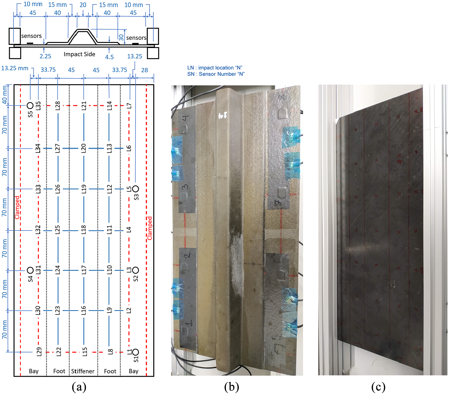
(a) Stiffened panel experimental impact setup. (b) Layout, stiffened panel bottom where the sensors are located. (c) Top side where the impacts are conducted.

Impact-induced Lamb wave signals were recorded through the attached PZT sensors on each plate (Figures 1 and 2), which are connected to an 8-channel PXI-5105 oscilloscope through 10x attenuation probes. Signals were recorded at 2 MS/s with a length of 100,000 sample points. As the force measurement from the impact hammer requires one oscilloscope channel, thus not all eight PZT sensors are used on each panel. For the flat panel, six sensors were used as shown in Figure 1, while only five sensors were used (Figure 2) on the stiffened panel due to damaged sensors from previous testing campaigns. All data processing was done using MathWorks MATLAB.

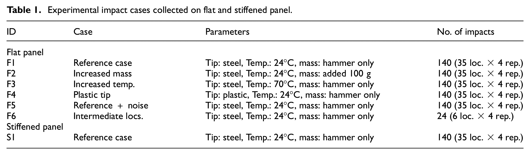
In total, data from six impact cases (F1–F6) representing parametric variations (reflecting simulated environmental and operational conditions) from a reference case (F1) were collected from the flat panel, while one case (S1) was collected from the stiffened panel as listed in Table 1. For each case, impacts were conducted at each location as shown in Figures 1 and 2 with four repetitions each, resulting in the total number of impacts shown in Table 1. None of the impacts generated damage on the panels. For the reference case of each panel (F1 and S1), an impact from each location (35 impacts) was used to build the reference database ⁵ of each plate for the impact location and force estimation algorithms, while the rest of the impact data was used as test data.

Table 1.

Experimental impact cases collected on flat and stiffened panel.

ID	Case	Parameters	No. of impacts
Flat panel
F1	Reference case	Tip: steel, Temp.: 24°C, mass: hammer only	140 (35 loc. × 4 rep.)
F2	Increased mass	Tip: steel, Temp.: 24°C, mass: added 100 g	140 (35 loc. × 4 rep.)
F3	Increased temp.	Tip: steel, Temp.: 70°C, mass: hammer only	140 (35 loc. × 4 rep.)
F4	Plastic tip	Tip: plastic, Temp.: 24°C, mass: hammer only	140 (35 loc. × 4 rep.)
F5	Reference + noise	Tip: steel, Temp.: 24°C, mass: hammer only	140 (35 loc. × 4 rep.)
F6	Intermediate locs.	Tip: steel, Temp.: 24°C, mass: hammer only	24 (6 loc. × 4 rep.)
Stiffened panel
S1	Reference case	Tip: steel, Temp.: 24°C, mass: hammer only	140 (35 loc. × 4 rep.)

For the purpose of impact localisation, the ToA difference of the Lamb wave signals from each sensor towards the earliest signal from the sensor set (as the actual impact event time is unknown) was chosen as the input feature. To mitigate the effect of the simulated vibration noise (case F5) in masking the start of the signal (Figure 1(c)), all signals were highpass filtered with a 2 kHz Butterworth IIR filter prior to ToA extraction. The ToA was then extracted using the normalised smoothed envelope threshold (NSET) method developed in Seno et al. ⁶ First, the signal was converted into its absolute values, then it was lowpass filtered with a 250 Hz IIR Butterworth filter. Afterwards, the amplitude of the signals from each sensor is normalised with respect to the largest amplitude in the set of sensors. The ToA was then taken when the resulting envelope passes a predetermined threshold (0.05 used here).

For maximum impact force estimation, the maximum absolute (MA) signal amplitude was used as the input feature. No highpass filtering was done beforehand even in the presence of simulated random vibration noise (case F5), as the maximum impact force estimation method developed in Seno and Aliabadi ¹³ has been shown to be robust towards the change in amplitude. The maximum measured impact force together with the MA signal amplitude at the reference database points (cases F1 and S1, Table 1) were used to calculate the force gradient for the maximum impact force estimation as will be explained in section ‘Force gradient method for deterministic maximum impact force estimation’.

To estimate impact location and maximum force, the features ToA and G_ma are extracted from an impact on each location (35 × 1 impacts, Table 1) of the reference cases (F1 for the flat panel and S1 for the stiffened panel, Table 1) and used as the reference database of the algorithms (each panel has its own specific database). The features ToA and A_ma from the other impacts of the reference cases (F1 and S1, 35 × 3, see Table 1) and the other cases (F2–F6, see Table 1) were used as inputs for testing.

Benchmark impact location and maximum force estimation methods

The benchmark data-driven impact location method (reference database method ⁵ ) and maximum impact force estimation method (force gradient method ¹³ ) were taken from previous studies which have proven to be accurate and robust for simple structures under simulated environmental and operational conditions using minimum initial data.

Reference database method for deterministic impact location estimation

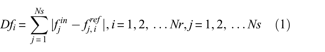
The reference database method is essentially a pattern matching method where the impact location estimate is obtained based on the similarity of features (ToA differences used in this study) of the incoming signal to that of signal features known for specific locations in a reference database (obtained from the reference impact cases F1 and S1).^5,9 To do so, first, the absolute difference (Df_i) between the incoming signal’s features (fⁱⁿ) and the known features in the reference database (f^ref) is calculated, as shown in equation (1), for all sensors (Ns) and all reference database points (Nr). The location estimate is then taken as the location of the database point with minimum difference (Df)

$$D{f}_i=\sum _{j=1}^{\mathrm{Ns}}|f_j^{\mathrm{in}}-f_{j,i}^{\mathrm{ref}}|,i=1,2,\dots \mathrm{Nr},j=1,2,\dots \mathrm{Ns}$$

(1)

Using the above definition, the location estimation is limited to points that exist in the reference database. To achieve a more thorough coverage of locations without requiring too many initial data points to build the reference database, cubic spline interpolation is used (selected from MATLAB library of interpolation functions that can handle non-uniform grids as used in the stiffened panel) to approximate the features at locations between the reference database points (two points between reference points are interpolated in this study).

To increase the robustness of the final estimate, rather than calculating a single difference value for each reference point (Df_i), all the features available are used at once. Multiple values are generated by creating different combinations of features used, for example, if there are six sensors, then using combinations of five yields 12345, 12346, 12456, and so on, resulting in six feature sets and location estimates in the end. The location estimates are subsequently averaged to obtain the final estimate. Here, combinations of five (out of six) ToA difference values for the flat panel and four (out of five) for the stiffened panel were used.

Force gradient method for deterministic maximum impact force estimation

The force gradient method is based on the linear relation between the maximum impact force (F_max) and the MA signal amplitude (A_ma), as shown in equation (2), which is a faster and simpler way of estimating the maximum impact force than reconstructing the whole impact force history. ¹³ Once the gradient (G_ma) is known (i.e. calculated from the pair of F_max and A_ma from the impact location of the reference cases, F1 and S1, Table 1), it is possible to estimate the maximum impact force from signals with varying amplitude. The gradient of this linear relation has been found to be constant for most simulated environmental and operational conditions (except very soft impactor materials, e.g. silicone) and low (non-damaging impacts) or high (damaging) energy impacts, but it is location (x, y) and temperature (T) dependent ¹³

$$F_{\max }(x,y)=G_{\mathrm{MA}}(x,y)A_{\mathrm{MA}}(x,y)(1-\alpha [T-T_{\mathrm{ref}}])$$

(2)

Lamb wave amplitude is known to have an inverse linear relation with temperature (T),^13,26 thus it is necessary to apply a compensation factor (α) relative to a certain reference temperature (T_ref). For the panel used in this study, the linear relation has been determined in a previous study (α = −0.0026, T_ref = 24°C ¹³ ) and the results were used here, mostly for the increased temperature case (case F3). As the gradient also depends on location, for the reference database, the measured maximum impact force and MA signal amplitude from the reference case (F1 and S1) were used to obtain the gradient value at each location. As each sensor can give an estimate, the final force estimate was taken from the average from all sensors.

Similar to the localisation method described in section ‘Reference database method for deterministic impact location estimation’, cubic spline interpolation is used to approximate the gradient values at locations outside of the original reference points. The gradient values are location-dependent; therefore, to obtain the appropriate value, the impact location must be known beforehand. Here, the location estimate results from the localisation algorithm described in section ‘Reference database method for deterministic impact location estimation’ were used. This approach has a disadvantage, as the error of the location estimation is carried over to the estimated maximum force gradient values. Figure 3 illustrates how the deterministic localisation and force estimation methods are combined.

Figure 3.

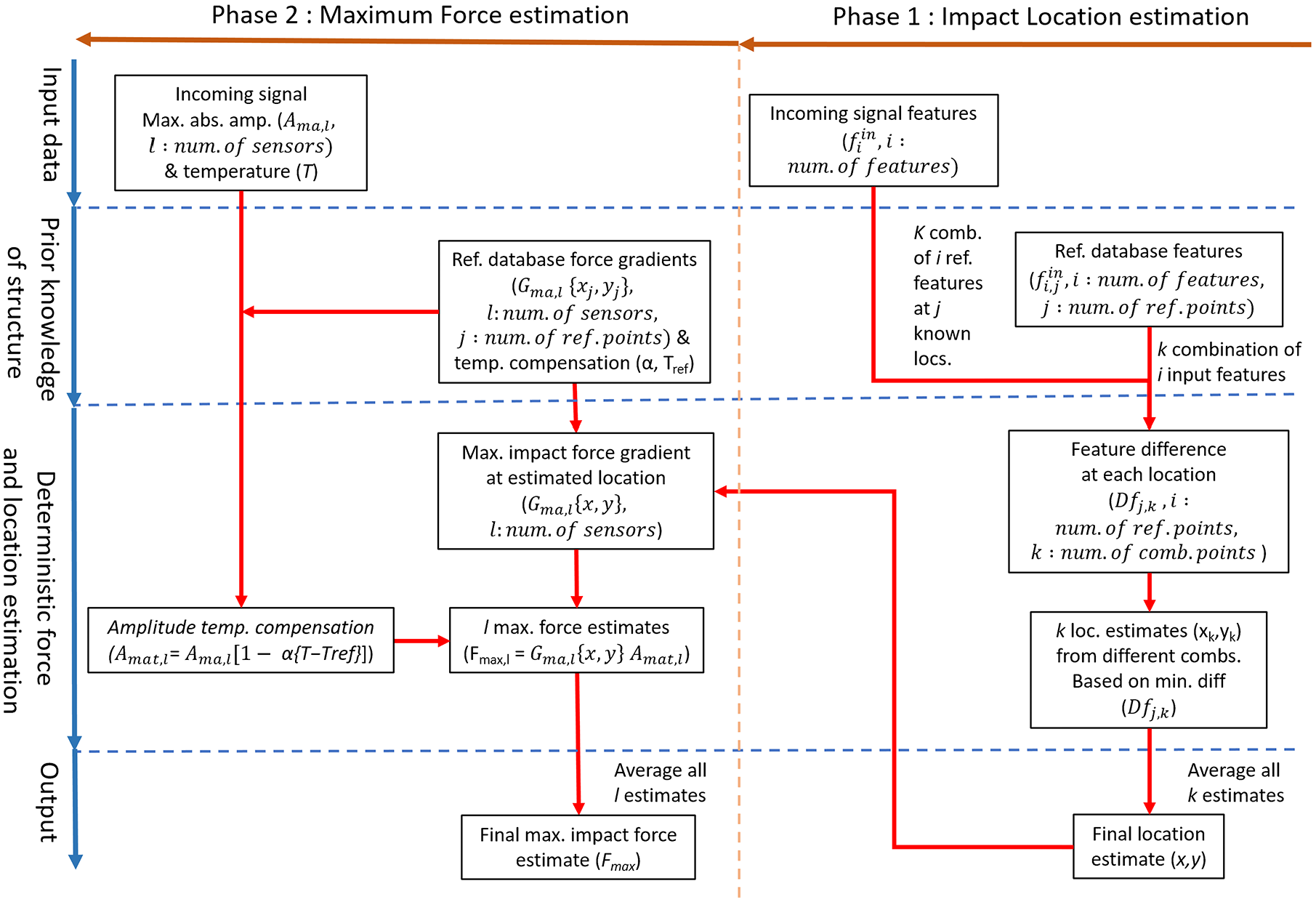
Diagram of benchmark deterministic impact location and maximum force estimation algorithm.

Uncertainty quantification method for impact location and maximum force estimation

To allow for estimates of the uncertainties obtained using the benchmark location and maximum force estimation algorithms be incorporated in the analysis, a novel application of the kriging technique ²⁵ is presented in this section. Originally, kriging was used for spatial interpolation of geostatistical data; however, here we propose to modify it for statistical pattern matching between the incoming impact features and the features of the reference database points to estimate the location and maximum force of impacts. Using the proposed method, it is possible to not only obtain an estimate but also the uncertainty of the estimate based on the relationship between data points used in the reference database. ²⁵

Kriging method for spatial interpolation

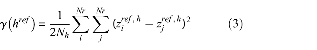
Kriging was originally developed for spatial interpolation of geostatistical data, using the spatial correlation between existing reference data points to determine weights for use in a linear combination of the available data points to determine the interpolated value. ²⁵ The spatial correlation between data points may be expressed in many forms, ²⁵ but one of the most widely used is the semivariance (γ(h^ref)) between data points, as shown in equation (3). Semivariance values (γ(h^ref)) for a certain distance (h^ref) are calculated for each data point pair combination that is separated by that distance (z_i^{ref, h}, z_j^{ref, h}) and are averaged based on the number of data pairs that share the same distance (N_h). This is done for all the reference data points (Nr) in their possible pair combinations. It quantifies how the variance between data points changes (usually increasing) as their respective distance (h^ref) increases (or how the correlation is higher between closer data points). As the distance (h^ref) between data pairs may not always be exactly the same, they are usually grouped into bins (20 bins used in this study) to allow averaging. ²⁵ Afterwards, a semivariance function (γ^fc(h)) is fitted to the discreet empirical semivariance values (γ(h^ref)) to allow approximation of the semivariance at a continuous distance range (h) ²⁵

$$\gamma \left(h^{\mathrm{ref}}\right)=\frac{1}{2N_h}\sum _i^{\mathrm{Nr}}\sum _j^{\mathrm{Nr}}(z_i^{\mathrm{ref},h}-z_j^{\mathrm{ref},h}{)}^2$$

(3)

To estimate the value of an interpolated point, first, the distance between the point and the existing reference data points (hⁱⁿ) is calculated. Afterwards, using the previously obtained semivariance function (γ^fc(h)), the approximate semivariance values for the reference (γ^fc(h^ref)) and interpolated (γ^fc(hⁱⁿ)) data point pairs are calculated based on their respective distances (h^ref and hⁱⁿ). Equation (4) is then solved (I_j is a column vector of 1’s with j number of rows) to obtain the kriging weights (w_i) and the Lagrange parameter (μ)

$$\left[\begin{array}{cc}{\gamma }_{\mathrm{ij}}^{\mathrm{fc}}\left(h^{\mathrm{ref}}\right)\hfill & I_i\hfill \\ \multicolumn{1}{c}{I_j^T}& 0\hfill \end{array}\right]\left[\begin{array}{c}{w}_i\hfill \\ \multicolumn{1}{c}{\mu }\end{array}\right]=\left[\begin{array}{c}{\gamma }_i^{\mathrm{fc}}\left(h^{\mathrm{in}}\right)\hfill \\ \multicolumn{1}{c}{1}\end{array}\right]i,j=1,2,3\dots .\mathrm{Nr}$$

(4)

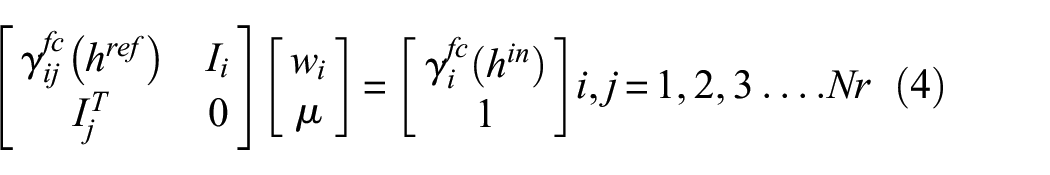
With the obtained values, the interpolated value (z_est) and uncertainty (in the form of a standard deviation, σ^est, from the interpolated value) can be calculated from equation (5). As the semivariance values are always positive, to ensure that the estimated uncertainty is real-valued, the kriging weights and Lagrange parameter need to be positive-valued. Thus, a non-negative constrained linear least square solver (MATLAB lsqnonneg) is used to solve equation (4)

$$z^{\mathrm{est}}=\sum _{i=1}^{\mathrm{Nr}}{w}_i{z}_i^{\mathrm{ref}},{\sigma }^{\mathrm{est}}=\sqrt{\mu +\sum _{i=1}^{\mathrm{Nr}}{w}_i{\gamma }_i^{\mathrm{in}}\left(h^{\mathrm{in}}\right)}$$

(5)

Kriging application for impact location and maximum force estimation

In section ‘Benchmark impact location and maximum force estimation methods’, it was shown that the impact location is determined by simply choosing the point in the reference database that has the minimum difference in features compared to the incoming impact signal. ⁵ In turn, the maximum impact force gradient is then taken as the value known for the said reference point. This way, there is a significant amount of information discarded as only the information from a single database point is used at the end. Here, we propose to substitute this criterion with the kriging technique which can interpolate the location and also the maximum impact force gradient using the information from all of the reference database points while also estimating the uncertainty.

Contrary to the original application of kriging as shown in section ‘Kriging method for spatial interpolation’, in our case, the value at the point of interest (in the form of the incoming impact signal features) is already known, and what is to be estimated instead is the location of the point. Here, we propose to substitute the actual spatial distance between data points, (which is the difference in spatial coordinates) with the difference in feature values (calculated by the L2 norm of the difference vector). Thus, here data points are grouped not based on spatial closeness but by the similarity of their features. The values to be interpolated are then the actual spatial coordinates (x, y) of the data point locations and the respective maximum impact force gradients (G_ma(x, y)). Thus, using the features of the incoming impact signal, it is possible to estimate the location of the impact event and the maximum impact force.

Here, the L2 norm of the vector of ToA difference between the reference and interpolated data points was used to calculate their respective ‘distances’ (between reference data points, h^ref, and also between reference and input points, hⁱⁿ). The semivariance (γ(h^ref)) of the reference database points was calculated for the estimated variables (z: x, y, G_ma(x, y)) of each sensor using equation (3) as shown in Figure 4. A linear function (γ^fc(h) = G_γ h) was then fit for all estimated variables to obtain the approximate semivariance values for equation (4). Then, equation (4) was solved to obtain the kriging weights and Lagrange parameter to calculate the final estimate and uncertainty of the impact location coordinates and maximum impact force gradients for each sensor using equation (5). A normal probability distribution function (P) was then formed using the estimate (z^est, as mean) and standard deviation (σ^est) for all estimated variables.

Figure 4.

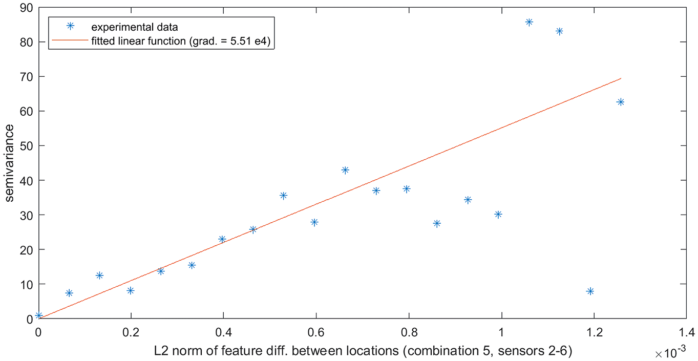
Semivariance of Sensor 5 maximum impact force gradient versus L2 norm of ToA difference from Sensors 2–6 (combination 5) for the stiffened panel.

Following the benchmark localisation method in section ‘Reference database method for deterministic impact location estimation’, the ToA difference values were also used in combinations rather than all at once, resulting in multiple estimate distributions of the impact location coordinates and the maximum impact force gradients. For each of these combinations, there is a further set of maximum impact force gradients from each sensor. The maximum impact force estimate distributions are obtained by multiplying the obtained gradient distributions with the signal amplitude for each sensor, following equation (2).

It must be noted that using this approach, the maximum impact force gradients (G_ma(x, y)) are determined independently from the estimated location unlike in the benchmark method (section ‘Benchmark impact location and maximum force estimation methods’, Figure 3), thus the localisation error is not imposed on the maximum impact force estimation. In addition, the kriging method is able to interpolate values between the reference data points due to the fitted semivariance functions, thus there is no need for the cubic interpolation done in the benchmark method.

Fusion of impact location and maximum force distributions

As the kriging method given in section ‘Kriging application for impact location and maximum force estimation’ results in multiple estimate distributions for each output variable, here methods to fuse them together are outlined. The first alternative is to simply take the mean of the estimates (as is done with the benchmark method) to obtain a wider and more conservative final estimate distribution as shown in Figure 5. To ensure that the total probability of the distribution is unity, it is divided by the area under the mean probability density function.

Figure 5.

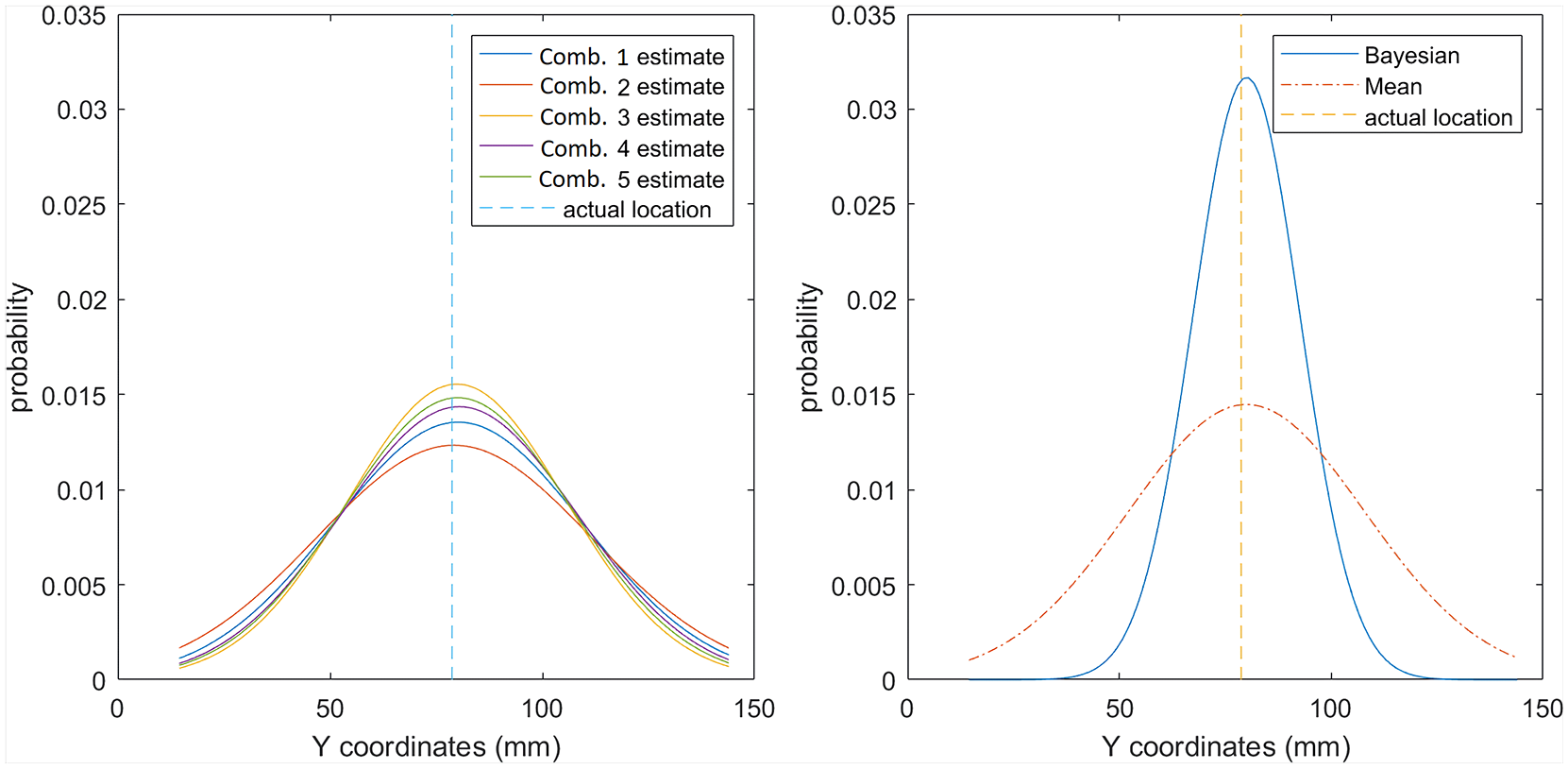
Estimate distributions for Y coordinate from sensor combinations 1–5 (left) and fused final estimates using mean and Bayesian updating (right).

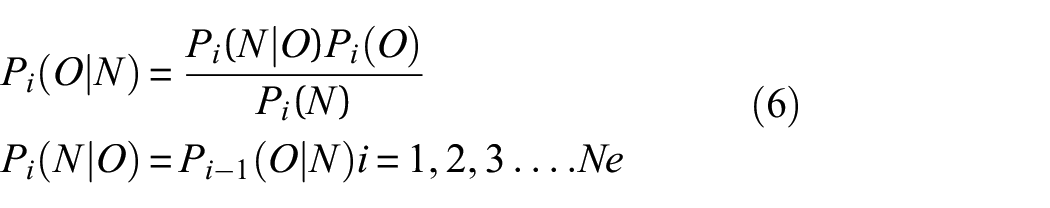
Another method is to apply Bayesian updating, ⁸ treating multiple estimates as new information that can update prior estimates. It starts with an initial/prior assumption of the estimated variables (P(O)), which in this study was taken as a uniform distribution as there was no initial knowledge of their values. ⁸ The estimates from kriging were then used to ‘update’ (P(N|O)) our prior assumption to obtain a more ‘informed’ estimate (P(O|N)) as shown in equation (6). Here P(N) is a normalising factor (obtained from the area under the distribution of P(N|O) P(O) to ensure that the total probability of P(O|N) is unity. The informed estimate (P(O|N)) then becomes the new prior (P(O)) and is updated with the next available estimate (P(N|O)). This goes on until all of the available estimate distributions (Ne) have been used to obtain the final estimate distribution. This method results in a more narrow final estimate distribution compared to the original data (Figure 5) as the confidence of the estimation increases when updated with new information

$$\begin{array}{c}{P}_i(O|N)=\frac{P_i(N|O)P_i\left(O\right)}{P_i(N)}\hfill \\ P_i(N|O)=P_{i-1}(O|N)i=1,2,3\dots .\mathrm{Ne}\hfill \end{array}$$

(6)

As stated in section ‘Introduction’, the estimated range must be wide enough to ensure that the actual value reliably lies within the bounds of the distribution while at the same time must be narrow enough to give an estimate that is as precise as possible. Both the mean and Bayesian approaches have different characteristics and are thus both tested to compare their performance with the test data. For the maximum impact force, as there are multiple estimates not only from multiple sensors but also from the multiple feature combinations, there are two stages of fusion. Here both the mean and Bayesian approach were tested for both stages, and a third combination where the estimates from all sensors are first fused using the mean approach and the resulting estimates is finally fused using the Bayesian approach. Figure 6 shows the outline of the proposed kriging method accompanied by uncertainty fusion for both impact location and maximum force estimation.

Figure 6.

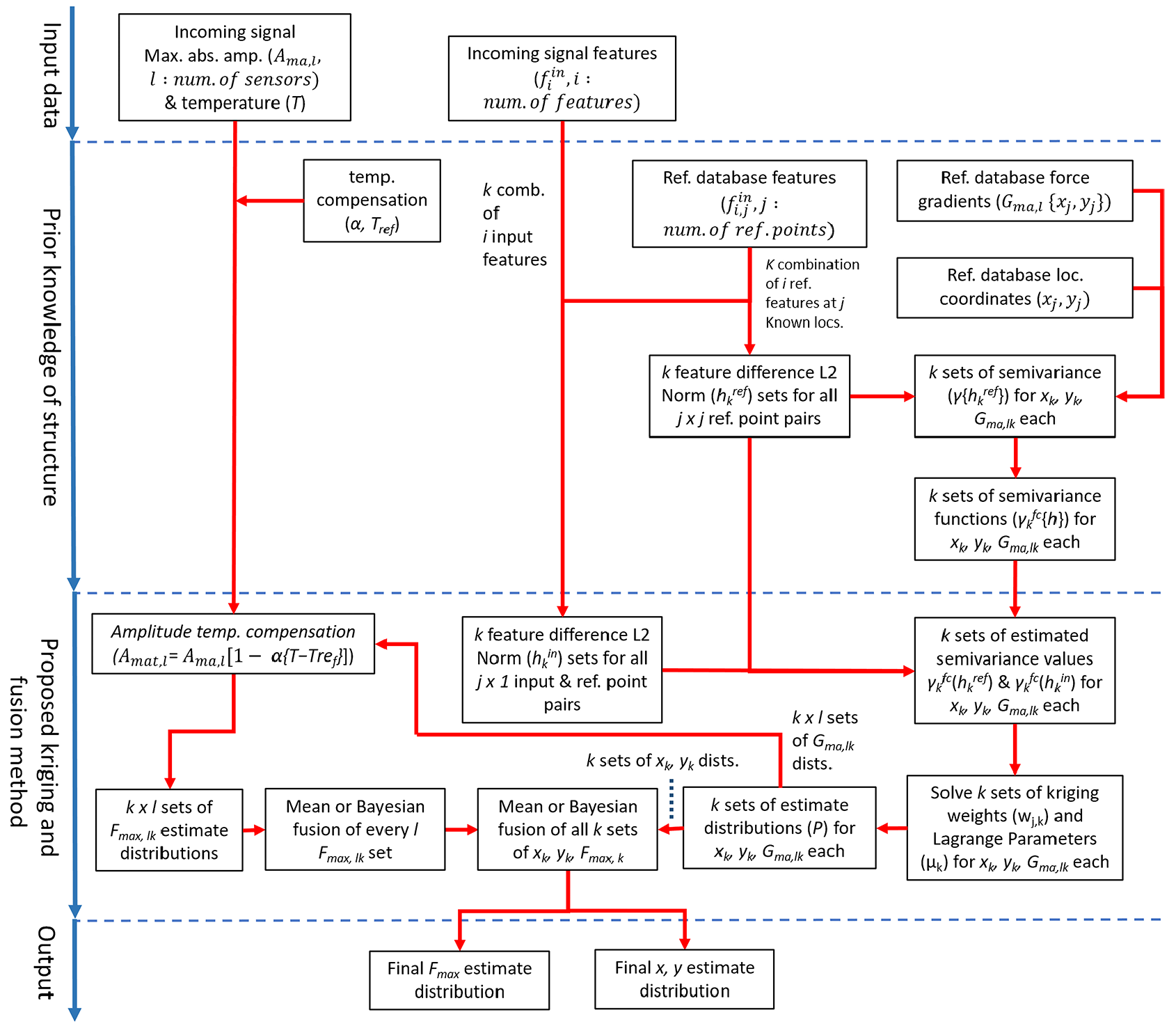
Diagram of proposed stochastic impact location and maximum force estimation algorithm.

Once the final distribution has been obtained, the upper and lower bound of the estimate range is determined within the 95% confidence interval of the distribution. For the impact location, an oval area is drawn around the estimated coordinates (x^est, y^est) using the estimate range of the x and y coordinates as the semi-major axes to mark the area at which there is 95% confidence that the impact location is located within.

Performance evaluation and comparison of benchmark and proposed methods

To evaluate and compare the performance of the proposed methods against the benchmark methods, the metrics used to measure the accuracy of the estimates are defined here. To compare the deterministic accuracy of both methods directly, the error of the estimated values from the benchmark and proposed methods towards the actual values for each test impact in Table 1 were compared.

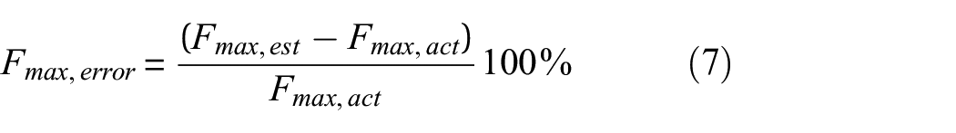
For maximum impact force, the error in estimation (F_max.error) is the difference between the estimate (F_{max, est}) from either algorithm towards the actual value (F_max,act). As the maximum impact force is random (ranging from 50 to 250 N), the error was taken as percentage towards the actual value as shown in equation (7). To summarise the error for a whole impact case, the mean (F_{max, mean}) and standard deviation (F_max,std) of the maximum force error for all impacts in the said case were calculated ¹³

$$F_{max,error}=\frac{(F_{max,est}-F_{max,act})}{F_{max,act}}100\%$$

(7)

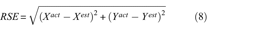
For impact location, the error of the estimated location (x^est,y^est) towards the actual location (x^act,y^act) was calculated from the root square error (RSE) as shown in equation (8). To summarise the localisation errors (RSE) for an impact case (Table 1), a gamma distribution was then fit on the RSE values and the 90th percentile of the cumulative distribution function (RSE_90th) was then taken as the range from the actual location that encompasses 90% of the localisation errors^5,6

$$\mathrm{RSE}=\sqrt{{(X^{\mathrm{act}}-X^{\mathrm{est}})}^2+{(Y^{\mathrm{act}}-Y^{\mathrm{est}})}^2}$$

(8)

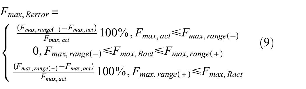
To evaluate the reliability of the uncertainty estimates, the error of the estimate range (upper and lower bounds based on 95% confidence interval) for both the maximum impact force and location was calculated. For the maximum impact force range (F_{max, range(−)} to F_{max, range(+)}), the estimate range error (F_max,Rerror) is defined to be 0 when the actual force (_Fmax,act) is within the estimated range. However, when the actual force is outside of the estimated range, then the error is calculated similar to the deterministic error in equation (7), but relative to the nearest bound (upper or lower) as shown in equation (9). To summarise the estimated range error for a whole impact case, the mean (F_{max, Rmean}) and standard deviation (F_max,Rstd) for all the impacts in the said case were calculated as is done with the deterministic errors

$$F_{max,Rerror}=\{\begin{array}{c}\frac{(F_{max,range(-)}-F_{max,act})}{F_{max,act}}100\%,F_{max,act}\le F_{max,range(-)}\\ 0,F_{max,range(-)}\le F_{max,Ract}\le F_{max,range(+)}\\ \frac{(F_{max,range(+)}-F_{max,act})}{F_{max,act}}100\%,F_{max,range(+)}\le F_{max,Ract}\end{array}$$

(9)

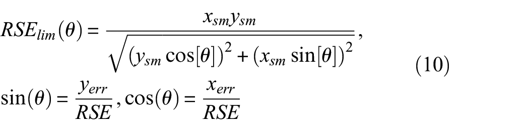
For impact location, the location estimate range was defined as an oval area around the estimated location (x^est,y^est) with the upper (x_range(+), y_range(+)) and lower bounds (x_range(−), y_range(−)) of the coordinates as the semi-major axes (x_sm,y_sm as the distance from x^est,y^est to bounds). The radius of the oval area (RSE_lim) at any angle (θ) is given by equation (10). The coordinates of the actual impact location relative to the estimated location (in other words the location error, x_err, y_err) can also be defined in polar coordinates (RSE, θ). When the radius of the location error (RSE) is smaller than the radius of the oval area limit (RSE_lim) for a given angle, the actual location (x, y) is located inside the estimated oval range and thus the error is 0. When the radius of the location error is larger than the radius of the oval area limit, the actual impact location is outside the estimate range and the error of the oval range is calculated as RSE_range = RSE − RSE_lim. To summarise the localisation error for an impact case, a gamma distribution is fitted to the range error and the 90th percentile value (RSE_R90th) of the cumulative distribution function is taken as done for the deterministic location error

$$\begin{array}{c}\mathrm{RS}{E}_{\lim }\left(\theta \right)=\frac{x_{\mathrm{sm}}{y}_{\mathrm{sm}}}{\sqrt{{\left(y_{\mathrm{sm}}\cos \left[\theta \right]\right)}^2+{\left(x_{\mathrm{sm}}\sin \left[\theta \right]\right)}^2}},\hfill \\ \sin \left(\theta \right)=\frac{y_{\mathrm{err}}}{\mathrm{RSE}},\cos \left(\theta \right)=\frac{x_{\mathrm{err}}}{\mathrm{RSE}}\hfill \end{array}$$

(10)

Results

Table 2 shows the comparison of the deterministic impact location estimation for both the benchmark and the proposed kriging method (using mean (K+M) and Bayesian (K+B) fusion methods). It can be seen that all three methods are considerably accurate for all cases tested (F1–F6 and S1) and there is no significant difference between the accuracy of the deterministic location estimates between these methods.

Table 2.

Benchmark versus proposed kriging method deterministic location estimation.

Impact case	BM RSE90th (mm)	K + B RSE90th (mm)	K + M RSE90th (mm)
Flat panel
F1. steel hammer, ref. case	5.1	5.9	5.9
F2. steel hammer, incr. mass	6.7	6.9	7
F3. steel hammer, incr. temp.	6.3	6.7	6.5
F4. plastic hammer	7.6	8	7.9
F5. steel hammer, + noise	5.2	6	5.9
F6. steel hammer, interm. loc.	8.6	7.3	7.4
Stiffened panel
S1. steel hammer, ref. case	25.3	25.7	26.5

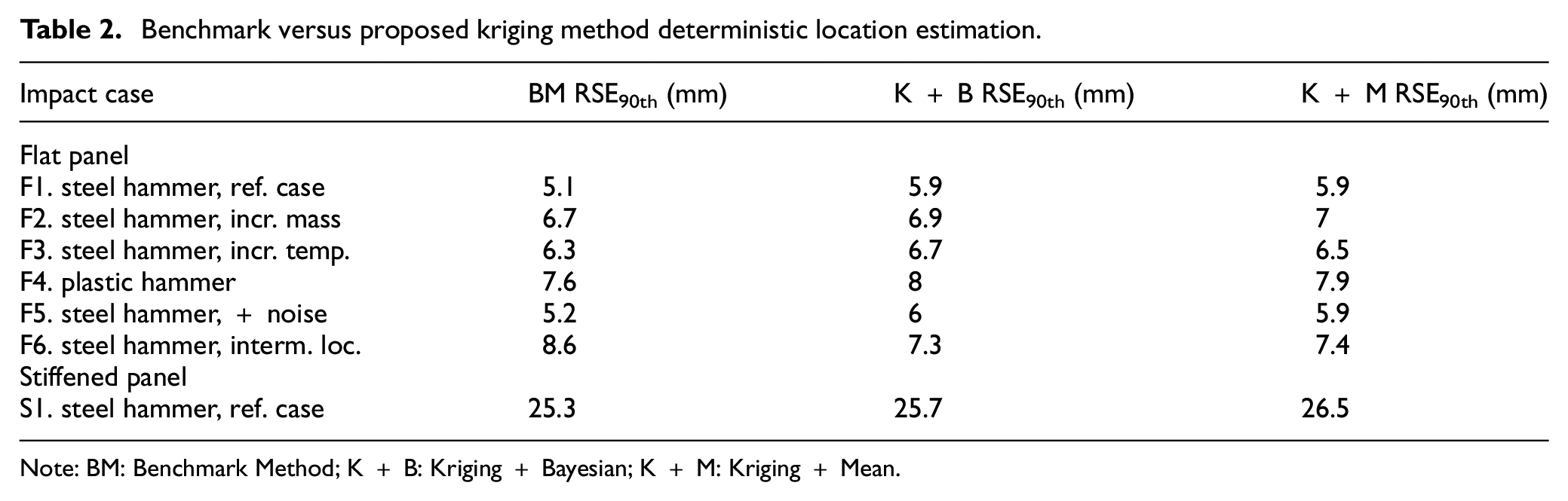
Note: BM: Benchmark Method; K + B: Kriging + Bayesian; K + M: Kriging + Mean.

Similarly, comparing the deterministic maximum impact force estimation (Table 3) of the benchmark and proposed kriging method (with mean–mean (K+M+M), Bayesian–Bayesian (K+B+B) and mean–Bayesian (K+M+B) fusion methods), it was found that all methods were considerably accurate for all cases tested (case F1–F6) apart from the stiffened panel (S1). This is due to the stiffened panel having more spatial variation of the maximum impact force gradient (and thus higher sensitivity) due to the stiffness difference from each stiffener zone (Figure 2). It is worth noting that as the benchmark method utilises the estimate of the impact location, the localisation errors can introduce inaccuracies in the force estimation. This is apparent in the lower accuracy of the benchmark force estimates compared to the proposed kriging method (which determines the maximum force gradient independent of localisation) for the stiffened panel (S1).

Table 3.

Benchmark versus proposed kriging method deterministic impact force estimation.

Impact case	BM avg. Fmax, error (%)	K+B+B avg. Fmax, error (%)	K+M+M avg. Fmax, error (%)	K+M+B avg. Fmax, error (%)
Flat panel
F1. steel hammer, ref. case	0.2±3.8	0±4	−0.3±4	−0.3±4
F2. steel hammer, incr. mass	−4.5±4.5	−6.8±4.5	−7.3±4.3	−7.3±4.3
F3. steel hammer, incr. temp.	9.3±4.4	9.7±5.1	8±5.1	8.1±5.2
F4. plastic hammer	12±4.4	10.7±4.5	10±5	10±5
F5. steel hammer,+noise	0.9±4.7	0.5±5.1	0.2±5.5	0.2±5.4
F6. steel hammer, interm. loc.	7.1±8	4.4±4.3	3.8±4.2	3.8±4.2
Stiffened panel
S1. steel hammer, ref. case	8±17.5	5.5±15.9	3.7±16.3	4.2±16.6

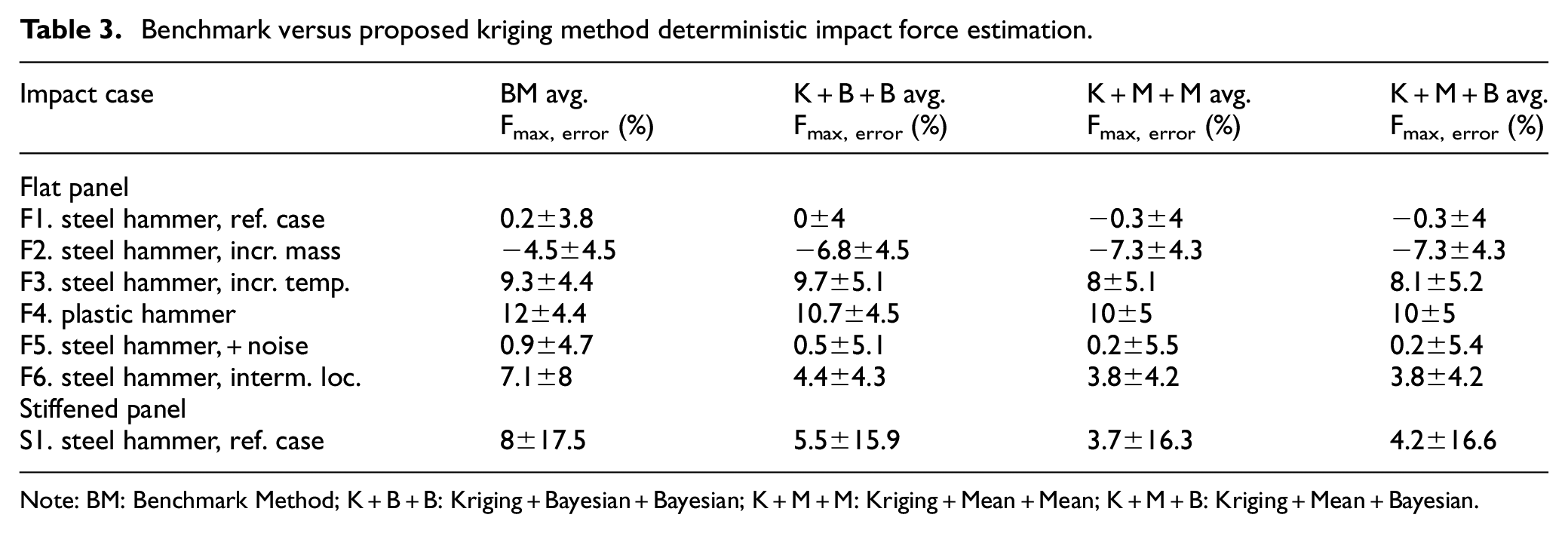
Note: BM: Benchmark Method; K+B+B: Kriging+Bayesian+Bayesian; K+M+M: Kriging+Mean+Mean; K+M+B: Kriging+Mean+Bayesian.

Although the deterministic estimates for both impact location and maximum force are mostly accurate, some level of error exists from the various sources of uncertainty that cannot be captured deterministically, especially as shown by the maximum impact force estimates of the stiffened panel (S1, Table 3). Tables 4 and 5 show the estimated accuracy for the stochastic approach using the proposed kriging method to define estimates in terms of a range (instead of a deterministic point) encompassing the estimated degree of uncertainty. For impact location (Table 4), it can be seen that both kriging methods (with mean (K+M) and Bayesian (K+B) fusion methods) have very high reliability, with all actual impact locations being situated within the estimated uncertainty range (cases F1–F6) or being only slightly outside (case S1). Looking at the uncertainty range, it can be seen that using the Bayesian updating method, the estimated location coordinates (x, y) had significantly smaller uncertainty ranges (more than 2x) compared to the mean fusion method, with only a small trade-off in accuracy. Thus, the Bayesian method is the better fusion method for location estimation as it allows for reliable and precise location estimation.

Table 4.

Evaluation of proposed kriging method location uncertainty estimation.

Impact case		K+B RSER90th (mm)	K+M RSER90th (mm)	K+B avg. x unc. (mm)	K+B avg. y unc. (mm)	K+M avg. x unc. (mm)	K+M avg. y unc. (mm)
Flat panel
F1	steel hammer, ref. case	0	0	22.4±5.1	14.5±3.3	50.6±11.4	32.9±7.4
F2	steel hammer, incr. mass	0	0	24.1±4.7	15.7±3	54.6±10.2	35.6±6.7
F3	steel hammer, incr. temp.	0	0	28.9±7.1	18.7±4.6	65.6±16.5	42.6±10.5
F4	plastic hammer	0	0	25.8±6.1	16.8±4	58.5±13.9	38.2±9
F5	steel hammer,+noise	0	0	22.3±5.1	14.5±3.3	50.6±11.5	33±7.4
F6	steel hammer, interm. loc.	0	0	31±3.6	20±2.3	69.2±7.9	45.1±5.1
Stiffened panel
S1	steel hammer, ref. case	1.3	0	74.2±18.4	29.5±7.3	159.5±40.4	64.7±16.5

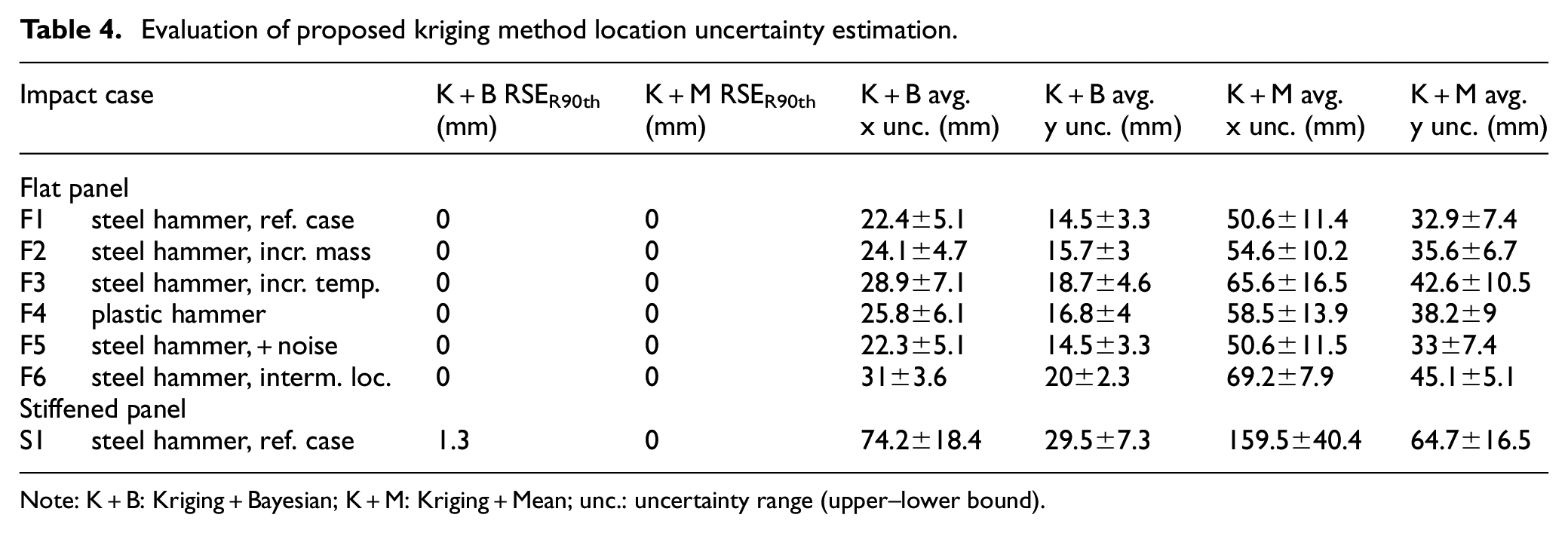
Note: K+B: Kriging+Bayesian; K+M: Kriging+Mean; unc.: uncertainty range (upper–lower bound).

Table 5.

Evaluation of proposed kriging method impact force uncertainty estimation.

Impact case		K+B+B Fmax, Rerror (%)	K+M+M Fmax, Rerror (%)	K+M+B Fmax, Rerror (%)	K+B+B avg. Fmax unc. (N)	K+M+M avg. Fmax unc. (N)	K+M+B avg. Fmax unc. (N)
Flat Panel
F1	steel hammer, ref. case	−0.3±1.7	0±0	0±0.2	12.1±3.8	82.1±31.2	28±8.2
F2	steel hammer, incr. mass	−4.1±3.7	0±0	−1.3±2	12.5±3	102.6±39.7	33.4±9.5
F3	steel hammer, incr. temp.	5.5±3.9	0±0	0.8±1.7	18.9±6	153.6±66.7	47±13.9
F4	plastic hammer	6.8±3.7	0±0	1.9±2.5	16.4±5.7	125.5±51.3	40.8±11.7
F5	steel hammer,+noise	0.1±2.7	0±0	0±0.6	12.2±3.8	89.8±30.7	32.2±9.2
F6	steel hammer, interm. loc.	1.6±2.4	0±0	0.1±0.3	17.3±2.6	119.9±16.9	43.7±6
Stiffened panel
S1	steel hammer, ref. case	2.4±10.3	−0.1±0.7	0.7±5.3	20.6±8.5	142.6±68.9	51.6±29.6

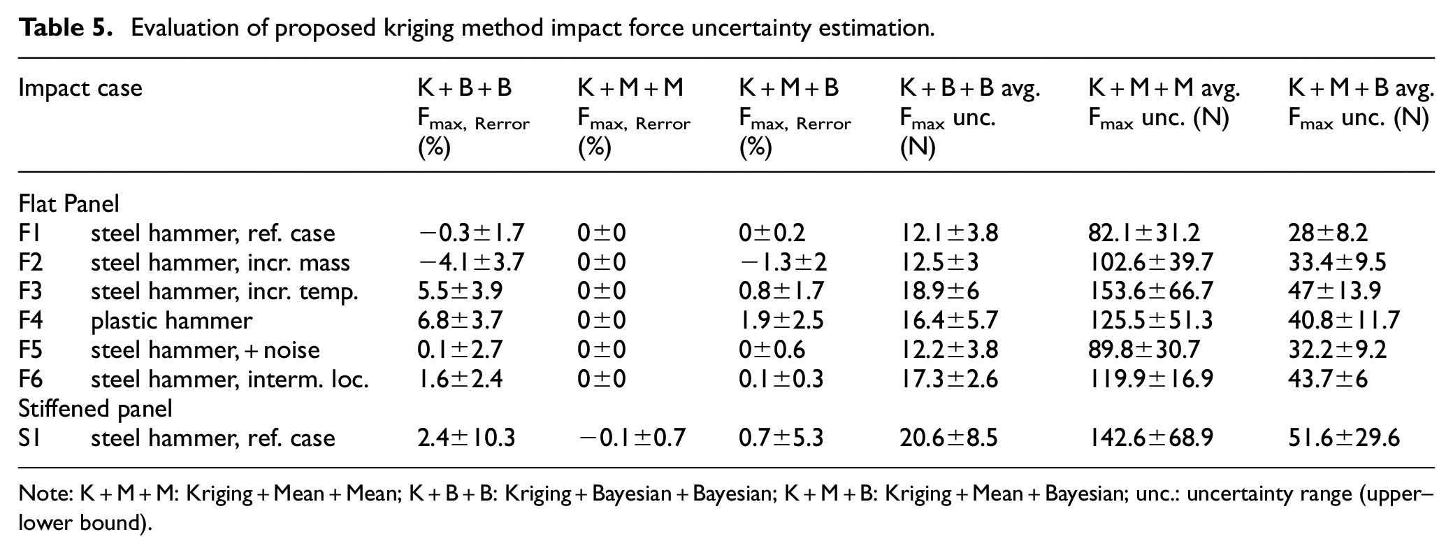
Note: K+M+M: Kriging+Mean+Mean; K+B+B: Kriging+Bayesian+Bayesian; K+M+B: Kriging+Mean+Bayesian; unc.: uncertainty range (upper–lower bound).

For maximum impact force estimation, Table 5 shows the estimation accuracy using the proposed kriging method accompanied by three different fusion methods (Bayesian–Bayesian (K+B+B), mean–mean (K+M+M) and mean–Bayesian (K+M+B)). Using the Bayesian–Bayesian fusion method, the estimated uncertainty range is very narrow up to the level where it becomes inaccurate as some of the actual maximum force values are not encompassed in the estimated range. This is similar to what was encountered by Morse et al. ⁸ when using successive Bayesian updating or Kalman filters for estimating impact location. This is due to the fact that what is fused are estimates and not actual measurements, thus it will not necessarily converge to the actual measurement (location or force).

However, using the mean–mean fusion method results in a very reliable (most actual values encompassed in estimated range) but very wide (up to 6x wider than the Bayesian–Bayesian method) and imprecise uncertainty range which may not be useful for impact severity assessment. This is similar to what is found from other ‘conservative’ methods, such as the bounded uncertainty approach, where the uncertainty distribution is reduced to a bounded range. ¹⁵ Using a combined mean–Bayesian method, a balance of good reliability and uncertainty range precision is achieved, making it more reliable than the Bayesian–Bayesian approach and more precise than the mean–mean approach. The proposed stochastic approach gives a much higher reliability of maximum impact force estimation compared to the deterministic method, especially for cases, such as the stiffened panel (S1) which is sensitive and difficult to estimate deterministically.

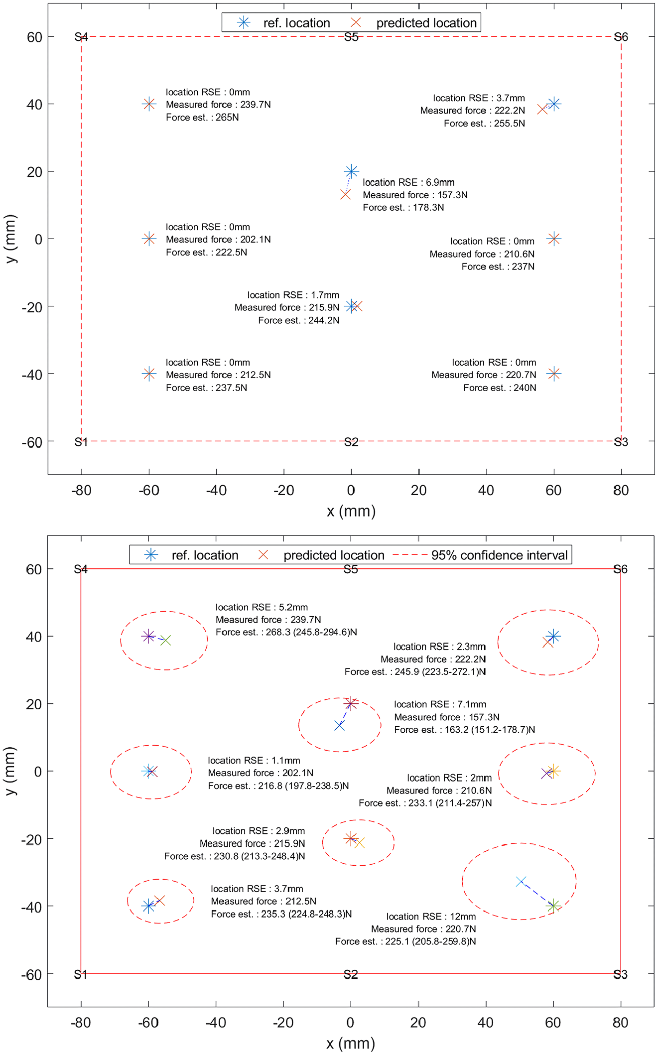
Figures 7 and 8 illustrate an example of the impact location and maximum force estimation using the benchmark and proposed kriging method (K+B for location and K+M+B for impact force). It can be seen that although the deterministic method is quite accurate, there is some degree of inaccuracy stemming from various sources of uncertainty, more so in some cases (such as in location 7 (Figure 8), bottom left of the stiffened panel (S1)) than others. However, the proposed kriging method is able to reliably estimate the uncertainty of the impact location and maximum force estimation (all actual locations and maximum impact force encompassed in estimated range), giving a more robust output for users to locate and assess the severity of an impact event.

Figure 7.

Example of location and maximum impact force estimation for plastic hammer tip (case F4) impacts on the flat panel using the benchmark deterministic method (top) and the proposed kriging stochastic method (bottom).

Figure 8.

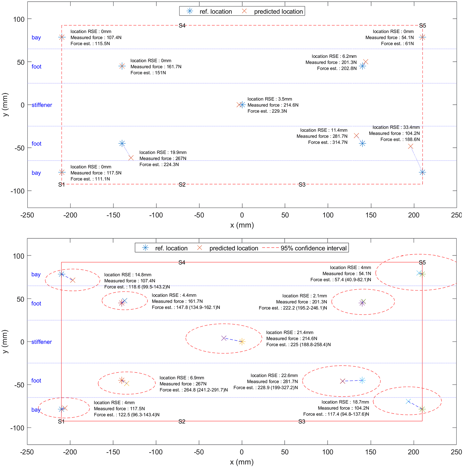
Example of location and maximum impact force estimation for impacts (case S1) on the stiffened panel using the benchmark deterministic method (top) and the proposed kriging stochastic method (bottom).

As mentioned in section ‘Introduction’, there are two main sources of uncertainty: measurement errors and algorithm inaccuracy.^7,14 The measurement errors are encoded in the reference database points, while the algorithm inaccuracy is represented in the multiple outputs given by feature combinations (section ‘Uncertainty quantification method for impact location and maximum force estimation’) which are merged with the proposed fusion methods. Because of this, the uncertainty range can be accurate and reliable, even though it is estimated only from the reference database points and not based on actual error measurements of the output. This also allows data-driven uncertainty quantification with a very low amount of reference database points (35) compared to other data-driven methods. An example is location uncertainty estimation with neural networks, as demonstrated by Sarego et al., ¹² which used 404 data points that were perturbed into 10,000 using the known uncertainty parameters (Monte Carlo approach). This highlights the suitability of the proposed data-driven method for uncertainty quantification by taking advantage of the information contained in their reference database without the need for expensive methods often used for this purpose (e.g. Monte Carlo simulations).^10,12

Conclusion

A novel data-driven stochastic kriging-based method for impact location and maximum force estimation was developed. Comparison with a deterministic benchmark method developed in prior studies^5,6,13 indicates that the proposed method gives more reliable estimates for experimental impacts under various simulated environmental and operational conditions by estimating the uncertainty. The developed method highlights the suitability of data-driven methods for uncertainty quantification by taking advantage of the relationship between data points in the reference database that is a mandatory component of these methods (and is often seen as a disadvantage). By quantifying the uncertainty, it gives more information for operators to reliably locate impacts and estimate the severity for making maintenance decisions.