Sage Journals: Discover world-class research

Abstract

This article presents a unique method of installing a special type of embedded ultrasonic transducers inside a 36-m-long section of an old bridge in Germany. A small-scale load test was carried out by a 16 ton truck to study the temperature and load influence on the bridge, as well as the performance of the embedded transducers. Ultrasonic coda wave interferometry technique, which has high sensitivity in detecting subtle changes in a heterogeneous medium, was used for the data evaluation and interpretation. The separation of two main influence factors (load effect and temperature variation) is studied, and future applications of wave velocity variation rate $Φ$ for structural health condition estimation are discussed. As a preliminary research stage, the installation method and the performance of the ultrasonic transducer are recognized. Load- and temperature-induced weak wave velocity variations are successfully detected with a high resolution of 10⁻⁴%. The feasibility of the whole system for long-term structural health monitoring is considered, and further research is planned.

Keywords

Structural health monitoring coda wave interferometry embedded transducer ultrasound bridge

Introduction

Bridges play an essential role in improving civil infrastructure and developing the economy. Environmental and mechanical factors or excessive use accelerate the deterioration of bridges. Over the past 20 years, more than 120 bridges have collapsed worldwide, causing economic losses and casualties. Many of them were due to the aging problem and untimely maintenance; most bridges still rely on temporary in-field non-destructive testing (NDT) methods to evaluate their condition and estimate damage. Various NDT techniques for concrete bridges are presented in Rehman et al.¹ Thus, real-time and long-term bridge condition assessment is becoming a focus of intense research. Structural health monitoring (SHM) is a promising technology that aims to monitor a structure during its whole service life, following all changes and events that occur in the structure, including geometric or elastic properties and defects, and so on. Therefore, a pre-warning can be given to avoid major losses before the condition of the bridge reaches a level that requires maintenance.

A great deal of literature on SHM has been published since the 1970s; however, there is still a gap between academic research and industrial applications.² A massive quantity of multiple types of SHM data on different structures has already been collected by researchers. One of the main difficulties we are facing is interpreting the collected data and separating different factors. As a consequence, the development of novel sensors and the upgrade of new algorithms are two crucial topics for SHM.

The most common long-term SHM techniques for bridge monitoring are mainly based on strain, displacement, and acceleration data collection. These data will be adopted to update the numerical model of the bridge in order to predict the structural behavior.³ Plenty of studies have presented a variety of sensors such as strain gauges (SG),^4–6 fiber optic sensors (FOS),^7–10 and accelerometers^11–13 to collect strain, displacement, and vibration acceleration data on real bridges. Though there are distinct advantages to using these sensors, they have a variety of drawbacks. SG is low-cost, efficient, and easy to install; however, due to its low durability, it can hardly meet the demands of long-term SHM. FOS has excellent endurance, and it also has a strong resistance to corrosion and electromagnetic interference. Distributed strain in a large area can be monitored by a single fiber line. Despite this, as fibers are fragile, particular layers and packaging material are required for protection. Extra care must be taken during the fiber installation. Moreover, depending on the acquisition frequency, the amount of data recorded by FOS is usually enormous, and the interrogators are normally costly. As most of these sensors are integrated on the surface of a structure, the influence of external environmental factors needs to be taken into account. Four representative applications of SHM on real bridges are listed as examples in Table 1.

Table 1.

Four bridge SHM examples.

Bridge	Influence factor	Sensor or technique	Physical quantity	Advantage	Drawbacks
Erqi Yangtze River Bridge¹³	Typhoon load	GPS, accelerometer, anemometer	Displacement, bridge natural frequency	Millimeter accuracy	Complex system, need data integration to improve accuracy
Binzhou Yellow River Highway Bridge¹⁴	Moving vehicle load	Fiber Bragg-grating (FBG)	Strain	High durability, high accuracy	Fragile, requires special packaging material
Ponte Moesa Bridge¹⁵	Damage	AE sensor	Elastic energy	Reliable to detect wires breaking	Noise disturbance, heavy data, deals with irreversible process but not steady state
Steinachtal Bridge¹⁶	Temperature	Geophone and CWI using passive noise	Wave propagation velocity change	High temporal resolution, low cost, high accuracy	Cementing on the surface, poor spatial resolution, difficult to localize origin

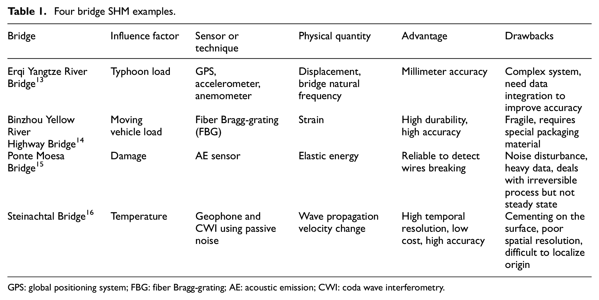
GPS: global positioning system; FBG: fiber Bragg-grating; AE: acoustic emission; CWI: coda wave interferometry.

As wave characteristics correlate to the physical and elastic properties of the material, performing active sonic methods on the surface of a structure has shown great efficiency for NDT. However, they have not yet been widely used for long-term SHM, especially inside a structure. According to existing studies, there are two different passive sonic methods: The proven solution is acoustic emission (AE),^17,18 which detects the energy release caused by a physical process such as the occurrence or development of damage. Early-stage damage can be detected and located¹⁹ by AE. However, the AE signals are normally weak; the noise in field conditions might greatly disturb the AE signals. Moreover, a huge amount of data is acquired during AE monitoring due to the high acquisition sampling rate, which increases the data processing cost. A brand new passive method was presented by Salvermoser et al. to monitor temperature-induced weak wave velocity variation in a bridge using the coda wave interferometry (CWI) technique.¹⁶ The passive wave was generated by the noise of vehicles passing the bridge’s expansion joints. Thus, this method relies on the traffic activity volume. Data were recorded by geophones cemented onto the inner surface of the box girder. The data analysis was concentrated in a low frequency range [2 Hz, 8 Hz], which caused poor spatial resolution, and the origin of velocity change could not be localized. The bridge was monitored for 2 months, and a health condition estimation using the temperature-induced velocity variation was discussed. These studies showed the possibility and potential of the CWI method for bridge SHM.

One solution to the shortcomings of passive CWI monitoring, expanding on the previous research, is to perform active monitoring in a higher frequency range inside the structure so that the scattering effect plays an important role. The interaction between the high-frequency signal and heterogeneities in the concrete ensures the sensitivity of the CWI technique. A special type of embedded US transducer, “SO807,” has been developed.²⁰ Studies have shown its solid performance and easy installation during the construction of concrete specimens^21–23 and a real bridge.²⁴ Nevertheless, it has not yet been implemented inside an existing old bridge.

The main influence factors on bridges are the temperature and traffic load. Both factors can cause a thermal and mechanical stress change.²⁵ When the stress applied to the concrete is below 40% of its compressive strength, the stress and strain follow a linear relationship (linear elastic behavior of concrete).²⁶ This relationship is given by the generalized Hooke’s Law as $σ_{ij} = E_{ijkl} ε_{kl}$ ,²⁵ where $σ_{ij}$ is the stress tensor, $ε_{kl}$ is the strain tensor, and $E_{ijkl}$ is the elastic constant. Hughes and Kelly²⁷ first derived the acousto-elastic parameter $Φ$ , which describes the ratio of the relative wave velocity variation to the change in stress based on Murnaghan’s theory.²⁸ Larose and Hall²⁹ related $Φ$ to the non-linear parameter $β$ , which depends on the elastic constant. $Φ$ can be expressed by $Φ = - β / E$ ,³⁰ where E is Young’s Modulus and is considered as a constant when the concrete is in the linear elastic phase. Planès and Larose then proposed an idea to evaluate the health condition of a structure by performing a small-scale load test in Planés and Larose.³¹ When the stress-induced $Φ_{S}$ exceeds a threshold, the structure needs maintenance. However, this threshold has not yet been clearly identified. Temperature plays different roles in different situations. During a long monitoring period, when the influence of the real-time traffic on a bridge is weak and, the temperature has a more significant impact, it can be used as a source to study the structural responses.^3,32 The temperature variation can cause a stress change. A linear relationship between the temperature variation and the corresponding strain change can be assumed and, consequently, can induce a linear stress change.²⁵ Sun and Zhu³³ confirmed that the temperature-induced $Φ_{T}$ is larger when the damage level in the tested specimen is higher. In the load test presented in this study, the load effect is the main research factor; thus, the temperature’s influence should be subtracted.

The aim of this study is to install a special type of embedded US transducer inside an old bridge using a unique installation method. As a first step, the bridge was monitored for 24 h and a small-scale load test was carried out to verify the feasibility of the installation method and to study the transducer’s performance. The CWI method was used for data analysis and separation of the temperature and load effect. Applications for long-term SHM purposes are considered. The experiment discussed here was carried out to evaluate the setup and the data-processing methods in advance of a large-scale load test which is due to take place in spring 2021.

Coda wave interferometry

“Coda” is an item first presented by Aki in the seismology domain, meaning the “tail” of a seismic wave recorded during an earthquake.^34,35 Later on, it was proposed for use in NDT purpose by Snieder and colleagues^36–38 using the later arrivals of a signal. When US measurement is performed in a high enough frequency range, waves enter a simple or multiple scattering regime and interact significantly with the heterogeneities.³¹ The wave propagation medium functions as an interferometer.³⁶ This is the origin of the CWI method. A coda wave is considered to be a superposition of all the scattered and reflected waves in the heterogeneous propagation medium; waves travel along a longer and more complicated path than the direct wave. Accordingly, the effect of a subtle change in the medium accumulates, leading to the high sensitivity of the CWI method. The wave propagation velocity is an essential parameter for analyzing and evaluating the condition of a structure as it is directly correlated with the propagation medium’s mechanical properties. Weak changes in the medium will cause a slight time perturbation. When the changes in the medium are relatively small, the time shift usually is undetectable by the first arrivals of a signal. Thus, the traditional mechanical property evaluation method, such as the ultra pulse velocity (UPV) test, is not applicable.

A recent method, “stretching,” was proposed in which weak time-scale perturbation is considered as dilation or expansion in time.³⁹ As the changes in the medium are amplified by the wave accumulation, time delay becomes wider and more recognizable in the later arrivals of the signal. This method requires two signals measured in two different states: the reference signal $u_{u} (t)$ recorded at the initial stage and the signal $u_{p} (t)$ recorded at a new stage after a small perturbation in the medium. Two useful features, the correlation coefficient (CC) and relative velocity change (dV/V), could be extracted by equation (1). $u_{p} (t)$ is stretched by a factor $α$ , which indicates a relative velocity increase or loss and then be expressed by $u_{u} (t (1 + α))$ . The $α_{best}$ , which maximizes the cross-correlation between $u_{u} (t)$ and $u_{p} (t)$ , is considered to be the dV/V

CC (α) = \frac{\int_{t - T}^{t + T} u_{u} (t^{'} (1 + α)) u_{p} (t^{'}) dt^{'}}{\sqrt{\int_{t - T}^{t + T} u_{u}^{2} (t^{'} (1 + α)) dt^{'} \int_{t - T}^{t + T} u_{p}^{2} (t^{'}) dt^{'}}}

(1)

The high sensitivity of the CWI method has been validated in detecting stress-induced velocity change,^22,40,41 temperature variation,^42–44 water saturation,^38,45 and early-stage damage.^22,23,46 The CWI method has also been applied for damage localization and imaging purposes.^21,47,48 The CWI method detects an overall change in the medium; velocity variations caused by different factors are not directly separated. According to existing studies, the two most common influence factors on wave propagation velocity change for most cases are stress and temperature, which are also the critical discussion factors in this study. Zhang proposed a thermal bias control technique to eliminate both the thermally induced velocity variation and the experimental bias from a load test in Zhang et al.⁴⁴ This method requires a second specimen with the same geometric size and concrete composition as the testing object as a reference. Measurements were performed on both specimens at the same time, except that no external stress was applied to the reference specimen. Thus, the $α$ (dV/V) measured by the reference specimen was mainly caused by the temperature and all additional experimental bias. According to his research, when the linear deformation $ε$ of the structure is relatively small, the overall $α$ can be expressed as equation (2)

α_{test} = α_{S} - ε_{S} + α_{T} - ε_{T} + α_{N}

(2)

where $α_{S}$ and $α_{T}$ represent the stress- and thermally induced $dV / V$ . $α_{N}$ is the additional experimental bias term. $ε_{S}$ and $ε_{T}$ are the linear deformation caused by stress and temperature. In this study, it is not possible to have another reference bridge. However, the weight of the truck used in this study is far less than the capacity of the bridge, and the temperature varied by less than 0.5 C. There was no rain nor snow. Thus, it can be assumed that $ε_{S}$ , $ε_{T}$ , and $α_{N}$ are negligible. The total dV/V can be expressed by equation (3)

α_{all} = α_{S} + α_{T}

(3)

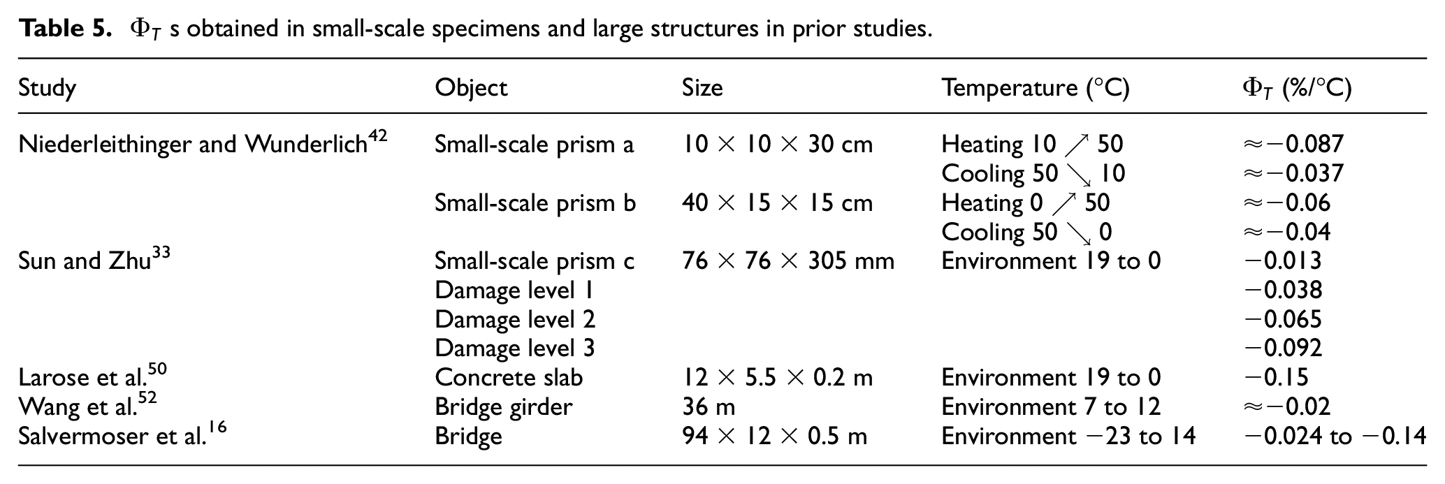
Various studies have shown the linear relationship between wave propagation velocity change and temperature variation.^42,43,49,50 Thus, the thermally induced velocity change during each truck position can be calculated by equation (4), where $T (p)$ is the temperature at the time when the truck was placed in different positions $p$ and $T_{start}$ is the temperature measured before the load test start

α_{T} (p) = Φ_{T} \times (T (p) - T_{start})

(4)

The $Φ_{T}$ can be calculated by equation (5), where $α_{end}$ represents the velocity change after the load test, after the truck had left. $T_{end}$ is the temperature measured after the load test. Alternatively, it could be estimated by the slope of the linear regression of the temperature-velocity curve if the bridge was to be monitored for a longer period

Φ_{T} = \frac{α_{end}}{T_{end} - T_{start}}

(5)

Experimental setup

The duraBASt bridge

“DuraBASt” is a demonstration, investigation, and reference area of the Germany Federal Highway Research Institute (BASt). It is located at the Cologne-East motorway junction (A3/A4) in Germany. There is a bridge on the site, which was built in 1973 but never put into operation. Different types of innovative sensors for humidity, corrosion, temperature and strain monitoring had already been installed under the road surface during the renewal of the bridge. The aim was the implementation of partial aspects of the “Intelligent Bridge.”

The tested section of the bridge for this study was a 36-m-long and 15-m-wide box girder bridge (Figure 1). Eight embedded ultrasonic transducers and one thermistor were installed inside the bridge’s lower section using a unique installation method. Detailed dimensions of the research object and locations of the sensors are presented in Figure 7.

Figure 1.

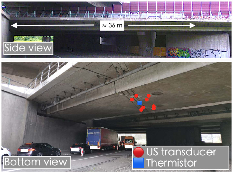
Side view and bottom view of duraBASt bridge.

Embedded US transducer and installation method

Conventional US transducers are normally glued onto the surface of the structure. The influence of external environmental factors has to be taken into account. Moreover, damages often appeared inside the structure and could not be detected by visual inspections of the structures. To focus more on the internal changes to the structure and provide an option for long-term SHM, a special type of embedded ultrasonic transducer, “SO807,” was developed. S0807 is a 7.5-cm-long hollow piezoelectric transducer (Figure 2). It could be operated as both transmitter and receiver. The primary frequency of SO807 is around 62 kHz, which is considered to be in the optimal frequency range for monitoring concrete using diffuse waves.⁵¹ The next step is to install the transducer on existing structures. Hence, a special method was developed in Niederleithinger et al.²⁰

Figure 2.

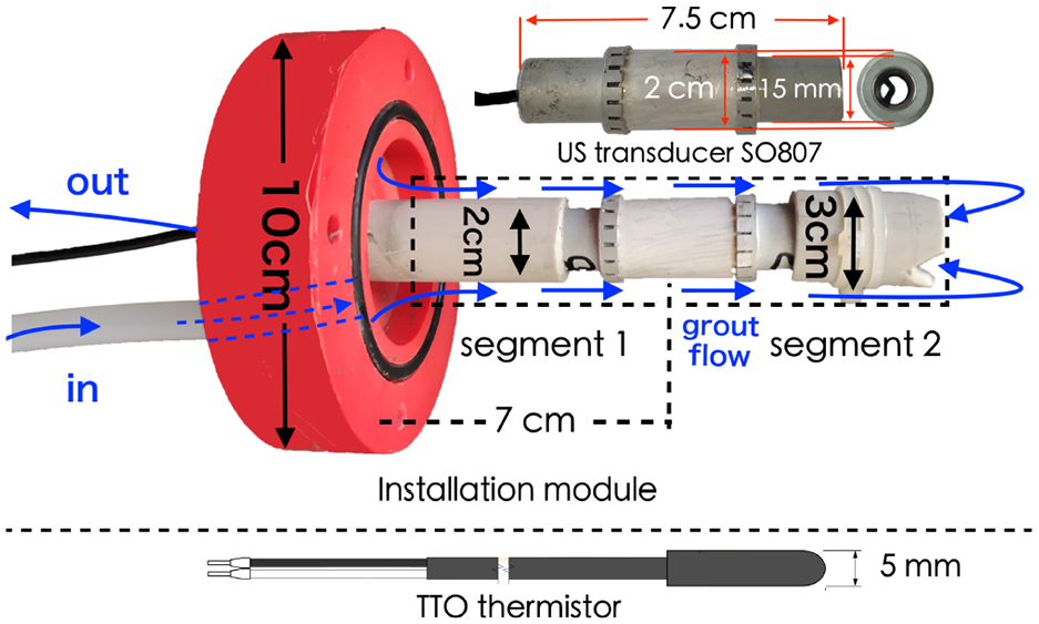
Transducer SO0807, sensor installation module, and thermistor TTO.

Figure 2 shows an “installation module” consisting of a plastic base with a rubber band to fix its position and ensure a strong sealing to the structure surface, as well as two PVC tube segments to control the depth. The segment at the end was wrapped by a self-locking cable, and a notch was cut to ensure the smooth circulation of the grout. As a first step, the installation method was tested on a small concrete cube in the laboratory by following these steps: (a) Drill a hole with a diameter of 3 cm and with the desired depth; (b) Insert the sensor installation module and fix with screws; (c) Seal the gap with glue; (d) Pump in the grout slowly using a Makita DCG180ZX cordless cartridge gun. A slightly expanding and fast hardening type of grout was used. Grout flow is shown by the blue arrows in Figure 2. The grout gradually filled the gap between the module and concrete. Once the hole was fully filled by the grout, the grout would come out through the hollow space of SO807 and the PVC tube. The inlet was then be blocked. Figure 3 shows the longitudinal section of the tested cube. This installation method provided sufficient coupling of the transducer to the concrete in the laboratory.

Figure 3.

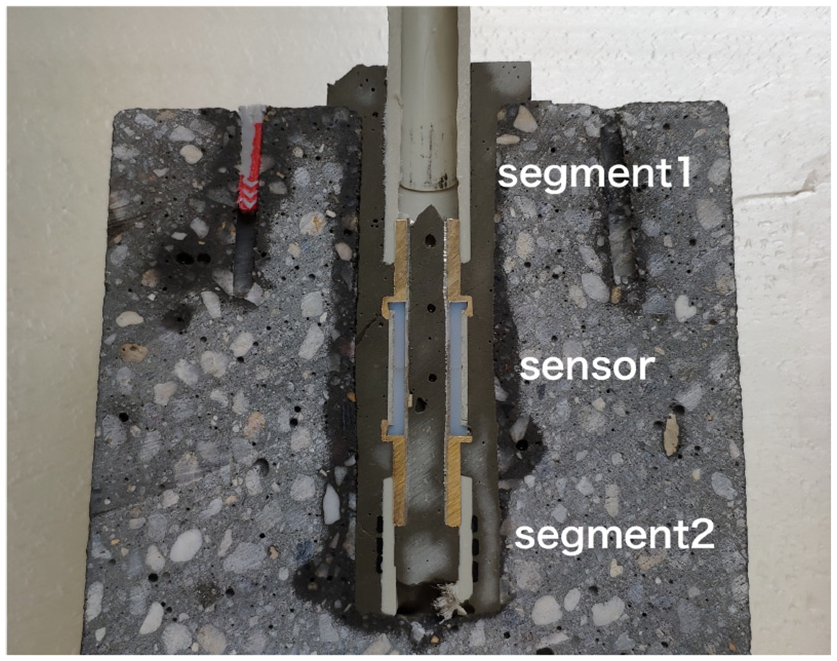
Longitudinal section of the tested specimen in laboratory.

It should be noted that the on-site installation was more complicated than that in the laboratory. The entire installation process followed Figure 4, and some processes are shown in Figure 5. Before drilling the hole in the desired position, an examination by ground-penetrating radar was carried out to avoid hitting the reinforcement. In unexpected situations, such as the presence of holes or a void (Figure 6, blue circle), the transducer position should be modified slightly. The positions of the transducers were designed to be at the four corners of a square with a side length of 1.06 m. However, they were all modified on-site. The actual positions of all the US transducers are shown in Figures 6 and 7. The eight transducers were divided into two groups for convenience: group A contains transducer Nos 1–4, which were located in the middle of line A, and group C contains transducers Nos.5-8, located on the line C. The distance between each pair of transducers (SxxEyy: transmitter No.xx, receiver No.yy) is presented in Table 2. A thermistor “TT0” from Tewa Temperature Sensors Ltd. was installed in the middle of the line between US transducer No.3 and No.7 using a similar installation method. All the cables were placed in PVC tubes for better protection.

Figure 4.

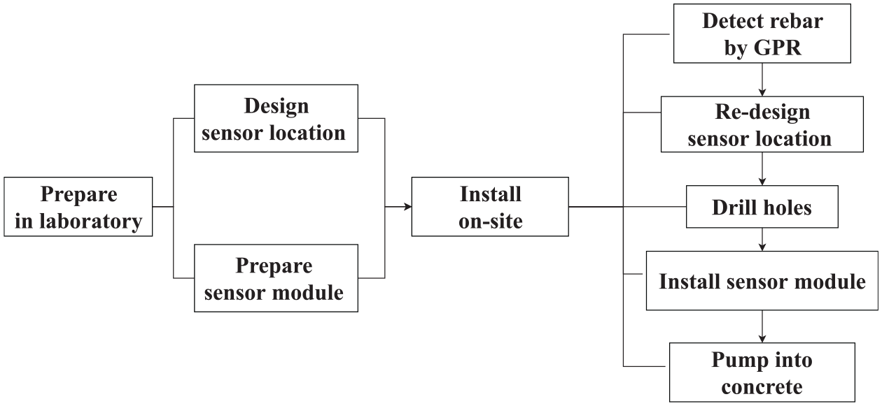
Diagram of the whole installation process.

Figure 5.

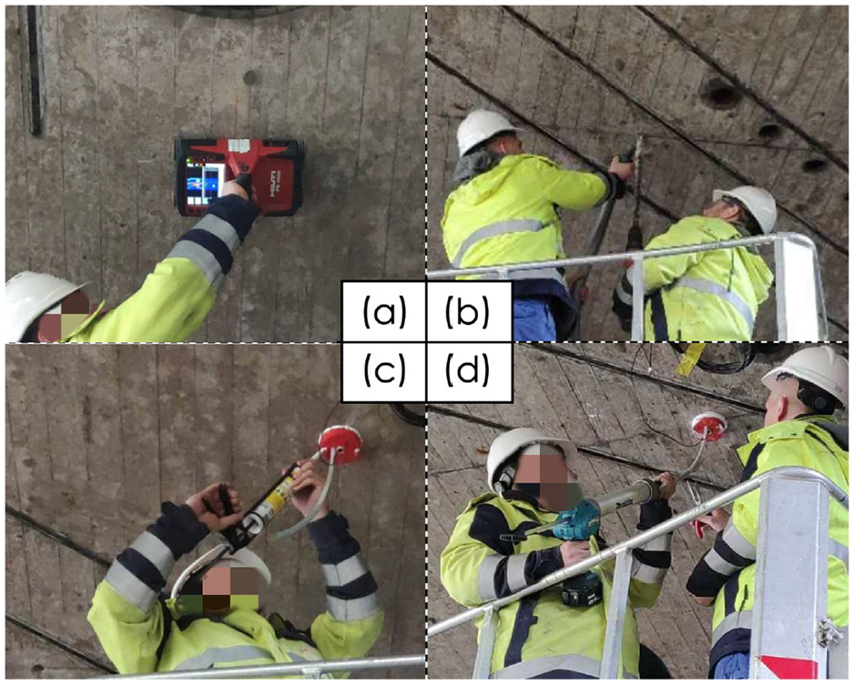
(a) Detect reinforcement by GPR, (b) drill hole, (c) seal the gap, and (d) pump in grout.

Figure 6.

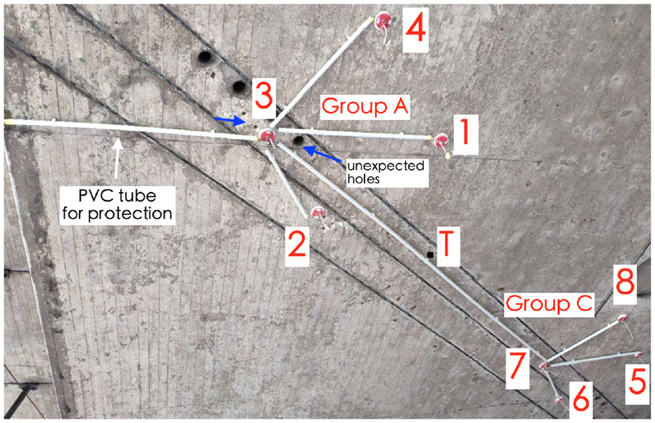
Actual position of all SO807 transducers and thermistor.

Figure 7.

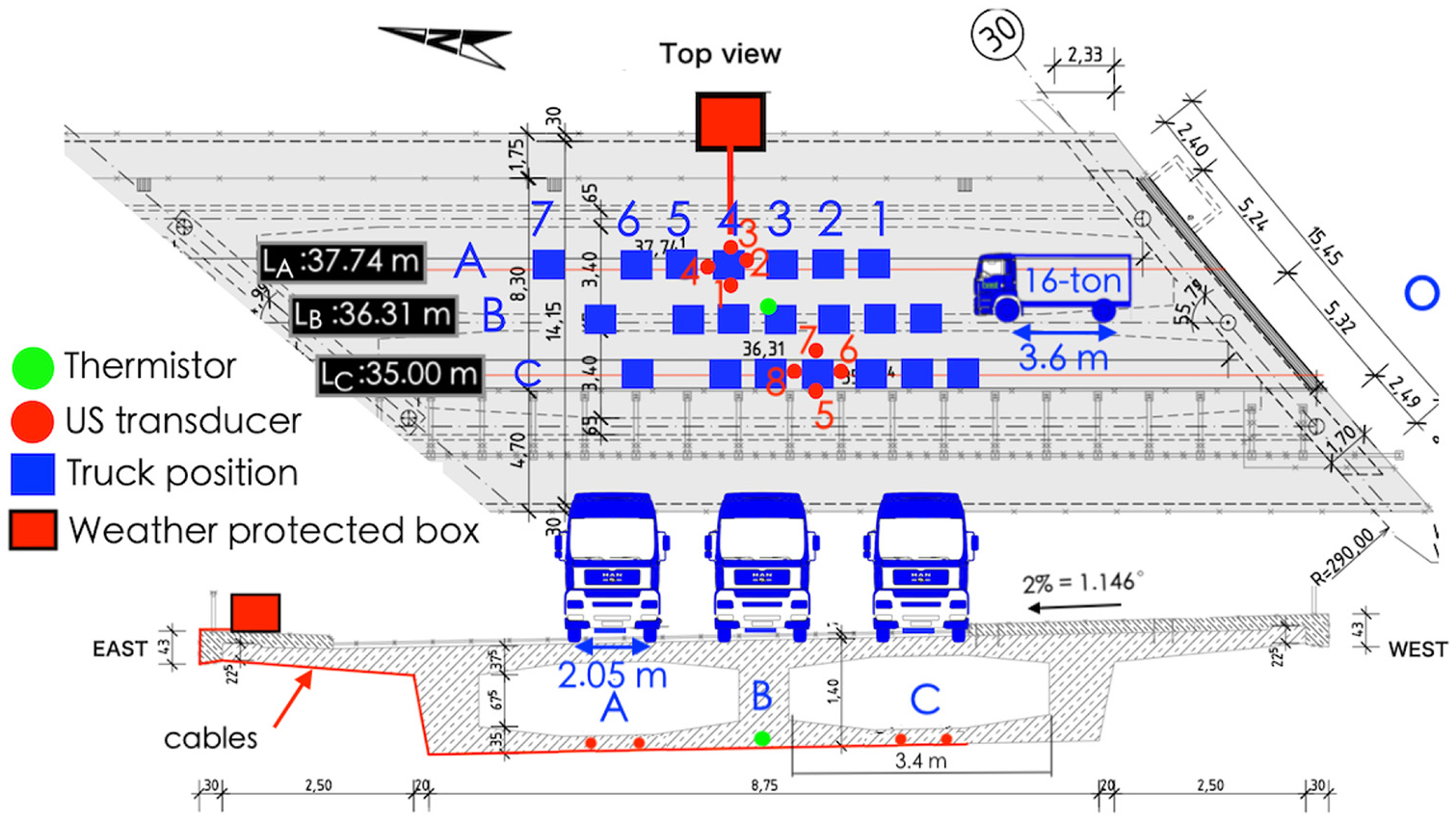
Sketch of the bridge, position of all sensors in top view, and all truck (load) positions along three lines.

Table 2.

Distance between transmitter–receiver (S-E) combinations in m.

S-E	S01E02	S01E03	S02E03	S02E04
Distance	1.14 m	1.37 m	0.86 m	1.58 m
S-E	S04E03	S07E05	S07E06	S07E08
Distance	1.09 m	1.55 m	1.07 m	1.12 m
S-E	S05E06	S08E06
Distance	1.24 m	1.77 m

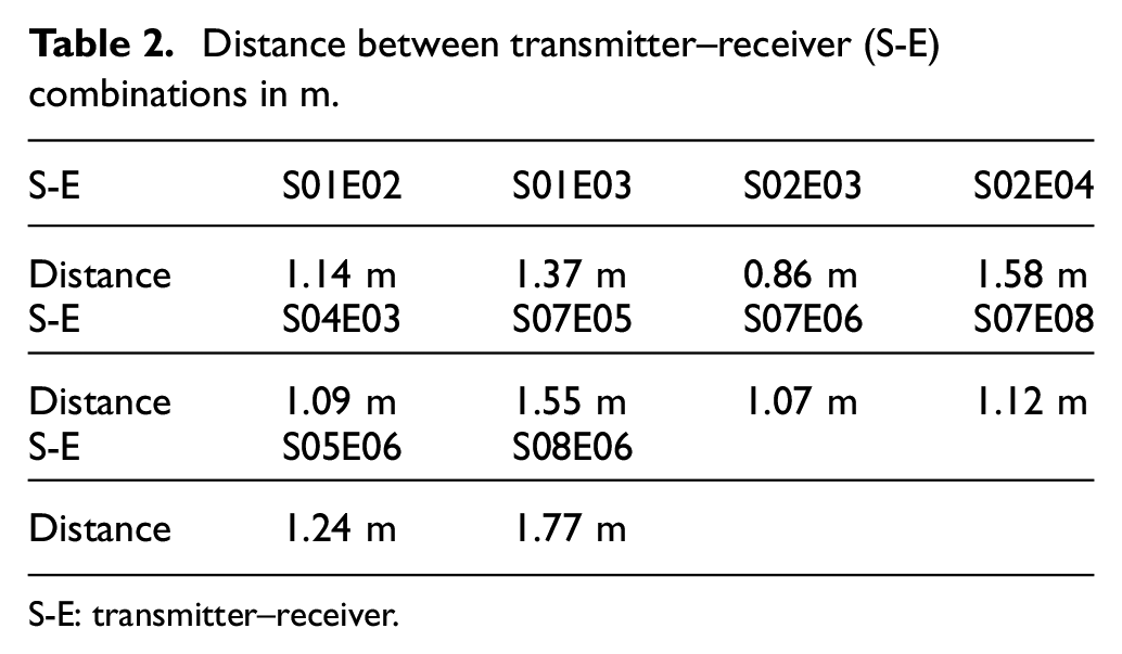
S-E: transmitter–receiver.

Experimental procedure

First, the bridge was monitored for 24 h on 6 October 2019, to study the temperature influence and to estimate the $Φ_{T}$ . The measurement interval was 5 min; thus, each transducer combination recorded 288 US signals. Four days later, a small-scale load test was performed. For the purpose of checking the whole experimental setup, the bridge was first monitored for 50 min from 08:18:28 to 09:04:32 on 10 October 2019, without any load. Then, a load test was performed by a 16 ton truck to study the influence of the load on the bridge as well as the performance of SO807 on order to evaluate the new installation method. The wheelbase of the truck was 3.6 m and the track was 2.05 m. The truck was placed in 21 positions (from A1 to C7) along three axes. Seven signals were recorded by each transducer combination at each truck location. The distance between every two positions from 1 to 6 was around 2 m and 4 m between positions 6 and 7. Axes A and C passed through the top of the transducers and are parallel to axis B, which was the midline of the bridge. The lengths of axes A, B, and C are around 37.74, 36.31, and 35 m. The layout of the truck positions and transducer locations is presented in Figure 7. The measurement periods on axes A, B, and C were from 09:12:45 to 10:08:11, from 10:11:25 to 11:07:29, and from 11:19:03 to 12:15:03, respectively. Measurement on each line lasted around 56 min.

Experimental results

US signals and noise

Environmental noise

All eight US transducers were performed as receivers to record the ambient environmental noise. The noises appeared randomly, but they all had similar amplitude and frequency components. The noises are most likely electromagnetic noise caused by the power line. Noises recorded by transducer No. 3 from group A and No. 5 from group C are, for example, presented in Figure 8 for instance. Their amplitudes varied in the range ±30 mV, which were relatively low, and the main noise frequencies were less than 40 kHz.

Figure 8.

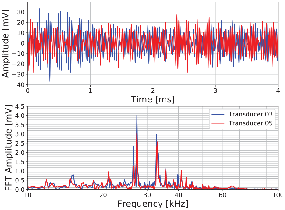
Environmental noise recorded by transducer Nos 3 and 5.

US signals

Figure 9 depicts a raw US data recorded by the data acquisition system used in this experiment. Due to the electromagnetic interference, a cross-talk was recorded when the excitation signal was triggered at 0.1 ms. A pre-processing procedure was required to remove the offset and crosstalk from the raw US data. Details of the procedure are presented in Niederleithinger et al.²¹ A pre-processed US signal recorded by transducer combination S02E03 and its corresponding amplitude spectrum (FFT) are illustrated in Figure 10 in black. Transducer SO807 is supposed to be most sensitive to 62 kHz, which is its central frequency. Thus, one of the main frequency distribution centers of the US signal is around 62 kHz. However, the other frequency components were distributed around 25 kHz. The authors assume that this is due to the stronger attenuation of higher frequency components and noise. To focus on the central frequency of SO807, the lower frequency components were filtered by a Butterworth band-pass filter (passband (40 kHz, 90 kHz), order 3) along with the noise. The filtered signal is shown in Figure 10 in red.

Figure 9.

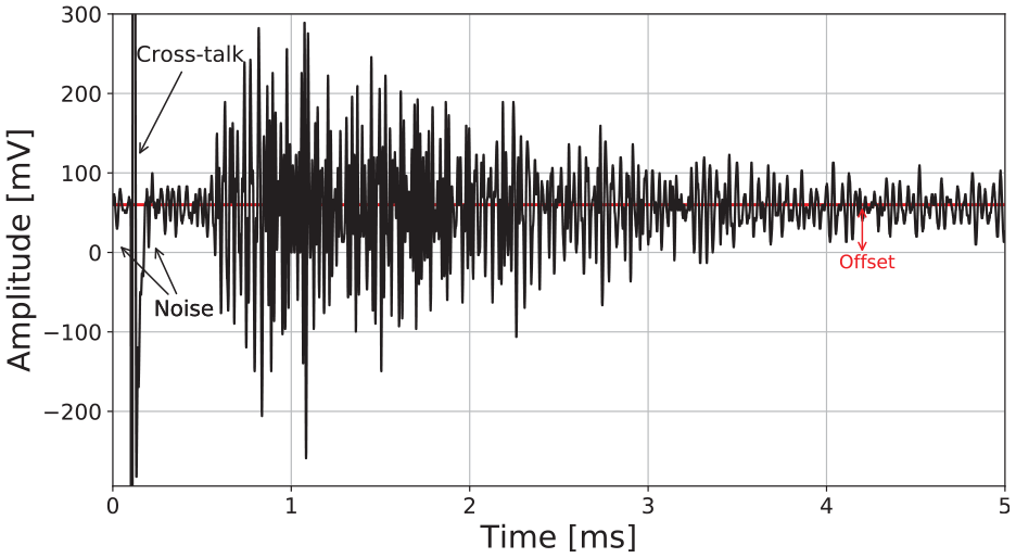
Raw US data recorded by the data acquisition system.

Figure 10.

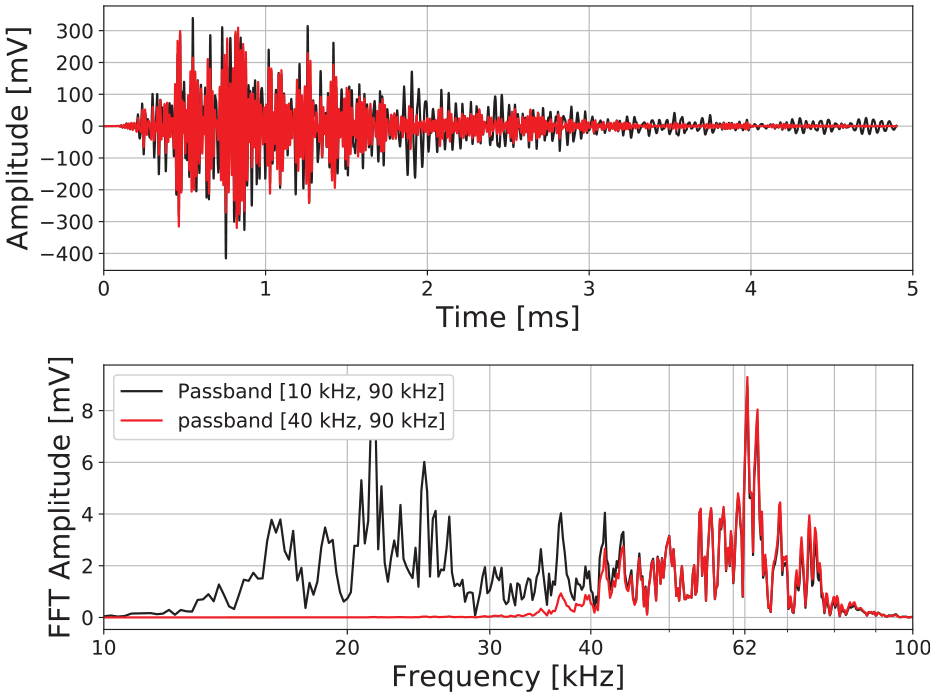
US data recorded by transducer combination S02E03 filtered by a band-pass filter with two passbands and their corresponding amplitude spectrum (FFT).

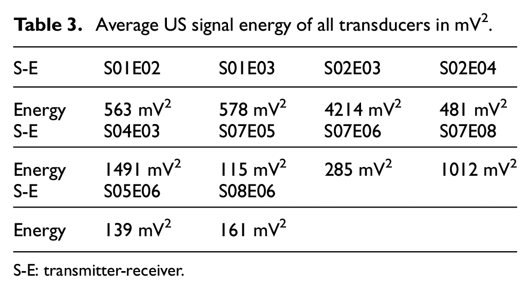
In general, when waves propagate through a different medium (i.e. from grout to concrete), they are often partially transmitted and partially reflected at the interface. That is to say, the wave can have some energy loss. The average energy of the filtered US signals recorded by all transducer combinations is presented in Table 3. By comparison, it is found that the signals recorded by transducers from group A had higher energy than those recorded by transducers from group C, with one exception: S07E08. There are various possible causes for this energy difference, for example, the coupling condition between transducer and concrete, varying reinforcements distribution, or existing voids or holes in the structure created for another purpose which appeared in-between or close to the direct path between two US transducers.

Table 3.

Average US signal energy of all transducers in mV².

S-E	S01E02	S01E03	S02E03	S02E04
Energy	563 mV²	578 mV²	4214 mV²	481 mV²
S-E	S04E03	S07E05	S07E06	S07E08
Energy	1491 mV²	115 mV²	285 mV²	1012 mV²
S-E	S05E06	S08E06
Energy	139 mV²	161 mV²

S-E: transmitter-receiver.

Coupling condition examination

As SO807 is a piezoelectric transducer, US signals are generated by the expansion and contraction of its piezoelectric ceramics part. When the transducer and concrete are coupled perfectly, the concrete absorbs the vibration of the piezoelectric ceramics part immediately. However, when the coupling condition is not ideal, the remaining vibration generates extra current and sends it back through the cable, which affects the cross-talk. Figure 11 depicts the crosstalk of two signals recorded under two coupling conditions. The imperfect coupling condition caused a damping of the crosstalk. Unfortunately, in this study, all eight SO807 transducers had imperfect coupling to the concrete. Nonetheless, their performance in this experiment still met the expectation that the US signals recorded by the SO807 transducers can be used to detect the temperature variation and different load positions. It is presumed that there are two types of imperfect coupling conditions. One is caused by the weathering of the grout, which creates a fine gap between the grout and the concrete. In this case, the US signal energy has a great loss. The other type is caused by the different damping ratio of the grout, which prevents the vibration energy of the ceramic part being absorbed in a short period.

Figure 11.

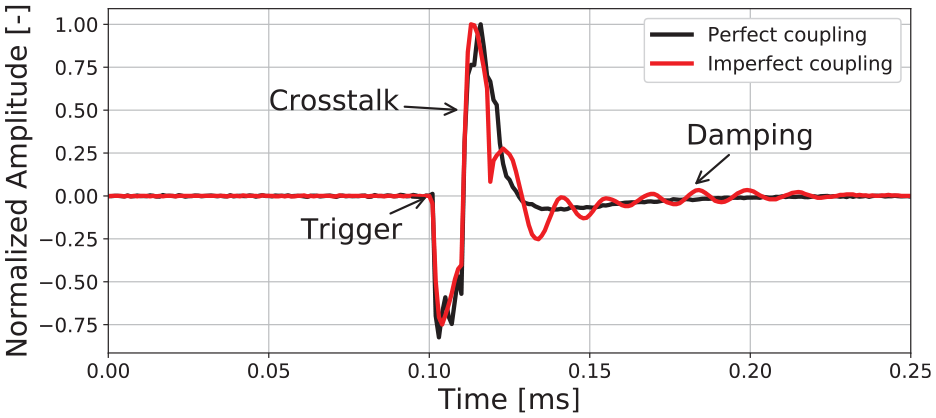
Influence of coupling condition on crosstalk at 1 ms.

Twenty-four-hour monitoring

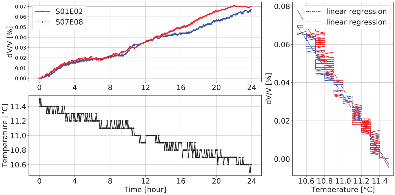
The bridge was monitored for 24 h. dV/Vs measured by transducer combination S01E02 and S07E08 are shown in Figure 12 as examples. During this period, the internal temperature of the bridge decreased 1°C from 11.5°C to 10.5°C. The dV/Vs increased almost linearly with the temperature. The slopes of the linear regression of the temperature-velocity curves are considered as the $Φ_{T}$ . The $Φ_{T}$ s of all the transducer combinations are listed in Table 4 as $Φ_{T} 1$ . Most of the $Φ_{T}$ s are around −0.1%/°C; the largest value was −0.157 %/°C, measured by transducer combination S02E03. Prior studies have obtained different $Φ_{T}$ s in different structures and under different temperature ranges. These $Φ_{T}$ s are summarized in Table 5. The $Φ_{T}$ s calculated in this study correspond well to the existing studies.

Figure 12.

dV/V, temperature variation, and the corresponding dV/V-temperature curve measured by transducer combination S01E02 and S07E08.

Table 4.

$Φ_{T}$ of all transducer combinations estimated by the slope of temperature-velocity curve $(Φ_{T} 1)$ measured during the 24-h monitoring and calculated according to the load test by equation (5) $(Φ_{T} 2)$ .

S-E	S01E02	S01E03	S02E03	S02E04	S04E03	S05E06	S07E05	S07E06	S07E08	S08E06
$Φ_{T} 1$ (%/°C)	−0.072	−0.104	−0.157	−0.125	−0.131	−0.037	−0.006	−0.100	−0.082	−0.025
$Φ_{T} 2$ (%/°C)	−0.032	−0.032	−0.015	−0.030	−0.040	−0.042	−0.035	−0.030	−0.020	−0.032

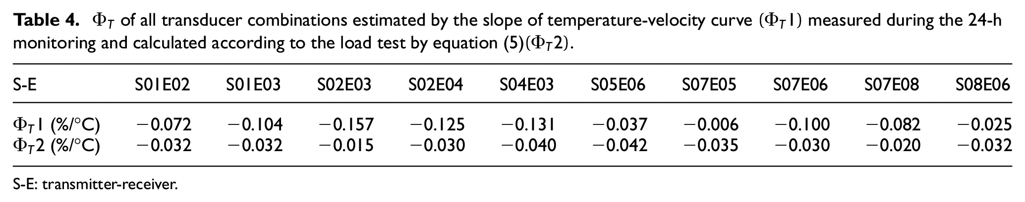
S-E: transmitter-receiver.

Table 5.

$Φ_{T}$ s obtained in small-scale specimens and large structures in prior studies.

Study	Object	Size	Temperature (°C)	$Φ_{T}$ (%/°C)
Niederleithinger and Wunderlich⁴²	Small-scale prism a	10 × 10 × 30 cm	Heating 10 ↗ 50	≈−0.087
			Cooling 50 ↘ 10	≈−0.037
	Small-scale prism b	40 × 15 × 15 cm	Heating 0 ↗ 50	≈−0.06
			Cooling 50 ↘ 0	≈−0.04
Sun and Zhu³³	Small-scale prism c	76 × 76 × 305 mm	Environment 19 to 0	−0.013
	Damage level 1			−0.038
	Damage level 2			−0.065
	Damage level 3			−0.092
Larose et al.⁵⁰	Concrete slab	12 × 5.5 × 0.2 m	Environment 19 to 0	−0.15
Wang et al.⁵²	Bridge girder	36 m	Environment 7 to 12	≈−0.02
Salvermoser et al.¹⁶	Bridge	94 × 12 × 0.5 m	Environment −23 to 14	−0.024 to −0.14

Fifty-minute non-load monitoring

The CC and dV/V measured by six transducer combinations located in both box girders, as well as the temperature variation, are shown in Figure 13 as an example. In comparison with the first reference signal, the maximum CC change was measured by transducer combination S07E05, which decreased to 0.9976. The maximum relative velocity change measured by these six transducer combinations was $1 \times 10^{- 2}$ %, and the minimum was $6 \times 10^{- 4}$ %. The CC of transducer combinations from group A varied less and more smoothly than that of transducer combinations from group C, for the reason that the CC measured the similarity of the signals, and the amplitudes of signals which had stronger energy were less affected by unexpected factors (i.e. noise). However, these signals were more sensitive to the relative velocity variation caused by the influence factors studied in this article (load and temperature). Temperature variation of less than 0.1°C was not detectable by the thermistor. Thus, the $Φ_{T}$ cannot be estimated by this monitoring. As the velocity increased linearly, the authors assume that the temperature decreased slightly.

Figure 13.

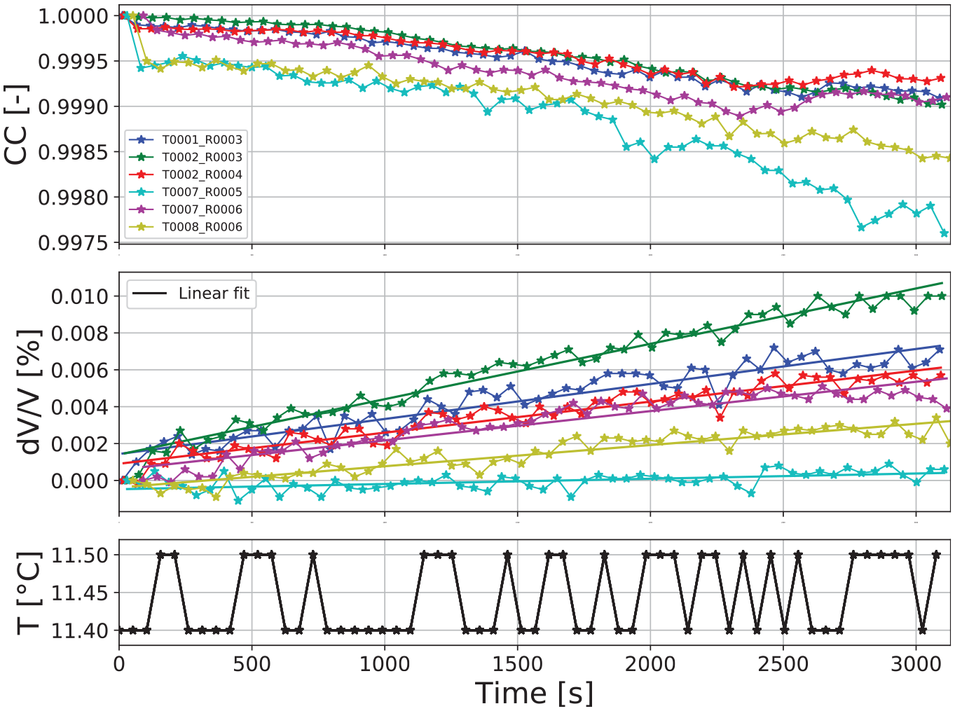
Correlation coefficient and relative velocity change of six transducer combinations during 50 min without load.

Load test

Temperature variation during the load test

The load test started at 09:12:45 and lasted for 3 h (around 1 h for each line). The temperature variation is shown in Figure 14 in black. The temperature increased by about 0.5°C during the whole load test. Due to the accuracy limit of the thermistor, the temperature fluctuated strongly by ±0.1°C. Assuming that the temperature remained the same during the measurement in each truck position, the average of all seven temperature measurements at each position was considered as the temperature (Figure 14 in red).

Figure 14.

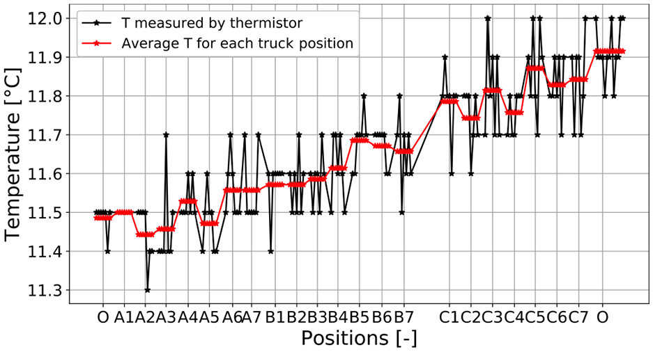
Temperature variation during the whole load test and average temperature of each truck position (O: without load).

Example of temperature-compensated dV/V

dV/V curves measured by transducer S02E03 along three lines are illustrated in Figure 15. When the truck left the bridge, dV/V returned to −0.009%, which was different from the initial state. For transducer combination S02E03, a temperature increase of 0.6°C led to a velocity loss of 0.009%; assuming the linear behavior, the $Φ_{T}$ of transducer combination S02E03 is then −0.015%/°C. $Φ_{T}$ s of all transducer combinations are listed in Table 4 as $Φ_{T} 2$ . Comparing to $Φ_{T} 1$ , the value of $Φ_{T} 2$ is much smaller and closer to the $Φ_{T}$ s found in another bridge in Wang et al.⁵² And $Φ_{T} 2$ was estimated by the signals measured during the load test; thus, the temperature effect in the dV/Vs was eliminated by $Φ_{T} 2$ . The curves with circle markers represent the relative velocity variation without temperature compensation, and curves with triangle markers describe the temperature compensated dV/V. dV/V successfully detected the 21 positions of the truck. However, the dV/V in each truck position did not remain stable but rather increased slightly, this being due to the residual influence of the previous truck position. The concrete takes time to recover to a stable state because of the creep effect. When the truck moved along line A, the dV/V decreased with a bigger range, as transducer combination S02E03 was located in the middle part of the line A. Likewise, the dV/V along line C decreased the least. As one can see, the temperature-induced dV/V compensation for lines A, B, and C increased gradually, which was following the temperature variation in Figure 14.

Figure 15.

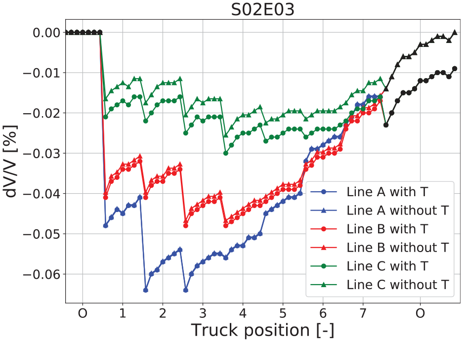
Relative velocity change and temperature compensated velocity change of transducer combination S02E03 in all seven positions of each lines.

CC and temperature-compensated dV/V of all transducer combinations

The CC and temperature-compensated dV/V measured by all transducer combinations are illustrated in Figures 16 and 17. The CC presented here is not temperature compensated as the CC is non-unique. The CC is not directly related to the elastic property of the material or the wave velocity change. Having said that, the CC can still provide some useful information as it measures the similarity between signals. Different truck positions can still be identified from some of the CC curves. It is notable that the CC of transducer combination S05E06 did not provide any useful information as it fluctuated too much. The average energy of the signals recorded by this transducer combination was 139 mV², which was weak, inferring that the coupling condition between transducer No. 5 and the concrete was poor. When transducer No. 5 was used as a transmitter, the wave energy had a more significant loss.

Figure 16.

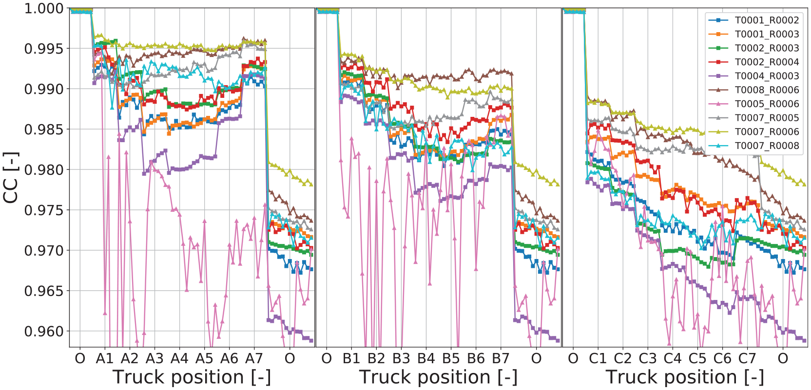
Correlation coefficient of all transducer combinations in all positions.

Figure 17.

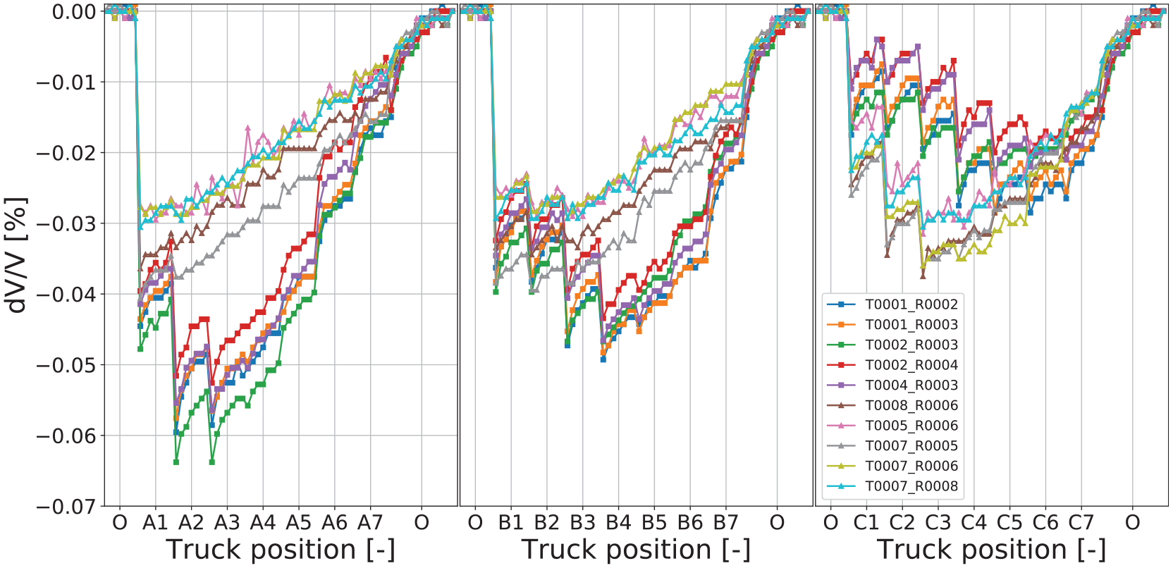
Temperature compensated relative velocity change of all transducer combinations in all positions.

The dV/Vs measured by transducer combinations from groups A and C are well separated. According to Figure 17 (left), when the truck moved along line A from position 1 to position 7, the dV/V of the transducer combinations from group A detected these different positions. The dV/V reached its lowest value when the truck moved to positions 3 and 4, which were located right above the transducers. The dV/V of the other transducer combinations from group C decreased to their minimum value when the truck was in position A1 and then started to increase approximately uniformly until it reached position A7. Because the truck was not located directly on line C, the influence of the load on the transducers from group C was lower. The effect of the load and of the residual influence from the previous truck position was superposed. Compared to when the truck was on line A, when the truck moved along line B, the overall dV/V of all group A transducer combinations increased and that of group C transducer combinations decreased, as the truck moved away from line A and got closer to line C. Figure 17 (right) shows the dV/V variation when the truck moved along line C. Most of the transducer combinations detected the different truck positions. Even transducer combination S05E06, which provided useless CC information, identified position C1, C2, and C3. When comparing the three dV/V graphs for the three lines, transducer combinations located along line A provided the clearest result for all 21 truck positions.

Discussion

There is a big difference between $Φ_{T} 1$ s and $Φ_{T} 2$ s, as shown in Table 4. The $Φ_{T} 1$ s were measured 4 days before the load test using the gradient of the temperature-velocity curves, while the $Φ_{T} 2$ s were simply calculated by the quotient of the dV/V difference and temperature difference before and after the load test, assuming their linear relation. When removing the temperature effect from the dV/Vs by $Φ_{T} 1$ , the dV/Vs detected by some transducer combinations exceeded 0, which is unusual, because, even if the creep effect still exists, the tensile stress should lead to a wave velocity decrease. Hence, we use $Φ_{T} 2$ to eliminate the temperature-induced dV/V. There are some possible causes for this error. As the accuracy of the thermistor was not high enough, the temperature values could have fluctuated too much. When the temperature changed in a range smaller than 0.6°C, which is at the boundary of resolution, the $T_{end}$ and $T_{start}$ might not present the actual temperature precisely. There was only one thermistor installed inside the middle part of the box girder, the temperature field inside the bridge is inhomogeneous; thus, there might have been a time shift between the outer and inner parts.⁵³ Despite this, this study still proposed an idea to remove the temperature effect, which works well.

During the 50-min non-load monitoring, the temperature variation was less than 0.1°C. The dV/V result validates the high sensitivity of the CWI method in detecting weak temperature-induced wave velocity variation with a resolution of 10⁻⁴%. The CC measured by higher energy US signals was less affected by the external factors. On the contrary, higher energy signals are more sensitive in detecting the weak velocity change and provide a more accurate dV/V curve.

Different truck positions were successfully detected by most of the transducer combinations to varying degrees. As the influence of the load on the bridge is greater and more direct than the temperature, unlike the non-load monitoring, the CC curves of all the transducer combinations which recoded higher energy signals decreased more and provided a more recognizable result for truck position identification. The influence of the temperature on the CC cannot be compensated. Along with the temperature increase, the CC values on lines A, B, and C decreased gradually.

The temperature-induced velocity variation was eliminated from the dV/V. The transducer combinations from group A had the best performance when the truck moved along all three lines, as the signals recorded by these transducer combinations have higher energy. They are more sensitive in detecting stress-induced velocity variation. When the truck moved along line A, due to the low energy of the signal, different truck positions could hardly be identified by the dV/V of the transduce combinations from group C. Nevertheless, when the truck moved along line C, dV/V measured by transducer combinations from group C decreased more than that measured by transducer combinations from group A. Besides, the length of line A was 37.74 m, which is 2.74 m longer than line C. Accordingly, the deflection caused by the truck on line A was bigger than on line C. This will also increase the velocity loss.

Conclusion and outlook

This study shows the feasibility of installing the SO807 embedded US transducers inside an old bridge using a unique installation method. The extremely high sensitivity of the CWI method in detecting load and temperature variation is validated. Although the coupling condition between the US transducers and concrete was not perfect, as a preliminary test stage, the performance of the US transducers was still satisfactory. In order to improve the coupling degree, different types of grout should be studied. As the damping appearing in the crosstalk was caused by the vibration of the transducer, an exponential curve-fitting model might be created to quantify the coupling condition. More experiments studying and re-verifying the temperature effect elimination method should be performed in the laboratory. A reference specimen should be prepared and precise internal temperature should be recorded with a higher degree of accuracy.

The data acquisition system used in this study can collect data continuously and support remote control. Thus, the whole system provides an option for long-term monitoring. The influence of the temperature on the bridge is not negligible, and it is one of the main influence factors on wave velocity variation. The thermistor has a lack of accuracy in the load test; however, it is accurate enough for long period monitoring. For long-term SHM, there is no need to eliminate the temperature influence. It is suggested that the temperature be used as a source. Bridge condition can be estimated by the temperature-included $Φ_{T}$ . Thus, it is planned to monitoring the bridge for a longer period (i.e. 6 months) to gain a better understanding of the $Φ_{T}$ .

The load at different truck positions was well detected. The next step is to quantify the load-induced velocity change and obtain the stress–velocity relationship, as Planès and Larose presented. In this case, the measurement will be finished in a short period of time, while the influence of the temperature will be negligible. Trucks of different weights will be placed at the same position (e.g. at the center of the bridge). Strain sensor should be installed to capture the internal stress change. The factor $Φ_{S}$ related to the health state of the structure can be observed from the slope of the linear regression of the dV/V-load curve.

If the coupling problem can be solved, then all the transducers will have similar performance. Thus, it is recommended to reduce the transducer numbers in practical applications. For example, only two US transducers installed in the middle of the bridge would be enough. Multiple US transducers can be also installed along the length of the bridge at intervals of 2 m to cover a larger area. The authors conclude that there are two ways to evaluate the bridge condition, the first one being temperature-induced $Φ_{T}$ for the purpose of long-term SHM. Data will be collected continuously with a larger measuring interval (i.e. 0.5 h) and be processed directly. Monthly or weekly $Φ_{T}$ can be obtained to monitor the bridge. The second method is based on the temporary in-field NDT measurement using trucks with different loads to obtain the stress-induced $Φ_{S}$ . This examination could be done twice a year. As we are still in the early stage of the research, more studies and experiments have to be done to have a better understanding of $Φ_{S}$ and $Φ_{T}$ . The threshold of $Φ_{S}$ and $Φ_{T}$ should be defined to find the concrete condition transition between healthy and damaged. An SHM standard using $Φ_{S}$ and $Φ_{T}$ could then be set in the future.

In conclusion, the installation method and the CWI technique for SHM have great potential and have a lot of room for expansion.

Footnotes

Acknowledgements

This research object was supported by BASt (German Federal Highway Research Institute). Thank you Mr. Peter Haardt and Mrs. Iris Hindersmann from BASt for providing me with convenience. Thank you Mr. Marco Lange and Mr. Heiko Stolpe from BAM for helping me install the transducers. Thank you Daniel Fontoura Barroso for developing the thermistor data acquisition module.

Declaration of conflicting interests

The author(s) declared no potential conflicts of interest with respect to the research, authorship, and/or publication of this article.

Funding

The author(s) disclosed receipt of the following financial support for the research, authorship, and/or publication of this article: This research work was performed within the European project INFRASTAR, Innovation and Networking for Fatigue and Reliability Analysis of Structures-Training for Assessment of Risk (infrastar.eu), which has received funding from the European Union’s Horizon 2020 research and innovation program under the Marie Skłodowska-Curie Grant No. 676139.

ORCID iD

Xin Wang

References

Rehman

SKU

Ibrahim

Memon

, et al. Nondestructive test methods for concrete bridges: a review. Constr Build Mater 2016; 107: 58–86.

Cawley

Structural health monitoring: closing the gap between research and industrial deployment. Struct Health Monit 2018; 17(5): 1225–1244.

Kromanis

Kripakaran

SHM of bridges: characterising thermal response and detecting anomaly events using a temperature-based measurement interpretation approach. J Civ Struct Health Monit 2016; 6(2): 237–254.

Brownjohn

Moyo

Omenzetter

, et al. Lessons from monitoring the performance of highway bridges. Struct Control Health Monit 2005; 12(3–4): 227–244.

Cardini

DeWolf

JT.

Long-term structural health monitoring of a multi-girder steel composite bridge using strain data. Struct Health Monit 2009; 8(1): 47–58.

Sanayei

Phelps

Sipple

, et al. Instrumentation, nondestructive testing, and finite-element model updating for bridge evaluation using strain measurements. J Bridge Eng 2012; 17(1): 130–138.

Casas

Cruz

PJ.

Fiber optic sensors for bridge monitoring. J Bridge Eng 2003; 8(6): 362–373.

Bastianini

Matta

Rizzo

, et al. Overview of recent bridge monitoring applications using distributed Brillouin fiber optic sensors. J Nondestruct Test 2007; 12(9): 269–276.

Minardo

Bernini

Amato

, et al. Bridge monitoring using Brillouin fiber-optic sensors. IEEE Sens J 2011; 12(1): 145–150.

10.

Sigurdardottir

Glisic

On-site validation of fiber-optic methods for structural health monitoring: Streicker bridge. J Civ Struct Health Monit 2015; 5(4): 529–549.

11.

Jang

Cho

, et al. Structural health monitoring of a cable-stayed bridge using smart sensor technology: deployment and evaluation. Smart Struct Syst 2010; 6(5–6): 439–459.

12.

Bao

Beck

Compressive sampling for accelerometer signals in structural health monitoring. Struct Health Monit 2011; 10(3): 235–246.

13.

Han

Wang

Meng

, et al. Analysis of the dynamic response of a long span bridge using GPS/accelerometer/anemometer under typhoon loading. Eng Struct 2016; 122: 238–250.

14.

Zhao

, et al. Structural health monitoring system for the Shandong Binzhou Yellow River highway bridge. Comput-Aided Civ Infrastruct Eng 2006; 21(4): 306–317.

15.

Vogel

Schechinger

Fricker

Acoustic emission analysis as a monitoring method for prestressed concrete structures. Zürich: Institute of Structural Engineering, ETH Zürich, 2006.

16.

Salvermoser

Hadziioannou

Stähler

SC.

Structural monitoring of a highway bridge using passive noise recordings from street traffic. J Acoust Soc Am 2015; 138(6): 3864–3872.

17.

Lovejoy

SC.

Acoustic emission testing of beams to simulate SHM of vintage reinforced concrete deck girder highway bridges. Struct Health Monit 2008; 7(4): 329–346.

18.

Grosse

McLaskey

Bachmaier

, et al. A hybrid wireless sensor network for acoustic emission testing in SHM. In: Proceedings of the sensors and smart structures technologies for civil, mechanical, and aerospace systems, 2008, vol. 6932, p. 693238. Bellingham, WA: The International Society for Optics and Photonics, http://glaser.berkeley.edu/glaserdrupal/pdf/SPIE%2008%20mclaskey-glaser-grosse-etc.pdf

19.

Grosse

Ohtsu

Acoustic emission testing. Berlin: Springer Science & Business Media, 2008.

20.

Niederleithinger

Wolf

Mielentz

, et al. Embedded ultrasonic transducers for active and passive concrete monitoring. Sensors 2015; 15(5): 9756–9772.

21.

Niederleithinger

Wang

Herbrand

, et al. Processing ultrasonic data by coda wave interferometry to monitor load tests of concrete beams. Sensors 2018; 18(6): 1971.

22.

Bassil

Wang

Chapeleau

, et al. Distributed fiber optics sensing and coda wave interferometry techniques for damage monitoring in concrete structures. Sensors 2019; 19(2): 356.

23.

Wang

Chakraborty

Bassil

, et al. Detection of multiple cracks in four-point bending tests using the coda wave interferometry method. Sensors 2020; 20(7): 1986.

24.

Wang

Chakraborty

Klikowicz

, et al. Monitoring a concrete bridge girder with the coda wave interferometry method. In: Proceedings of the 5th international conference on smart monitoring, assessment and rehabilitation of civil structures, Potsdam, 2019, pp. 27–29, https://infrastar.eu/fileadmin/contributeurs/Infrastar/Outreach_Dissemination/Publications/2019_08_SMAR_Xin.pdf

25.

Gould

PL.

Introduction to linear elasticity, vol. 346. Berlin: Springer, 2013.

26.

Kmiecik

Kamiński

Modelling of reinforced concrete structures and composite structures with concrete strength degradation taken into consideration. Archiv Civ Mech Eng 2011; 11(3): 623–636.

27.

Hughes

Kelly

Second-order elastic deformation of solids. Phys Rev 1953; 92(5): 1145.

28.

Murnaghan

FD.

Finite deformation of an elastic solid. New York: Wiley, 1951.

29.

Larose

Hall

Monitoring stress related velocity variation in concrete with a 2x10(–5) relative resolution using diffuse ultrasound. J Acoust Soc Am 2009; 125(4): 1853–1856.

30.

Schurr

Kim

Sabra

, et al. Monitoring damage in concrete using diffuse ultrasonic coda wave interferometry. AIP Conf Proc 2011; 1335: 1283–1290.

31.

Planés

Larose

A review of ultrasonic coda wave interferometry in concrete. Cem Concrete Res 2013; 53: 248–255.

32.

Xia

Cheng

Zhang

, et al. In-service condition assessment of a long-span suspension bridge using temperature-induced strain data. J Bridge Eng 2017; 22(3): 04016124.

33.

Sun

Zhu

Thermal modulation of nonlinear ultrasonic wave for concrete damage evaluation. J Acoust Soc Am 2019; 145(5): EL405–EL409.

34.

Aki

Analysis of the seismic coda of local earthquakes as scattered waves. J Geophys Res 1969; 74(2): 615–631.

35.

Aki

Chouet

Origin of coda waves: source, attenuation, and scattering effects. J Geophys Res 1975; 80(23): 3322–3342.

36.

Snieder

Grêt

Douma

, et al. Coda wave interferometry for estimating nonlinear behavior in seismic velocity. Science 2002; 295(5563): 2253–2255.

37.

Snieder

Coda wave interferometry and the equilibration of energy in elastic media. Phys Rev E 2002; 66(4): 046615.

38.

Grêt

Snieder

Scales

Time-lapse monitoring of rock properties with coda wave interferometry. J Geophys Res Solid Earth 2006; 111(B3): B03305.

39.

Sens-Schönfelder

Wegler

Passive image interferometry and seasonal variations of seismic velocities at Merapi Volcano, Indonesia. Geophys Res Lett 2006; 33(21): L21302.

40.

Stähler

Sens-Schönfelder

Niederleithinger

Monitoring stress changes in a concrete bridge with coda wave interferometry. J Acoust Soc Am 2011; 129(4): 1945–1952.

41.

Wang

Niederleithinger

Coda wave interferometry used to detect loads and cracks in a concrete structure under field conditions. In: Proceedings of the 9th European workshop on structural health monitoring series, Manchester, 10–13 July 2018, pp. 10–13. Berlin: Federal Institute for Materials Research and Testing.

42.

Niederleithinger

Wunderlich

Influence of small temperature variations on the ultrasonic velocity in concrete. AIP Conf Proc 2013; 1511: 390–397.

43.

Livings

Dayal

Barnard

Coda wave interferometry for the measurement of thermally induced ultrasonic velocity variations in CFRP laminates. AIP Conf Proc 2016; 1706: 120003.

44.

Zhang

Abraham

Tournat

, et al. Validation of a thermal bias control technique for coda wave interferometry (CWI). Ultrasonics 2013; 53(3): 658–664.

45.

Legland

Abraham

Villain

, et al. Suivi du gradient de teneur en eau dans les bétons par modulation non linéaire de la coda ultrasonore. In: Proceedings of the CFA, 2016, https://www.researchgate.net/publication/301301719_Suivi_du_gradient_de_teneur_en_eau_dans_les_betons_par_modulation_non_lineaire_de_la_coda_ultrasonore

46.

Schurr

Kim

Sabra

, et al. Damage detection in concrete using coda wave interferometry. NDT&E Int 2011; 44(8): 728–735.

47.

Zhang

Planes

Larose

, et al. Diffuse ultrasound monitoring of stress and damage development on a 15-ton concrete beam. J Acoust Soc Am 2016; 139(4): 1691–1701.

48.

Larose

Obermann

Digulescu

, et al. Locating and characterizing a crack in concrete with diffuse ultrasound: a four-point bending test. J Acoust Soc Am 2015; 138(1): 232–241.

49.

Güneyli

Karahan

Güneyli

Water content and temperature effect on ultrasonic pulse velocity of concrete. Russ J Nondestruct Test 2017; 53(2): 159–166.

50.

Larose

de Rosny

Margerin

, et al. Observation of multiple scattering of kHz vibrations in a concrete structure and application to monitoring weak changes. Phys Rev E 2006; 73(1): 016609.

51.

Fröjd

Ulriksen

Frequency selection for coda wave interferometry in concrete structures. Ultrasonics 2017; 80: 1–8.

52.

Wang

Chakraborty

Niederleithinger

Noise reduction for improvement of ultrasonic monitoring using coda wave interferometry on a real bridge. J Nondestruct Eval 2021; 40: 14.

53.

Epple

Barroso

Niederleithinger

. Towards monitoring of concrete structures with embedded ultrasound sensors and coda waves—first results of DFG for CoDA. In: Proceedings of the European workshop on structural health monitoring (EWSHM 2020), Palermo, 6–9 July 2020.

The installation of embedded ultrasonic transducers inside a bridge to monitor temperature and load influence using coda wave interferometry technique

Abstract

Keywords

Introduction

Coda wave interferometry

Experimental setup

The duraBASt bridge

Embedded US transducer and installation method

Experimental procedure

Experimental results

US signals and noise

Environmental noise

US signals

Coupling condition examination

Twenty-four-hour monitoring

Fifty-minute non-load monitoring

Load test

Temperature variation during the load test

Example of temperature-compensated dV/V

CC and temperature-compensated dV/V of all transducer combinations

Discussion

Conclusion and outlook

Footnotes

Acknowledgements

Declaration of conflicting interests

Funding

ORCID iD

References