Sage Journals: Discover world-class research

Abstract

This study is devoted to the use of acoustic emission technique for a comprehensive damage assessment, that is, damage detection, localization, and classification, of an aeronautical metal-to-composite bonded panel. The structure comprised a titanium panel adhesively bonded to carbon fiber–reinforced plastic omega stringers. The panel contained a small initial artificial debonding between the titanium panel and one of the carbon fiber–reinforced plastic stringers. The panel was subjected to a cyclic increasing in-plane compression load, including loading, unloading, and then reloading to a higher load level, until the final fracture. The generated acoustic emission signals were captured by the acoustic emission sensors, and digital image correlation was also used to obtain the strain field on the surface of the panel during the test. The results showed that acoustic emission can accurately detect the damage onset, localize it, and also trace its evolution. The acoustic emission results not only were consistent with the digital image correlation results, but also managed to detect the damage initiation earlier than digital image correlation. Finally, the acoustic emission signals were clustered using particle swarm optimization method to identify the different damage mechanisms. The results of this study demonstrate the capability of acoustic emission for the comprehensive damage characterization of aeronautical bi-material adhesively bonded structures.

Keywords

Bi-material adhesively bonded joint structural health monitoring debonding acoustic emission digital image correlation

Introduction

With the increased awareness toward environmentally sustainable industries, especially in aviation and automotive industries, the need for fuel-efficient vehicles, and consequently less carbon dioxide (CO₂) emissions, becomes inevitable. There are various approaches to achieve this objective; one of which, particularly in aerospace industry, is improving the structure’s aerodynamics and reducing the drag. This can be achieved by creating a laminar boundary layer flow rather than the conventional turbulent boundary layer flow. Srinivasan and Bertram¹ reported that approximately 50% of the total aircraft drag during cruise is due to friction drag, which is almost 10 times lower in the case of laminar flow as opposed to turbulent flow.

Hybrid laminar flow control (HLFC) is one of the techniques developed to delay the transition from a laminar to turbulent boundary layer flow. HLFC can be obtained by integrating suction areas in the leading edges of the wing, for instance.² A promising structural solution is the combination of a micro-drilled outer titanium surface adhesively bonded with an inner composite structure.¹ However, in the case of shear loading or axial compression or a combination of both, the stiffened titanium-to-composite panels are susceptible to buckling failure. Thus, the proper understanding and investigation of the buckling and post-buckling behavior of such structures are inevitable. In the open literature, the response of open cross-sectional stiffeners, such as I-, C-, and T-stringers, was extensively discussed,^3–13 while less attention^1,14–16 was drawn to closed cross-sections such as omega shape stringers, although they exhibit higher bending and torsional stiffness¹⁶ when connected to the skin.

Regardless of the stringer’s choice and as can be anticipated, different damage mechanisms may occur in the stiffened panel, such as the skin failure, the stringer failure, and the debonding of the stringer–skin interface. The debonding is usually treated as the most critical damage type. This damage is usually invisible or barely visible, but it can considerably affect the integrity and stability of the structure, and finally leads to a catastrophic failure.¹⁷ Therefore, in situ monitoring of the damage is essential to provide a reliable and safe aeronautical stiffened structure. Some non-destructive testing (NDT) techniques, such as guided wave and ultrasonic scan (UT), have been already used for damage detection in the stiffened panels.^17–22 However, these techniques are time-consuming and can only be carried out offline. Structural health monitoring (SHM) proposes continuous monitoring of the integrity of the structure by employing different techniques that have the capability of in situ monitoring, such as acoustic emission (AE) and fiber optic sensor.^23–29 Dávila and Bisagni³⁰ performed a multi-instrumented compression fatigue test on the single-stringer-stiffened carbon fiber–reinforced plastic (CFRP) panels. They used UT, passive thermography, high-speed camera, and digital image correlation (DIC) to detect the propagation of the artificial debonding and to track the sequence of damage mechanisms up to the final fracture. The post-buckling deformation was captured by DIC. The passive thermography detected the onset of the artificial debonding growth and UT precisely sized it. The high-speed camera highlighted that the instantaneous final fracture occurred due to the stringer–skin debonding followed by the stringer crippling. The utilized techniques have some limitations that restrict employing them for the monitoring of a real structure. For example, as aforementioned, UT could not be used as an online monitoring technique, and the inspection area of thermography and DIC techniques was not wide enough to monitor the real large structures. Vanniamparambil et al.³¹ used AE and ultrasonic guided wave to detect the debonding onset and also to track its evolution at the spar–skin interface of the CFRP-stiffened panel subjected to the fatigue loading. The results showed that the onset of the debonding was characterized by low-frequency and high-duration AE signals. Besides, the damage index, defined based on the recorded guided waves, was sensitive to the enlargement of the debonding area. Kolanu et al.³² investigated the failure of a CFRP-stiffened panel subjected to the compression loading using AE, DIC, infrared thermography, and strain gauges. DIC captured the strain distributions during the buckling and post-buckling, while strain gauges could precisely detect the onset of buckling. However, because of the sudden final failure, they could not detect the initiation and propagation of the catastrophic damage properly. While the AE effectively detected and classified different damage mechanisms in the panel, the thermography images were used to verify the AE results and also to localize the delamination region in the panel.

Although AE has been proven, in the open literature, as a well-established and effective tool in SHM, especially for composite structures, there is a significant gap of knowledge when it comes to three main challenges. These challenges can be summarized as follows: (1) the use of AE in SHM of bi-material structures, (2) the comprehensive damage assessment fulfilling the four levels of SHM, that is, damage initiation detection, damage classification, damage severity assessment, and damage localization, and (3) the reliability of the damage classification. Thus, in this study, a comprehensive AE-based damage assessment was performed that fulfills all the four levels of SHM for a bi-material stiffened panel resembling an aeronautical structure as a benchmark. Moreover, a robust evolutionary optimization technique was employed for the AE damage clustering that significantly increases the reliability of the SHM system by overcoming the disabilities of the commonly used clustering techniques in the literature, that is, K-means, fuzzy-c-means, and self-organizing map.^23,33

Materials and manufacturing

Two panels were fabricated of titanium grade 2 of 0.8 mm thickness stiffened by omega CFRP stringers. The layup of the CFRP stringers was [0/45/45/0] for the inner laminate and [90/−45/−45/90] for the outer laminate. They were made from a five-harness weave fabric Hexforce G0926 from Hexcel with a 6K HS carbon fiber and an areal weight of 370 gsm and RTM6 resin from Hexcel. An adhesive film was used between the quasi-isotropic composite laminate and the titanium. The adhesive and RTM6 resin were cured in one cycle together to bond the titanium to the omega stringers. The foam core was made of Rohacell Hero 71-10. To create an artificial debonding, an Upilex-25S foil of 0.025 mm thickness was placed in between one of the stringers and the titanium sheet. No adhesive was used at the location of the Upilex.

The panels were fabricated by the vacuum-assisted resin transfer molding (VARTM) technique. The layup of the panels was done on a flat oil/water-heated mold with the titanium sheets toward the mold. Then, the panels were sealed by the vacuum bag and the resin was injected at a temperature of 80°C. The VARTM process was designed to achieve a 57% fiber volume fraction. After the injection process, the curing cycle was started. The panel was cured at a temperature of 180°C for 1.5 h. Afterward, two resin-loading blocks were casted at the ends of the panel. The final length of the panel was milled to 270 mm after casting of the ends. The final dimensions of the panels are depicted in Figure 1. The ultrasonic C-scan image of both panels is shown in Figure 2.

Figure 1.

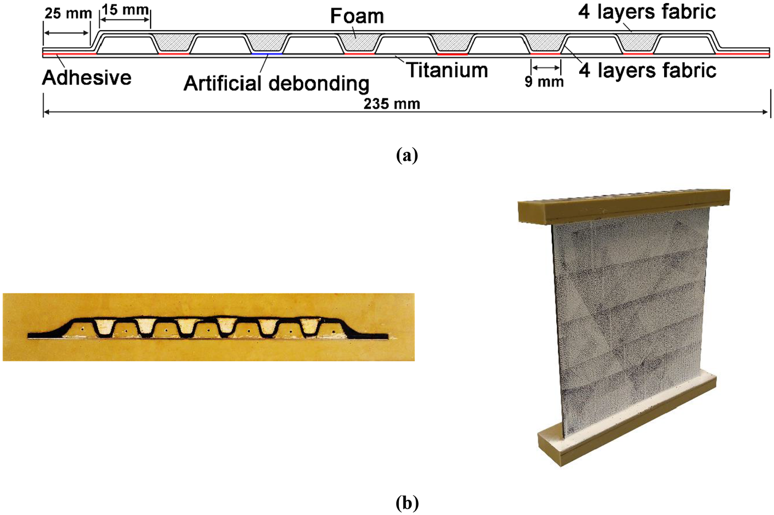
(a) A schematic of the cross-section of the panel and (b) the top and isometric view of the panel.

Figure 2.

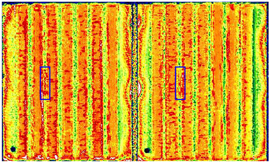
The C-scan image of the two panels. (The artificial debonding is highlighted by a blue rectangle.)

Experiments and characterization

Compression testing

The compression load was applied to the panels by an MTS 3500 kN hydraulic universal tensile/compression machine. The tests were performed under displacement control mode with a rate of 0.2 mm/min. The first test was a monotonic test to determine the maximum load and displacement expected. Then, the second test was a cyclic “loading/unloading” test designed based on the data collected from the monotonic test. The load and displacement values were recorded during the tests by the machine. Four AE sensors were placed on the panel surface, at the positions shown in Figure 3, to record and localize the originated AE signals during the compression test. In addition, DIC system was facing the titanium surface during the loading process to capture the displacement and strain fields on the panel surface. The lateral cross-section of the panel was continuously monitored using a digital camera.

Figure 3.

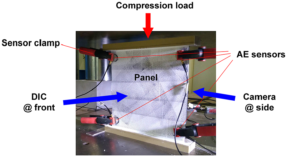
Compression test setup.

DIC

Three-dimensional (3D) DIC system was calibrated and used to capture the displacement contour map during the test. The DIC system, used for the full-field strain measurement, consisted of two 8-bit “Point Grey” cameras with “XENOPLAN 1.4/23” lenses. Both cameras had a resolution of 5 MP. ViC-Snap 8 software was used to record the speckle pattern images with an acquisition rate of 0.33 frames per second (fps) for the monotonic test and 0.25 fps for the cyclic test. Afterward, the acquired images were processed using ViC-3D 8 software. For processing, the subset size was set to 29 pixels with a step size (distance between subsets) of 7 pixels. The observation window of approximately 240 × 230 mm² produced an image with dimensions of 2048 × 1194 pixels.

AE

The AE events of the panel were captured by four AE sensors placed on the panel surface. As shown in Figure 3, the sensors were placed close to the four corners of the panel to get a wider inspection area. The utilized AE sensors are broad-band piezoelectric, AE1045S-VS900M, with an external 34 dB preamplifier. An eight-channel AE system, AMSY-6 (Vallen Systeme GmbH), was employed for the AE measurements. The sampling rate and the threshold were set to 2 MHz and 40 dB, respectively. Ultrasonic gel was applied between the sensor and the panel surface to ensure a good coupling. The pencil lead break procedure³⁴ was performed before the test to check the performance and reproducibility of the AE system.

Particle swarm optimization

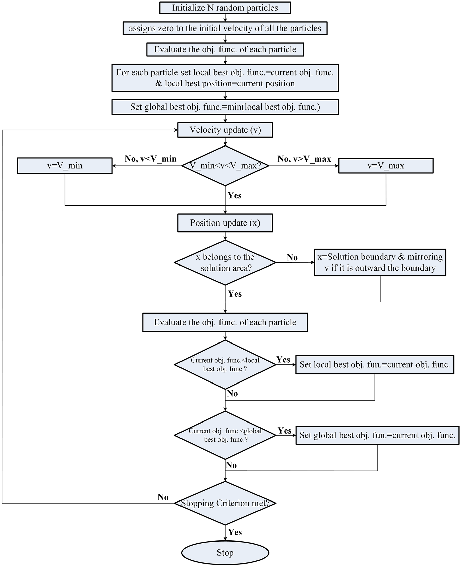
Data clustering can be considered as an optimization process in which an objective function that simultaneously considers similarities of the data points belongs to the same cluster and the dissimilarities of the data points belong to different clusters should be optimized. Some of the frequently used clustering methods for the AE data, such as K-means, fuzzy-c-means, and self-organizing map, may get stuck at a local minimum and do not converge to the best solution, especially for complex datasets.^23,33 Evolutionary algorithms are a kind of population-based random search that is inspired by social behaviors in which the members interact locally with each other and with their environment simultaneously. The main advantage of evolutionary algorithms is the fact that they explore the response space in parallel and in different directions. Therefore, they will less likely be stuck in a local minimum, even for complex datasets. The particle swarm optimization (PSO) is one of the most popular evolutionary algorithms that simulates the social behavior of bird flocking. It is an iterative method to optimize an objective function by moving a population of candidate solutions, particles, in the solution domain by adjusting the position and the velocity of the particles. The movement of each particle is controlled by two factors simultaneously: its local optimum and also the optimum solution found by other particles. In this way, all the particles will gradually move toward the global best solution. Flowchart of the PSO algorithm is depicted in Figure 4. According to the flowchart, the best solution is found in the following steps.³⁵

For a particle i with a position x(i):

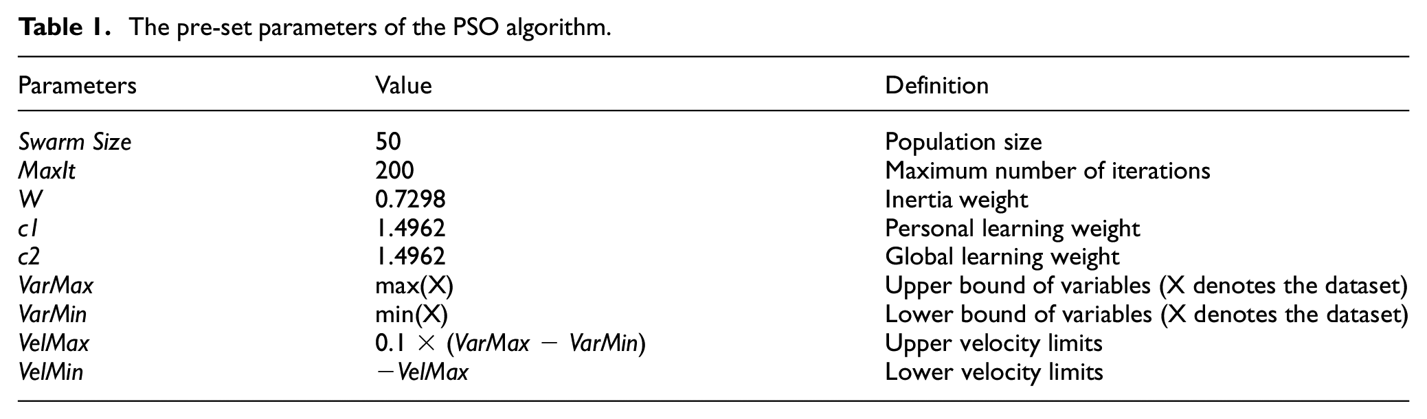
The algorithm creates N random particles, N = Swarm Size, within the variable limits, [VarMin VarMax] (see Table 1).

It assigns zero to the initial velocity of all the particles.

Finding the best objective function among the other particles and the position of that particle ( $g$ ).

Updating the velocity of particle i using equation (1)

v = w \cdot v + c_{1} \cdot r_{1} \cdot (p - x) + c_{2} \cdot r_{2} \cdot (g - x)

(1)

where v is the velocity of particle i. The term (p − x) indicates the difference between the current position and the best position which has been ever found for particle i. The term (g − x) indicates the difference between the current position of particle i and the best position which has been ever found by the other particles. w, c₁, and c₂ are inertia, personal learning, and global learning weight factors, respectively, and r₁ and r₂ are uniformly (0,1) distributed random vectors.

The velocity should be in the predefined velocity limits (see Table 1). If it is lower than VelMin, it is set as VelMin, or if it is larger than VelMax, it is set as VelMax.

The position of particle i is updated as x = x + v.

Checking the interference of the new position of particle i with the solution domain’s boundaries. If it is outside a bound, it is considered equal to that bound, and if its velocity is outside the bound, the velocity is mirrored toward the boundaries.

The objective function is calculated as ( $f = fun (x)$ ).

If the calculated objective function is less than the best objective function which has been ever found by particle i ( $f < fun (p)$ ), then set p = x. This step guarantees that p always represents the best position particle i has had.

In this step, the algorithm calculates the best objective function over the entire particles in the swarm, $b = \min (f (j))$ .

If f < b, then set b = f and d = x, which means b and d are always the best objective function and the best location in the swarm.

If the stopping criterion is satisfied, then algorithm is terminated; otherwise it goes to Step (4). The maximum number of iterations was considered as the stopping criterion in this study.

Table 1.

The pre-set parameters of the PSO algorithm.

Parameters	Value	Definition
Swarm Size	50	Population size
MaxIt	200	Maximum number of iterations
W	0.7298	Inertia weight
c1	1.4962	Personal learning weight
c2	1.4962	Global learning weight
VarMax	max(X)	Upper bound of variables (X denotes the dataset)
VarMin	min(X)	Lower bound of variables (X denotes the dataset)
VelMax	0.1 × (VarMax − VarMin)	Upper velocity limits
VelMin	−VelMax	Lower velocity limits

Figure 4.

Flowchart of the PSO algorithm.

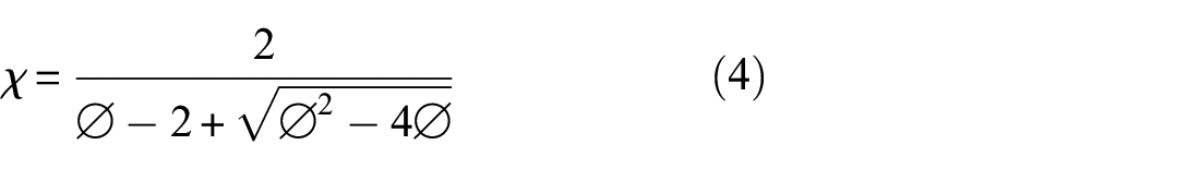
The pre-set parameters of the algorithm used in this study are reported in Table 1. As Clerc and Kennedy³⁶ recommended, if the weight factors of w, c₁, and c₂, are calculated using equations (5)–(7), the best balance between exploration and exploitation throughout the response domain is achieved, which finally leads to the finding of the best solution. Specifically, the best situation is $\emptyset_{1} = \emptyset_{2} = 2.05$ , which consequently leads to $w = 0.7298$ and $c_{1} = c_{2} = 1.4962$ ³⁶

\emptyset_{1}, \emptyset_{2} > 0

(2)

\emptyset = \emptyset_{1} + \emptyset_{2} > 4

(3)

χ = \frac{2}{\emptyset - 2 + \sqrt{\emptyset^{2} - 4 \emptyset}}

(4)

w = χ

(5)

c_{1} = χ \cdot \emptyset_{1}

(6)

c_{2} = χ \cdot \emptyset_{2}

(7)

Results and discussion

Mechanical results

Figure 5 shows the load–displacement curves for the two tested panels, Panel 1 and Panel 2. To obtain the maximum load of the panel, the first panel was subjected to a quasi-static monotonic compression load until the final fracture. As it is depicted in Figure 5, the maximum load of the panel was ∼250 kN. Then, the second panel was subjected to an increasing cyclic load with the load step of 50 kN, including loading, unloading, and then reloading to a higher load level, until the final fracture. The gradient of the load–displacement curve in each loading–unloading cycle is the same until the end of the third load cycle, while, from the fourth load cycle, there is a reduction in the slope of the unloading part in comparison with the loading part of the cycle and a hysteresis area can be seen in the curve. This phenomenon may be attributed to the titanium plastic deformation or damage propagation in the panel. The maximum displacement and failure load are approximately the same for both cases: ∼2 mm and 250 kN, respectively.

Figure 5.

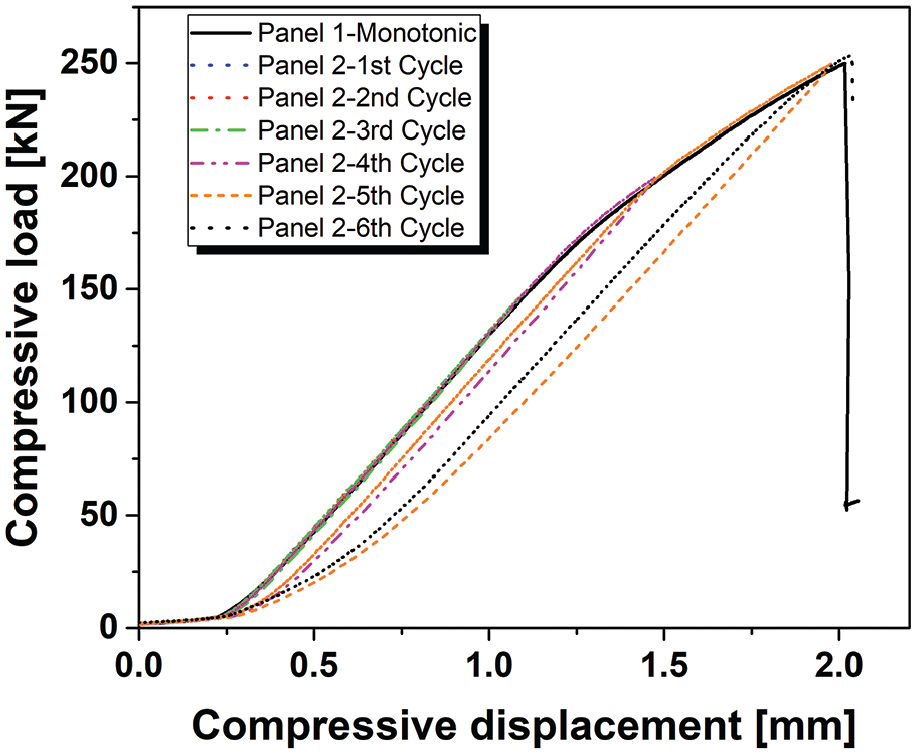
The load–displacement curve of the monotonic and cyclic tests.

In situ monitoring results

In the SHM paradigm, the damage is fully characterized in four levels: damage initiation detection, damage severity, damage localization, and damage type identification. Figure 6 shows the proposed workflow for the damage assessment. Based on the presented workflow, the damage initiation is first detected by means of the cumulative AE curve. Then, in the second level, the damage severity is assessed using the Felicity effect. Afterward, the damage AE signals are localized using the time difference of arrival technique. Finally, the damage type is identified by following several steps which will be fully described in section “Damage mechanisms identification.”

Figure 6.

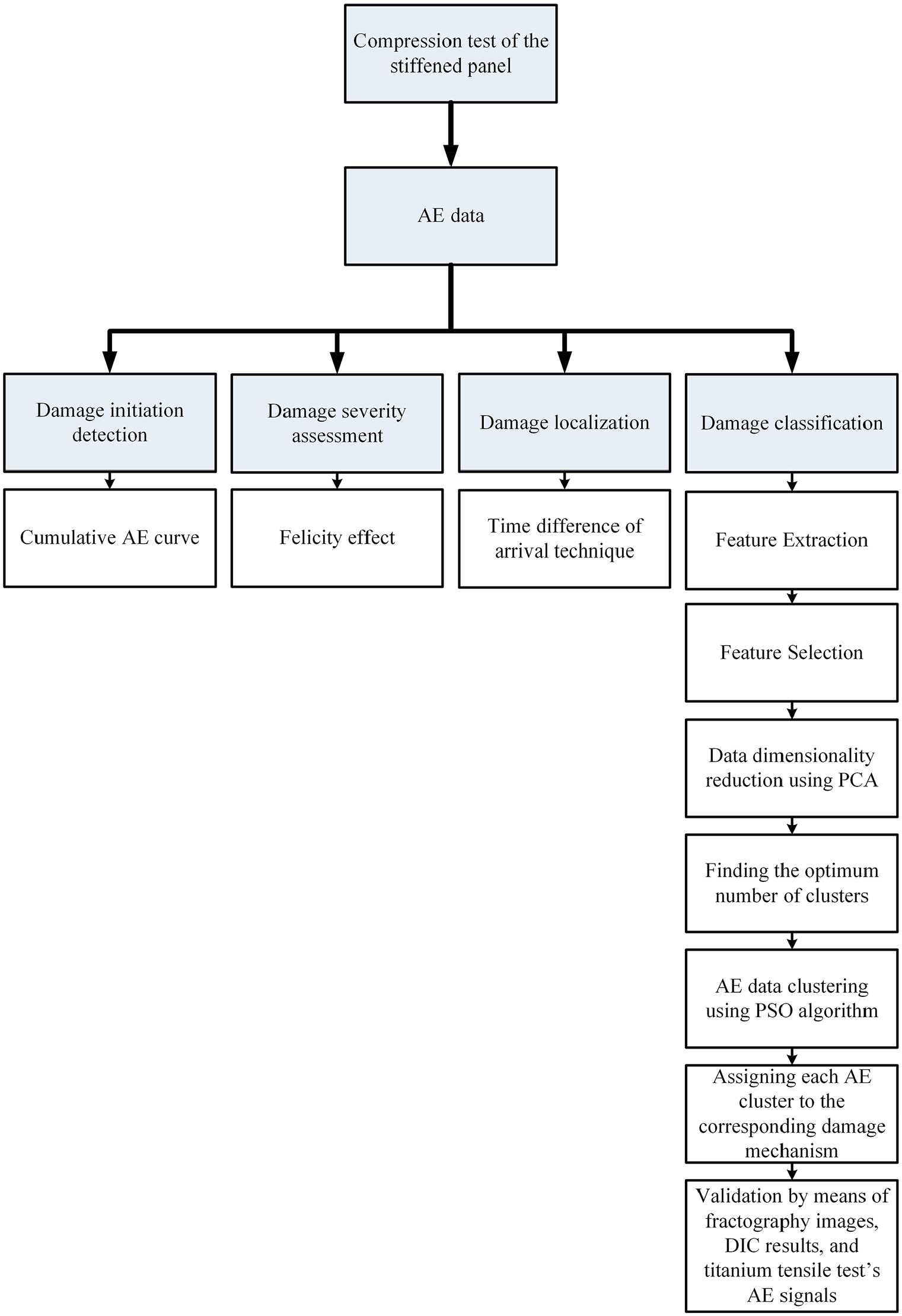
The proposed workflow for damage assessment.

Damage initiation and severity detection

Because of the good consistency between the load–displacement curve of the monotonic and cyclic tests, hereafter, the results are just presented for the cyclic test which easily enables the investigation of the damage evolution in more detail. The cumulative AE events curve during the six load cycles is presented in Figure 7. As it is visible, the first AE event occurred at the end of the third load cycle. In the fourth load cycle, as long as the load is less than the maximum load of the third load cycle, no AE event is detected. Once the load exceeds the maximum load of the third load cycle, a small jump in the cumulative curve occurs. The same trend is observed in the fifth load cycle, that is, no AE event occurs till the load exceeds the maximum load of the previous load cycle. However, at the end of the fifth load cycle, a very significant jump happened, which may indicate a severe damage in the panel as discussed later in this section. Ultimately, at the end of the sixth load cycle, another big jump in the cumulative curve is visible, which corresponds to the final fracture of the panel. The digital camera placed at the lateral side of the panel did not show any debonding or CFRP stringer failure at the edge before the final fracture of the panel which is consistent with the similar results reported in the literature.³⁰

Figure 7.

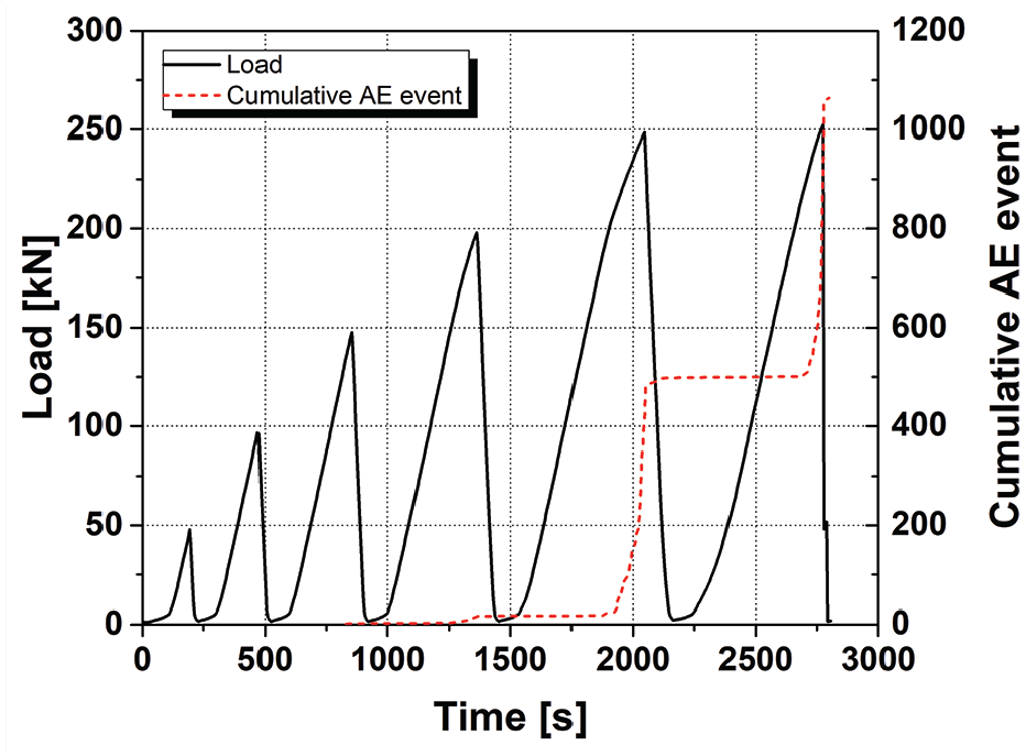
The cumulative AE events during the cyclic test.

For precisely detecting the damage initiation, the Kaiser and Felicity effects^37,38 are used. The Kaiser effect, introduced by Kaiser in the 1950s, is a method for evaluating the damage state in a structure. According to Kaiser’s principle, once a structure is loaded up to a load higher than the damage-inducing threshold, it generates AE events, while if the structure is unloaded and reloaded again, it does not generate AE events anymore until the load crosses the maximum load of the previous cycle. This phenomenon indicates that the structure has not been degraded significantly because of the induced damage. However, in the reloading cycle, if AE events occur at a load level lower than the maximum load of the previous cycle, this is called “Felicity effect.” This indicates that severe/critical damage occurred in the structure which significantly degraded its integrity. To calculate the Kaiser and Felicity effect, in each load cycle, the load corresponding to the initiation of the significant AE activities is divided by the maximum load of the previous load cycle. As long as this ratio is equal to or greater than 1, the Kaiser effect prevails which indicates no critical damage occurrence. When the ratio drops below 1, the Felicity effect prevails which corresponds to considerable damage in the panel. In other words, the Kaiser effect can be considered as a special case of the Felicity effect (when the Felicity effect is 1). It is clear that the lower the value of the Felicity effect, the more the severity of the damage in the structure. Figure 8 depicts the Kaiser and Felicity effects in the cyclic test. Because there is no AE event in the first two cycles, the ratio cannot be defined for them. As it is clear, the ratio for the third, fourth, and fifth load cycles is greater than or equal to 1 which shows the Kaiser effect; however, it drops to ∼0.9 at the beginning of the sixth load cycle, which shows the Felicity effect. Therefore, it indicates that the panel was severely damaged during the fifth load cycle, and this finally led to the catastrophic failure in the sixth load cycle.

Figure 8.

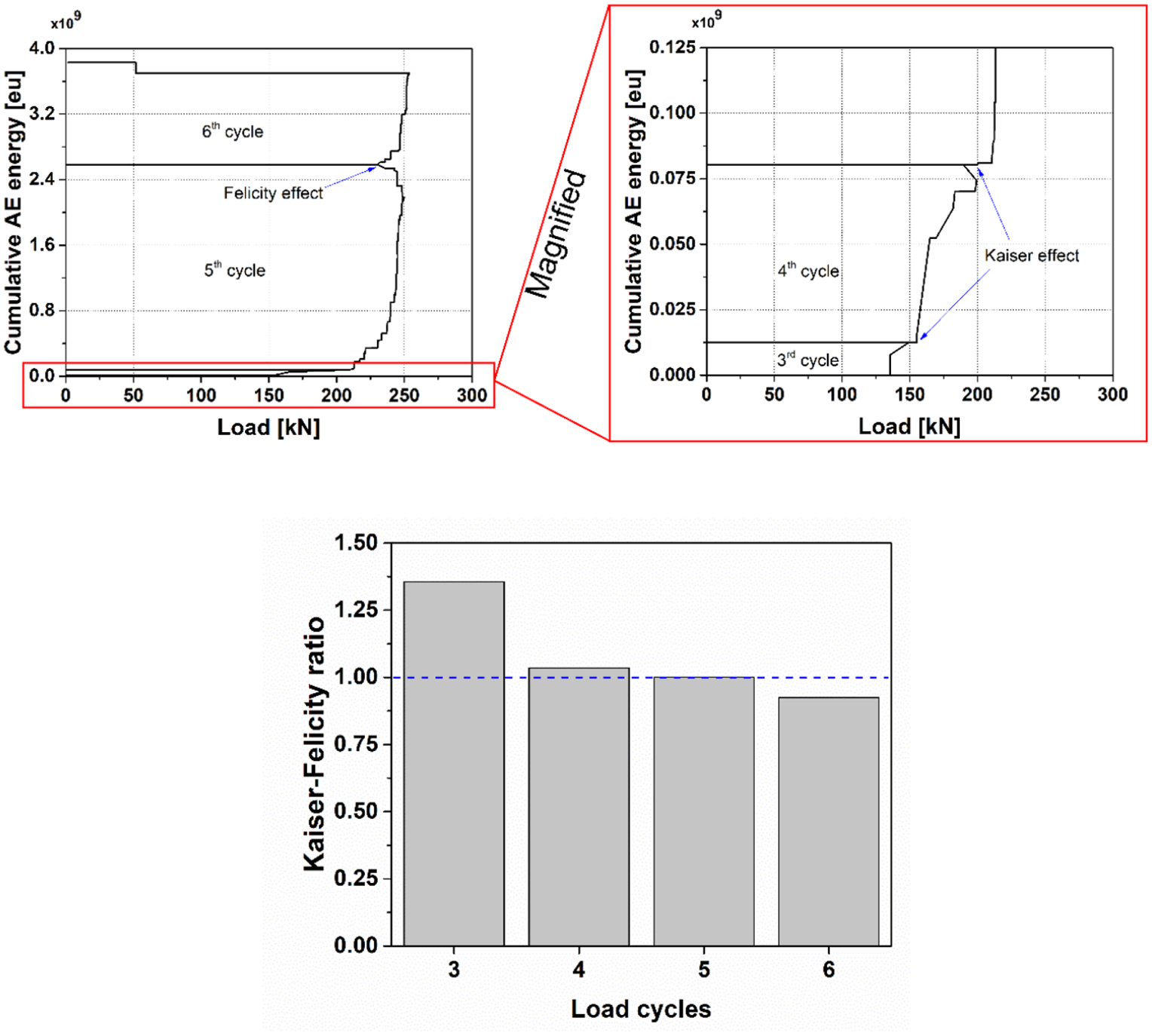
Kaiser and Felicity effects for the cyclic test.

Damage localization

The next stage of the damage characterization is localizing the damage. Thus, the AE events captured by the AE sensors were localized by the time difference of arrival technique.³⁹ To avoid considering the reflected waves from the boundaries as the damage hit, two time-related parameters were considered: (1) first hit discrimination time (FHD) and (2) maximum time difference (MTD) between the first and last hits of the same event. Once, the first hit of a new event is recorded by a sensor, all the hits arriving at the other sensors less than MTD are considered as the same event dataset. By expiring MTD, the events dataset is closed. For a new event, a new dataset is opened and the first hit is recorded, if the time to the previous hit is larger than FHD. An event is localized if at least three out of four sensors record its corresponding hits. In the tested panel, by considering the farthest possible event from one of the AE sensors (the diagonal of the sensor grid in Figure 3 is ∼0.3 m) and the measured wave velocity in the titanium panel (4950 m/s), the MTD of arrival for the farthest sensor from the event source is ∼60 μs (0.3 m over 4950 m/s). Therefore, the MTD was set as 60 μs to avoid considering the reflected waves as the damage hit. In addition, to give enough time to the panel to damp the reflected waves of an event from the boundaries, FHD was set as 1 ms.

The density plot of the localized events is shown in Figure 9. The initial location of the artificial debonding is highlighted by the hatched rectangle. As it is clear, no AE event is detected in the first two cycles. At the end of the third load cycle, the first AE event was localized close to the artificial debonding. Afterward, the density of the AE events considerably increased at the end of the fourth load cycle, and they were mostly located in the vicinity of the artificial debonding. At the end of the fifth load cycle, a new dense-AE events group was localized at the right side of the panel, which indicates the occurrence of a new damage at this region. Finally, in the density plot of the end of the sixth load cycle, another increase in the density function around the artificial debonding was observed, which emphasizes that the damage mostly propagated around the artificial debonding during this load cycle.

Figure 9.

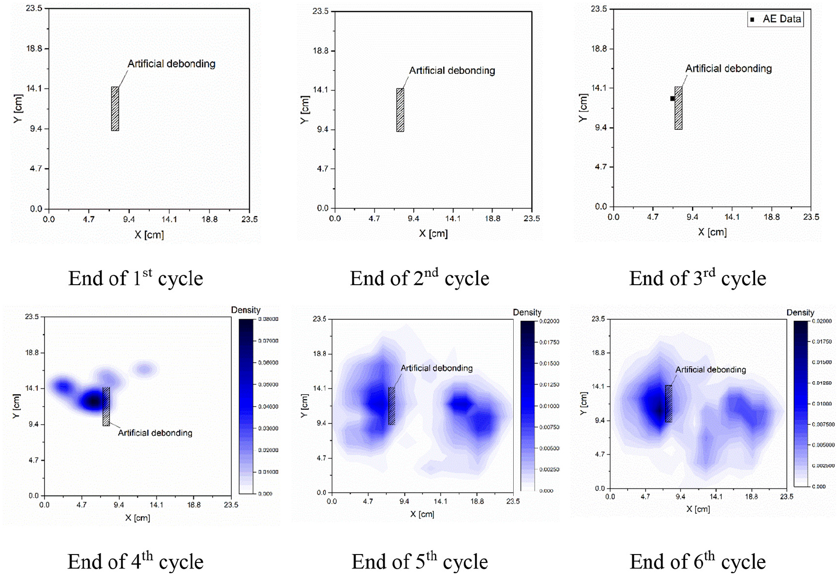
Damage localization by AE at the end of six load cycles (artificial debonding is represented by a hatched rectangle).

To verify the AE localization results, the DIC was also employed to trace the damage evolution in the panel during six load cycles. Figure 10 summarizes the out-of-plane displacement of the titanium panel obtained from DIC. Almost a uniform displacement distribution is observed on the panel’s surface for the first three cycles. Starting from the end of the fourth load cycle, an out-of-plane concentration appeared at the location of the artificial debonding, which is consistent with the AE localization results (see Figure 9). This concentration gets magnified in the fifth load cycle. At the sixth load cycle, another out-of-plane concentration is visible at the right side of the panel, which is in agreement with the AE localization results for the fifth and sixth load cycles. Although the DIC results are consistent with the AE results, it has a one-cycle delay in comparison to AE. This is due to the fact that AE detects the debonding propagation, while the increase in the out-of-plane displacement, which is detected by DIC, is a consequence of this debonding propagation.

Figure 10.

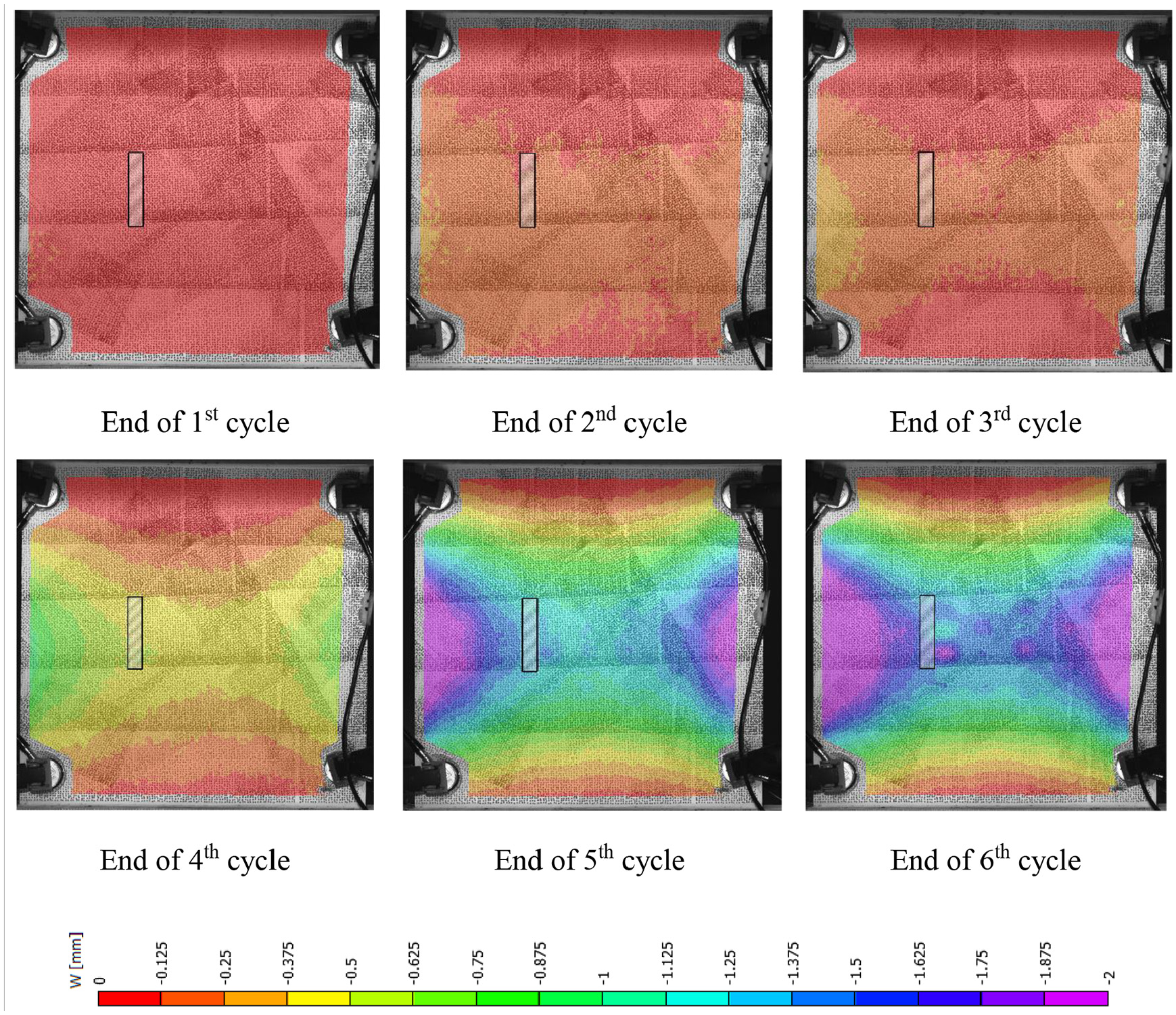
The out-of-plane displacement field at the end of six load cycles obtained from DIC (artificial debonding is illustrated by a hatched rectangle).

Damage mechanisms identification

As depicted in Figure 6, the damage clustering using AE signals is done in seven steps: (1) feature extraction, (2) feature selection, (3) data dimensionality reduction using Principal Component Analysis (PCA), (4) finding the optimum number of clusters, (5) AE data clustering using the PSO algorithm, (6) assigning each AE cluster to the corresponding damage mechanism, and (7) validation of the damage clustering results. The details of each step will be discussed later.

Twelve AE features, which have been mostly used in the literature, were extracted for the AE signals and they are presented in Table 2. The upper and lower limits of the features were specified based on the AE dataset of the cyclic test. In the feature selection step, the features with the highest discriminating capability should be selected among all the available AE features because these features will lead to a larger spread of the data. As it is clear from Table 2, because the features are in different units and also their ranges are completely different, the variation of the raw data is not comparable. Therefore, each feature is first being scaled to a range of [0, 1] by dividing all the feature values by the maximum value of that feature. Then, a descriptive statistical analysis is performed using the box plot. In this way, five main parameters are determined including: the median, the first quartile, the third quartile, and the data min and max. This ensures that all the data are compared with the same confidence interval of 99.3% as depicted in Figure 11. Accordingly, the top five features with the highest discriminating capability, that is A, FFT_CoG, RMS, FFT_FoM, and R/D, are selected for the rest of the analysis.

Figure 11.

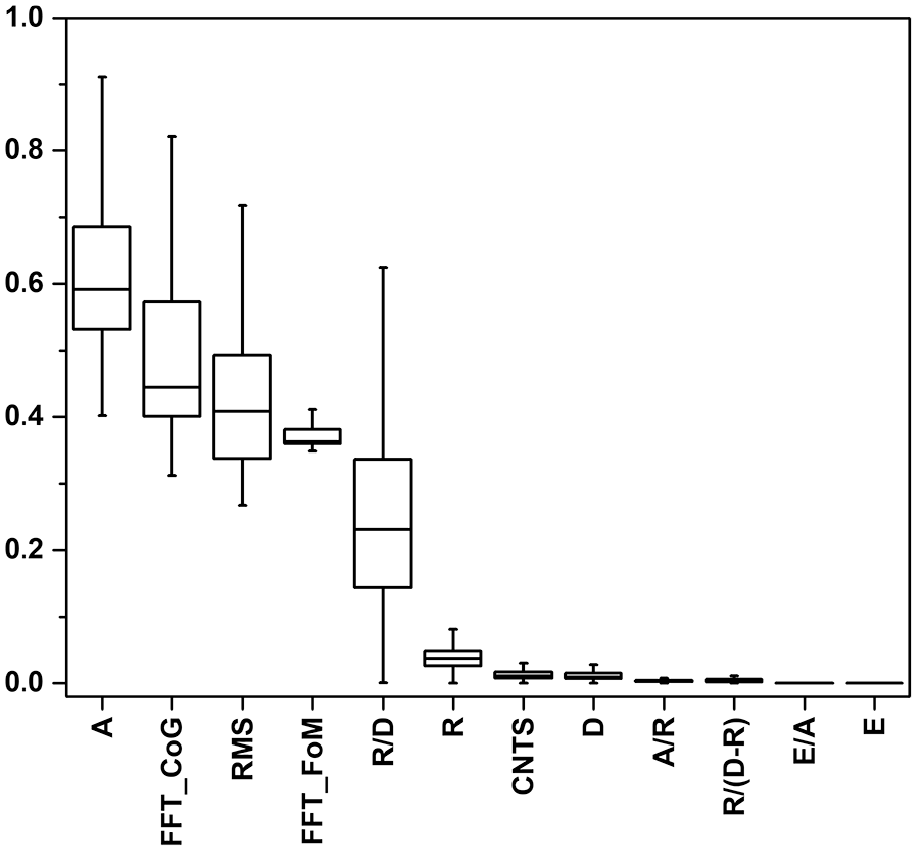
The results of a descriptive statistical analysis for the AE data of the cyclic test.

Table 2.

The specifications of the AE features.

Feature	Symbol	Unit	Lower limit	Upper limit
Amplitude	A	dB	40	100
Rise time	R	µs	0.1	1000
Duration	D	µs	0.1	1000
Energy	E	eu	9	2.6e8
Root mean square	RMS	µV	3.8	14.2
Counts	CNTS	-	0	2790
Rise time/duration	R/D	-	0	0.0005
Energy/amplitude	E/A	eu/dB	0.22	2.64e6
Rise time/(duration−rise time)	R/(D−R)	-	0.0005	91.2
Amplitude/rise time	A/R	dB/µs	0.076	417
Centroid frequency	FFT_CoG	kHz	131.3	420
Peak frequency	FFT_FoM	kHz	125.5	359.9

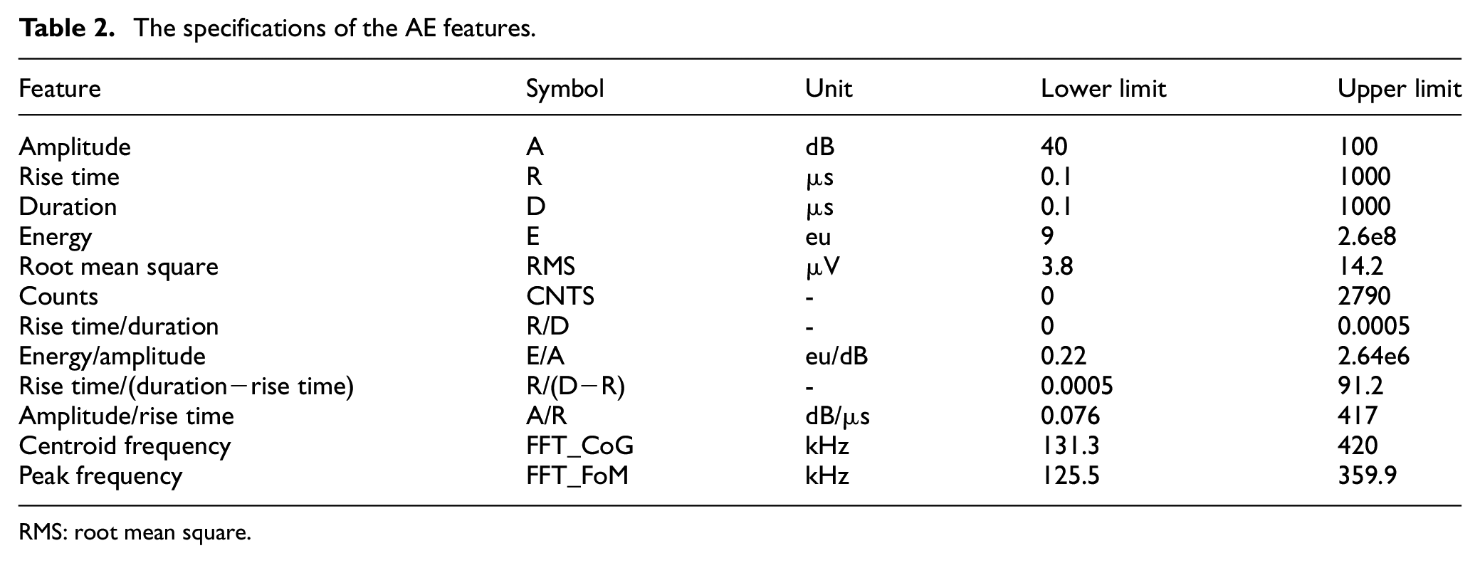
RMS: root mean square.

The five selected features are then analyzed using the PCA method to reduce the dimensionality of the dataset for easier data manipulation and analysis. The PCA creates new independent variables (principal components), made as a linear function of the initial variables, that maximize variance (increasing data discrimination potential). In the PCA, most of the initial variables information will be put in the first components. More details on the PCA method can be found in Pashmforoush et al.⁴⁰ In this study, because the initial data dimensionality was five (five features including A, FFT_CoG, RMS, FFT_FoM, and R/D), PCA resulted in five principal components in which most information is found in the first component, then in the second, and so forth. Figure 12 shows the first two principal components of the AE signals of the panel (PCA 1 and PCA 2) that provide the highest discrimination for the AE dataset.

Figure 12.

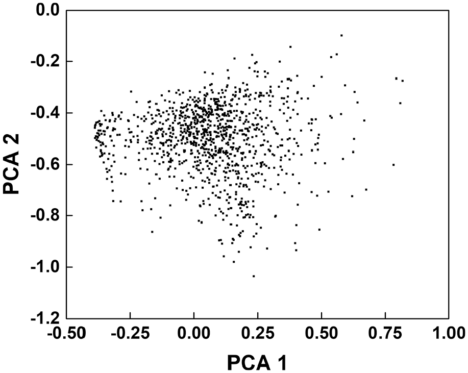
The PCA components for the AE data of the cyclic test.

In the case of supervised classification, the number of classes is known from the training dataset beforehand. On the contrary, in the case of unsupervised clustering, finding the optimum number of clusters is a challenge. Before clustering the data, the optimum number of clusters was obtained using Davies–Bouldin, silhouette, and Calinski–Harabasz criteria. All these three methods find the optimum number of clusters by performing an iterative optimization process. In the case of the Calinski–Harabasz criterion, the objective function is defined as a function of the ratio of the between-cluster variance to the within-cluster variance. The best response would be found in the case of the largest between-cluster variance and the smallest within-cluster variance. In the case of the silhouette criterion, it tries to maximize an objective function that indicates the similarity of one data point to its own cluster. It varies from −1 to +1, in which the higher the value, the better the response. Finally, the Davies–Bouldin criterion almost does the opposite of the Calinski–Harabasz criterion, and its objective function is defined as the ratio of within-cluster to between-cluster distances. Therefore, in this criterion, the lower the value, the better the response. The details of these criteria can be found in Calinski and Harabasz,⁴¹ Davies and Bouldin,⁴² and Rousseeuw.⁴³ In conclusion, the highest value of Calinski–Harabasz and silhouette indices and the lowest value of the Davies–Bouldin index indicate an optimum number of clusters. Therefore, as depicted in Figure 13 for the present AE dataset, the optimum number of clusters for the AE dataset is 4.

Figure 13.

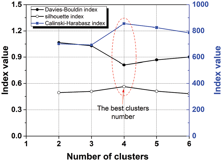
Specifying the best number of clusters using Davies–Bouldin, silhouette, and Calinski–Harabasz indices.

Afterward, the PSO algorithm was used to cluster the AE data into four clusters by minimizing the following objective function (within-cluster distance (WCD))

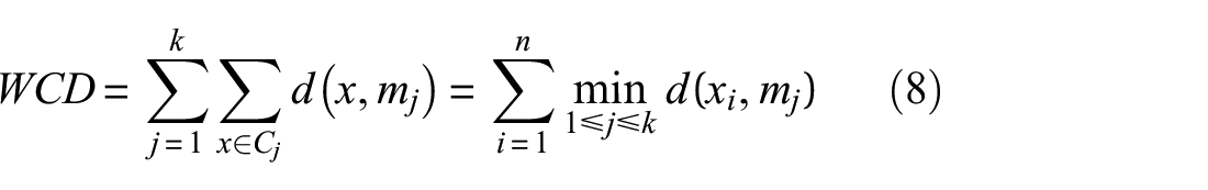
WCD = \sum_{j = 1}^{k} \sum_{x \in C_{j}} d (x, m_{j}) = \sum_{i = 1}^{n} min_{1 \leq j \leq k} d (x_{i}, m_{j})

(8)

where x indicates a data point, k is the number of clusters, C_j is cluster j, m_j represents the centroid of cluster j, d is the Euclidean distance, and n denotes the total number of data. The stopping criterion of the algorithm was the maximum number of iterations, which was set as 200.

The clustered data and the values of the objective function in each iteration are summarized in Figure 14. After ∼30 iterations, the PSO algorithm converged to the best clustering solution.

Figure 14.

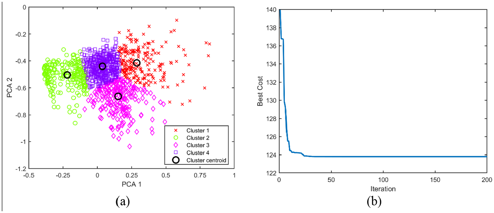
(a) The clustered AE data and (b) the objective function value in different iterations.

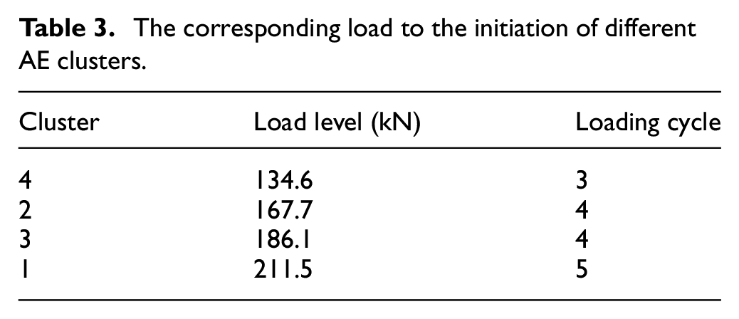
The cumulative number of events for each cluster during the cyclic test is illustrated in Figure 15. The first cluster, which started at the end of the third load cycle, is cluster 4. Then, clusters 2 and 3 initiated at the end of the fourth load cycle. Cluster 1 is the last one starting at the end of the fifth load cycle. The load level corresponding to the initiation of each cluster is reported in Table 3.

Figure 15.

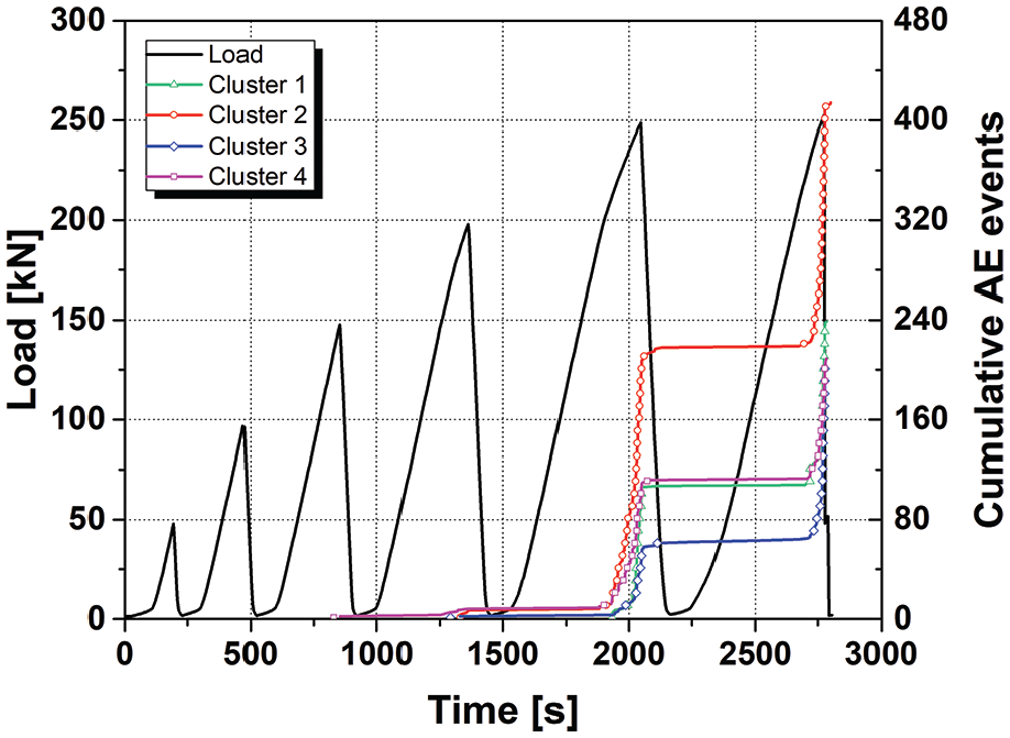
The number of cumulative events for different clusters during the cyclic test.

Table 3.

The corresponding load to the initiation of different AE clusters.

Cluster	Load level (kN)	Loading cycle
4	134.6	3
2	167.7	4
3	186.1	4
1	211.5	5

To correlate these AE clusters to the associated damage mechanisms, first, the clusters were localized. Then, the location of each cluster was compared with the trace of the different damages on the fracture surface of the panel. As shown in Figure 16, cluster 4 was mainly located close to the artificial debonding, while cluster 1 was mostly located at the right side of the panel, far from the artificial debonding. Clusters 2 and 3 were almost distributed in the whole area of the panel. To find the damage mechanisms associated with these clusters, the damaged panel was cut from the region shown in Figure 17(a). The images of the damaged CFRP–titanium interface are depicted in Figure 17(b). The dominant damage mechanism at the left side of the panel, where the artificial debonding exists, is the separation of the adhesive layer from CFRP or titanium, “adhesive failure.” The adhesive material which only remained on one side of the titanium–CFRP interface is an evidence of the adhesive failure, while, at the right side of the panel, the dominant damage mechanism is the damage within the adhesive layer, “cohesive failure.” The trace of the adhesive material on both surfaces of the CFRP and the titanium is a signature of the cohesive failure mode.

Figure 16.

Localization of different AE clusters at the end of the sixth load cycle: (a) cluster 1, (b) cluster 2, (c) cluster 3, and (d) cluster 4 (the artificial debonding is highlighted by a hatched rectangle).

Figure 17.

(a) The cutting lines of the panel and (b) 2D and (c) 3D images from the surface of the CFRP stringers and the titanium panel (adhesive material is visible as green hunks on the fracture surface).

Therefore, the AE cluster 4 which was mainly located at the left side of the panel is correlated to the adhesive failure and cluster 1 which mostly occurred at the right side of the panel is allocated to the cohesive failure. To determine the source of clusters 2 and 3, which were distributed in a wider area, the longitudinal strain of the titanium panel during the six load cycles was calculated by the DIC and it is plotted in Figure 18. According to the titanium datasheet, the yielding strain of the titanium panel is ∼0.25%. From the strain curve of the panel (see Figure 18), it is clear that up till the end of the third load cycle, the strain value is less than the yield strain of the titanium, while in the fourth load cycle, the strain exceeds the titanium’s yielding strain. This moment is almost consistent with the initiation of clusters 2 and 3 in the fourth load cycle in Figure 15. Thus, one or both of clusters 2 and 3 can be attributed to the titanium yielding. To find out the similarity of these two clusters and the titanium yielding signals, the standard dog bone test sample was fabricated out of the titanium panel and it was subjected to the quasi-static tensile test, while its AE activities were recorded by the AE sensor. The similarity_index was defined to calculate the similarity of the titanium yielding signals and clusters 2 and 3

d_{i} = \frac{1}{n_{i} (n_{i} - 1) / 2} \sum_{i = 1}^{n_{i} - 1} \sum_{j = i + 1}^{n_{i}} d (x_{i}, x_{j}); x_{i}, x_{j} \in C_{i}

(9)

d_{o} = \frac{1}{n_{i} n_{j}} \sum_{i = 1}^{n_{i}} \sum_{j = 1}^{n_{j}} d (x_{i}, x_{j}); x_{i} \in C_{i} and x_{j} \in C_{j}

(10)

Similarity_index = \frac{d_{o} - d_{i}}{\max (d_{o}, d_{i})}

(11)

where $C_{i}$ indicates cluster i, $n_{i}$ is the number of data points of cluster i, and $d (x_{i}, x_{j})$ determines the distance between two data points $x_{i}$ and $x_{j}$ . $d_{i}$ indicates the average of internal distances of data points inside cluster i, while $d_{o}$ shows the average of the external distance of data points of cluster i from the other clusters’ data points. Here, $C_{i}$ denotes the titanium yielding AE dataset and $C_{j}$ represents clusters 2 and 3. Each data point, x, was defined by five features, including A, FFT_CoG, RMS, FFT-FoM, and R/D. The similarity_index value of 1 indicates that there is no similarity between the titanium yielding signals and clusters 2 and 3, while an index value close to 0 or even a negative value indicates a huge similarity between the titanium yielding signals and these two clusters. The similarity_index values for clusters 2 and 3 were 0.1441 and 0.0109, respectively, which indicates a high similarity between the titanium yielding signals and both clusters 2 and 3. Therefore, as both clusters started at the same time and also they had a very small similarity_index values with the titanium yielding signals, both clusters 2 and 3 are allocated to the titanium yielding. The camera placed at the side of the panel did not show any damage in the CFRP stringers up to the moment of the final failure of the panel which is consistent with the literature.³⁰ Therefore, no AE cluster is dedicated to the CFRP failure.

Figure 18.

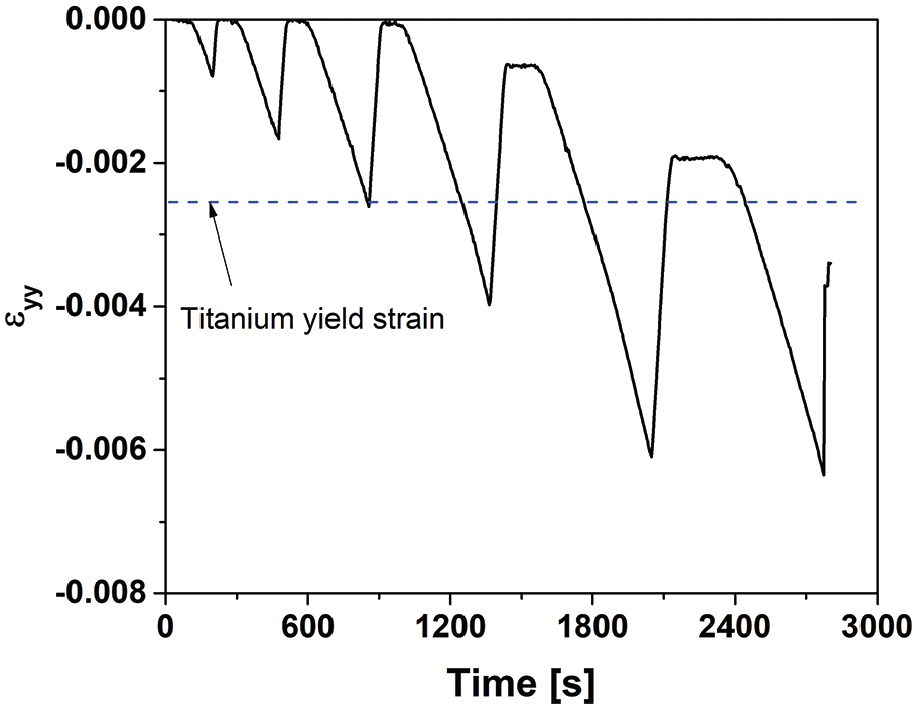
The normal strain on the surface of the titanium panel during the six load cycles obtained from DIC.

In summary, clusters 4 and 1 were allocated to the adhesive failure and cohesive failure, respectively, by mapping the localized clusters to the fractography image of the damaged panel. Regarding clusters 2 and 3, they started simultaneously at the fourth load cycle while the DIC indicated yielding of the titanium panel. Moreover, the proposed similarity index for the AE signals obtained from the tensile test of a titanium sample, from one side, and both clusters 2 and 3, from the other side, revealed a high similarity. Therefore, both clusters 2 and 3 were dedicated to the titanium yielding.

Conclusion

This study was devoted to the SHM of an aeronautical titanium panel stiffened by the omega shape CFRP stringer using AE and DIC techniques. Two panels with a small artificial debonding between the titanium sheet and one of the CFRP stringers were fabricated. The first panel was subjected to a quasi-static monotonic compression load to find the maximum load, which was ∼250 kN, and accordingly, the second one was subjected to an increasing cyclic load with the load step of 50 kN up to final fracture. The AE was used to comprehensively characterize the damage, that is, damage initiation detection, damage severity, damage localization, and damage type identification. The concluding remarks are summarized as follows:

The AE analysis enabled the distinction between the damage initiation and damage severity. Despite the fact that damage initiation occurred at the end of the third cycle, it was not severe enough to affect the integrity of the structure. This was confirmed by the Felicity analysis highlighting the occurrence of the severe damage only at the end of the fifth cycle.

The localized AE events on the panel surface were consistent with the regions with the highest out-of-plane displacement highlighted by DIC. First, the damage started around the artificial debonding and then it propagated to the other side of the panel which resulted in the catastrophic failure of the panel at the end.

Comparing the AE results with the DIC results revealed that although both techniques detected the damage, the DIC detected the damage one cycle later than AE. This is due to the fact that the AE detected the damage propagation, while DIC detected the consequences of this damage, which is the increase in out-of-plane displacement in this case.

Finally, five features with the highest discrimination capability were selected to cluster the AE signals into several clusters using PSO algorithm. The obtained clusters were then assigned to their associated damage mechanisms, that is, adhesive failure, cohesive failure, and titanium yielding.

The obtained results demonstrated the potential of AE, as an SHM technique, for the monitoring of the integrity of the aeronautical composite-to-metal adhesively bonded structures.

Footnotes

Declaration of conflicting interests

The author(s) declared no potential conflicts of interest with respect to the research, authorship, and/or publication of this article.

Funding

The author(s) disclosed receipt of the following financial support for the research, authorship, and/or publication of this article: This research was funded by the Clean Sky 2 Joint Undertaking under the European Union’s Horizon 2020 program TICOAJO (Grant No. 737785).

ORCID iDs

Milad Saeedifar

Mohamed Nasr Saleh

References

Srinivasan

Bertram

. Preliminary design and system considerations for an active hybrid laminar flow control system. Aerospace 2019; 6: 109.

Thielecke

. Methodik zur Leistungsabschätzung von HLFC-Absaugsystemen im Flugzeugvorentwurf. In: Proceedings of the Deutscher Luft- und Raumfahrtkongress (DLRK), Hamburg, 31 August–2 September 2010.

Abramovich

. Test results on stability and vibrations of stringer-stiffened composite panels. In: Abramovich

(ed.) Stability and vibrations of thin walled composite structures. Amsterdam: Elsevier, Ltd, 2017, pp. 575–618.

Arbelo

de Almeida

SFM

Donadon

. An experimental and numerical analysis for the post-buckling behavior of composite shear webs. Compos Struct 2011; 93: 465–473.

Bisagni

Dávila

. Experimental investigation of the postbuckling response and collapse of a single-stringer specimen. Compos Struct 2014; 108: 493–503.

Gal

Levy

Abramovich

, et al. Buckling analysis of composite panels. Compos Struct 2006; 73: 179–185.

Less

Abramovich

. Dynamic buckling of a laminated composite stringer–stiffened cylindrical panel. Compos Part B: Eng 2012; 43: 2348–2358.

Perret

Mistou

Fazzini

, et al. Global behaviour of a composite stiffened panel in buckling. Part 2: experimental investigation. Compos Struct 2012; 94: 376–385.

Stevens

Ricci

Davies

GAO

. Buckling and postbuckling of composite structures. Composites 1995; 26: 189–199.

10.

Williams

Stein

. Buckling behavior and structural efficiency of open-section stiffened composite compression panels. AIAA J 1976; 14: 1618–1626.

11.

Zimmermann

Klein

Kling

. Buckling and postbuckling of stringer stiffened fibre composite curved panels—tests and computations. Compos Struct 2006; 73: 150–161.

12.

De Freitas

Sinke

. Failure analysis of adhesively-bonded skin-to-stiffener joints: metal–metal vs. Composite–metal. Eng Fail Anal 2015; 56: 2–13.

13.

De Freitas

Sinke

. Failure analysis of adhesively-bonded metal-skin-to-composite-stiffener: effect of temperature and cyclic loading. Compos Struct 2017; 166: 27–37.

14.

Kim

Choi

Kweon

. Manufacture and performance evaluation of the composite hat-stiffened panel. Compos Struct 2010; 92: 2276–2284.

15.

. Experiment and optimization of the hat-stringer-stiffened composite panels under axial compression. Compos Part B: Eng 2016; 84: 285–293.

16.

Petersen

Hühne

. Potential of cross section varying Ω stringer made of carbon fibre reinforced plastics. Thin Wall Struct 2016; 103: 253–262.

17.

Zheng

, et al. Damage detection method based on Lamb waves for stiffened composite panels. Compos Struct 2019; 225: 111137.

18.

Memmolo

Monaco

Boffa

, et al. Guided wave propagation and scattering for structural health monitoring of stiffened composites. Compos Struct 2018; 184: 568–580.

19.

Sherafat

Guitel

Quaegebeur

, et al. Structural health monitoring of a composite skin-stringer assembly using within-the-bond strategy of guided wave propagation. Mater Design 2016; 90: 787–794.

20.

Tan

Guan

, et al. Experimental study on effect of impact locations on damage formation and compression behavior of stiffened composite panels with L-shaped stiffener. Thin Wall Struct 2020; 150: 106707.

21.

Ricci

Monaco

Maio

, et al. Guided waves in a stiffened composite laminate with a delamination. Struct Health Monit 2016; 15: 351–358.

22.

Yue

Aliabadi

. A scalable data-driven approach to temperature baseline reconstruction for guided wave structural health monitoring of anisotropic carbon-fibre-reinforced polymer structures. Struct Health Monit 2019; 19: 1487–1506.

23.

Saeedifar

Zarouchas

. Damage characterization of laminated composites using acoustic emission: a review. Compos Part B: Eng 2020; 195: 108039.

24.

Saeedifar

Saleh

De Freitas

, et al. Damage characterization of adhesively-bonded Bi-material joints using acoustic emission. Compos Part B: Eng 2019; 176: 107356.

25.

Andrew

Arumugam

Ramesh

. Acoustic emission characterization of local bending behavior for adhesively bonded hybrid external patch repaired glass/epoxy composite laminates. Struct Health Monit 2018; 18: 739–756.

26.

Haile

Bordick

Riddick

. Distributed acoustic emission sensing for large complex air structures. Struct Health Monit 2017; 17: 624–634.

27.

Zhao

W-Z

Zhou

. Cluster analysis of acoustic emission signals and tensile properties of carbon/glass fiber–reinforced hybrid composites. Struct Health Monit 2019; 18: 1686–1697.

28.

Saleh

Saeedifar

Zarouchas

, et al. Stress analysis of double-lap bi-material joints bonded with thick adhesive. Int J Adhes Adhes 2020; 97: 102480.

29.

Fotouhi

Saeedifar

Sadeghi

, et al. Investigation of the damage mechanisms for mode I delamination growth in foam core sandwich composites using acoustic emission. Struct Health Monit 2015; 14: 265–280.

30.

Dávila

Bisagni

. Fatigue life and damage tolerance of postbuckled composite stiffened structures with initial delamination. Compos Struct 2017; 161: 73–84.

31.

Vanniamparambil

Carmi

Khan

, et al. An active–passive acoustics approach for bond-line condition monitoring in aerospace skin stiffener panels. Aerosp Sci Technol 2015; 43: 289–300.

32.

Kolanu

Raju

Ramji

. Experimental and numerical studies on the buckling and post-buckling behavior of single blade-stiffened CFRP panels. Compos Struct 2018; 196: 135–154.

33.

Sawan

Walter

Marquette

. Unsupervised learning for classification of acoustic emission events from tensile and bending experiments with open-hole carbon fiber composite samples. Compos Sci Technol 2015; 107: 89–97.

34.

ASTM E976-10:2010. Standard guide for determining the reproducibility of acoustic emission sensor response (West Conshohocken, PA: ASTM International, 2010).

35.

Kennedy

Eberhart

. Particle swarm optimization. In: Proceedings of the international conference on neural networks (ICNN’95), Perth, WA, Australia, 27 November–1 December 1995, vol. 4, pp. 1942–1948. New York: IEEE.

36.

Clerc

Kennedy

. The particle swarm—explosion, stability, and convergence in a multidimensional complex space. IEEE T Evolut Comput 2002; 6: 58–73.

37.

Kaiser

. Erkenntnisse und Folgerungen aus der Messung von Geräuschen bei Zugbeanspruchung von metallischen Werkstoffen. Arch Eisenhüttenwes 1953; 24: 43–45.

38.

Nordlund

. Experimental verification of the Kaiser effect in rocks. Rock Mech Rock Eng 1993; 26: 333–351.

39.

Roberts

. TDOA localization technique. In: Proceedings of the IEEE P80215 working group for wireless personal area networks (WPANs), 2004. New York: IEEE, https://www.enriquedans.com/wp-content/uploads/2013/03/TDOA-localization-techniques.pdf

40.

Pashmforoush

Khamedi

Fotouhi

, et al. Damage classification of sandwich composites using acoustic emission technique and k-means genetic algorithm. J Nondestruct Eval 2014; 33: 481–492.

41.

Calinski

Harabasz

. A dendrite method for cluster analysis. Commun Stat 1974; 3: 1–27.

42.

Davies

Bouldin

. A cluster separation measure. IEEE T Pattern Anal 1979; 1: 224–227.

43.

Rousseeuw

. Silhouettes: a graphical aid to the interpretation and validation of cluster analysis. J Comput Appl Math 1987; 20: 53–65.

Damage assessment of a titanium skin adhesively bonded to carbon fiber–reinforced plastic omega stringers using acoustic emission

Abstract

Keywords

Introduction

Materials and manufacturing

Experiments and characterization

Compression testing

DIC

AE

Particle swarm optimization

Results and discussion

Mechanical results

In situ monitoring results

Damage initiation and severity detection

Damage localization

Damage mechanisms identification

Conclusion

Footnotes

Declaration of conflicting interests

Funding

ORCID iDs

References