Sage Journals: Discover world-class research

Abstract

This article presents a novel transfer learning approach for evaluating structural conditions of rail in a progressive manner, by using acoustic emission monitoring data and knowledge transferred from an acoustic-related database. Specifically, the low-level layers of a model pre-trained on large audio data are leveraged in our model for feature extraction. Compared with conventional transfer learning approaches that transfer knowledge from models pre-trained on normal images, the proposed approach can handle acoustic emission spectrograms more naturally in terms of both data inner properties and the way of data intaking. The training and testing data used for rail condition evaluation contains two months of acoustic emission recordings, which were acquired from an in situ operating rail turnout with an integrated acoustic emission –based monitoring system. Results show that the evolving stages of rail from intact to critically cracked are successfully revealed using the proposed approach with excellent prediction accuracy and high computation efficiency. More importantly, the study quantitatively shows that audio source data are more relevant to the acoustic emission monitoring data than Image data, by introducing a maximum mean discrepancy metric, and the transfer learning model with smaller maximum mean discrepancy does lead to better performance. As a by-product of the study, it has also been found that the features extracted by the proposed transfer learning model (“bottleneck” features) already exhibit a clustering trend corresponding to the evolving stages of rail conditions even in the training process before any label is annotated, indicating the potential unsupervised learning capability of the proposed approach. Through the study, it is suggested that selecting source data more correspondingly and flexibly would maximize the benefit of transfer learning in structural health monitoring area when facing heterogenous monitoring data under varying practical scenarios.

Keywords

Acoustic emission structural health monitoring railway system deep learning transfer learning maximum mean discrepancy audio classification

Introduction

Acoustic emission (AE) is the radiation of acoustic (elastic) waves in solids and occurs when a material undergoes irreversible changes in its internal structure, such as crack expansion or plastic deformation due to aging, temperature gradients, or external mechanical forces. In addition, some other processes that are reversible, such as friction and impact, can also emit AE. Structural changes subject to mechanical loadings are localized sources of elastic waves, which are generated when the accumulated elastic energy reaches the threshold and is rapidly released. Based on this principle, AE-based techniques have been used in various scenarios from locating the event source to evaluating the inner conditions of structures.¹

In railway systems, non-destructive evaluation (NDE) techniques, such as eddy current detection,² magnetic induction tests,³ ultrasonic tests,^4,5 guided wave detection,^6–8 non-contact ultrasonic inspection,^9,10 and alternating current field measurement,¹¹ are extensively used for regular inspection. Most NDE techniques have to be conducted offline to avoid interrupting normal rail service while getting to know the real-time conditions of rail infrastructure is one of the top concerns among rail operators and researchers. There are also some methods that utilize axle box accelerations from onboard monitoring systems to identify singular track defects such as squarts¹² and bolt tightness of fish-plated joints¹³ or to detect rail corrugation.¹⁴ Although these methods can cover a long distance, there may be a long interval between the inspections for a specific location. In contrast, AE-based techniques, as a type of passive inspection methods, enable online monitoring of rail conditions by capturing the sudden energy release due to wheel–rail interactions or crack expansion in rail tracks.^15–17 The applicability of AE for online monitoring of rail crack progression was demonstrated in laboratory tests on rail segments carried out under normal load.¹⁸ In previous research work done by the authors, an AE-based online monitoring system had been developed for rail turnout crack detection. Pilot lab investigations and test line experiments proved the effectiveness of the system in detecting AE bursts generated from abrupt crack expansion.¹⁹ The system was then implemented in an operating freight line and had been taking AE recordings over a long period. However, unlike results from the lab environment, the AE signals acquired under in situ circumstances are often accompanied by other signals including mechanical vibrations and broadband noises induced by intense wheel–rail interactions (especially wheel–rail creepage). These vibrations and noises obscure the crack-induced AE signatures of interest. As demonstrated in authors’ previous research work, for damage detection purpose, conventional time–frequency methods (e.g. power spectrum density (PSD) analysis, wavelet analysis) are able to identify large rail cracks before fractures at the point rail;^19,20 while detection of smaller cracks or damages may refer to a frequency domain Structural Health Index (SHI) updated under a Bayesian framework.²¹ However, beyond damage detection, rail operators are keener on the condition evolvement of rail structures over a period of time before significant cracks literally take place, but both methods cannot well reveal the structural health conditions of rail tracks in a progressive manner using the AE data and are not sensitive enough to identify the early stages of rail deterioration when micro cracks are initializing. Yet, micro fatigue cracks or subtle structural changes at early stages would also generate tiny AE bursts subject to train impacts, and implicitly influence the time–frequency spectrogram with hidden features. However, AE bursts are distributed in a wide frequency band depending on different sizes, orientations, and distributions of the early-stage micro cracks as well as different rail operating environment. Therefore, the optimal damage-sensitive features can be varying from case to case and it is often time-consuming to manually extract the optimal one. In light of this, advancement from semi-auto damage detection to automatic online condition evaluation is one target of this study, and deep learning (DL), in this sense, would be a promising option to adaptively find out the features and realize the target.

DL models learn nonlinear representations that disentangle different underlying factors of variation.^22,23 Conventional methods requiring manually analyzing signals or proposing health-relevant features. For example, component analysis was performed to extract AE features, which were then fed to a multi-class relevance vector machine to extract and identify various types of defect bearings.²⁴ The study in Pandya et al.²⁵ manually extracted statistical and acoustic features by Hilbert–Huang transform and then used K-nearest neighbor algorithm to classify five bearing conditions. In comparison, DL can directly map the acquired raw data to the targets, and thus prevent subjective judgments or labor-intensive feature handcrafting. Thus, DL-based approaches have been gradually introduced to structural health monitoring (SHM) in recent years.^26,27 Among the DL models, convolutional neural networks (CNNs), through the hierarchical architecture consisting of multiple convolutional and pooling layers, are able to capture robust representations of a given image.²⁸ For audio data, CNNs also exhibit their capability of digging out suitable salient features that typically outperform handcrafted features in a variety of scenarios including acoustic event detection²⁹ and music onset detection.³⁰ It is also possible to diagnose faults of roller bearings using acoustic recordings and CNN model.³¹ The good performance of CNNs in audio recognition promotes their application in AE-based monitoring. For fault diagnosis of mechanical systems, the diagnostic accuracy can be enhanced by fusing the vibration signals with AE signals³² and integrating CNNs with another kind of network.³³ For plate-like structures, the reflections and reverberations generated by irregular geometric features may hinder the performance of AE source location. This drawback was overcome by some recent work in the study by Ebrahimkhanlou and colleagues^34,35 that leveraged the power of DL (specifically, stacked autoencoders) of capturing complex patterns. Regarding the monitoring of railway systems, a CNN model was formulated to classify the rail state based on the AE signals collected by tensile testing machines, which involved the probability analysis of multiple AE events to improve the classification performance.³⁶ CNNs were also used to identify three mechanisms that induce AE in the railway field: operational noise, impact, and crack propagation.³⁷ Bayesian optimization was utilized to tune the hyper-parameters and transfer learning (TL) was involved to improve efficiency.

DL relies on large datasets to discover the complex relationship between the raw data and the desired output.²² However, the amount of monitoring data collected from engineering field scenarios, for example., AE data from the rail turnout in this study, is often relatively limited (normally hundreds or thousands of data sequences) and not sufficiently “large” for a “deep” learning process. For example, the study by Li et al.³⁷ had to mix up both field and lab data to handle the data insufficiency of crack propagation-induced AE waves. When the signature of interest caused by structural damage is altered, the DL model may suffer from the overfitting issue and fail to separate factors of variation. This issue is particularly obvious and tricky for rail circumstances where the structural and operating conditions are remarkably different under various open environment. To compensate for the data insufficiency, there has been some limited but pioneering research work in DL-based SHM by introducing TL as a novel improvement of conventional DL methods that learn from scratch. For a typical CNN structure, the low-level layers trained on a large database (e.g. ImageNet) have learned to extract low-level features such as edges, corners, and shapes, which can be shared across tasks.³⁸ Therefore, they can be frozen and transferred to a new model and only the high-level layers need to be fine-tuned using the data of interest. In this way, sufficient data can be guaranteed for new model training, and the training process is dramatically accelerated. Specifically, for civil infrastructures, a pioneering study has been conducted on TL-aided SHM,³⁹ in which a relatively small number of images (2000) about structural damages were available. The low-level layers of VGGNet,⁴⁰ which had been pre-trained on a large-scale off-the-shelf dataset named ImageNet⁴¹ containing more than 1000 types of objects, were utilized for extracting features from structural damage images for four structural damage recognition tasks: component type identification, spalling condition check, crack level evaluation, and damage type determination. In a population-based SHM scenario,⁴² three kinds of TL approaches were used so that models trained on the labeled feature data obtained from one structure can be applied to the unlabeled data of a different structure.

For AE-based SHM cases, there has been a very recent work that utilizes TL.³⁷ This study leverages the low-level layers of a model pre-trained on images (Alexnet) to extract features from the time–frequency wavelet spectrograms. This practice, however, has one limitation: AE spectrograms (in target domain) and natural images (in source domain) are not analogous to each other in nature. An AE spectrogram is the time–frequency representation of acoustic waves and not necessarily exhibits edges, corners, or shapes, which appear in an image presenting the spatial distribution of electromagnetic wave frequency. Thus, it is crude and questionable to utilize image-oriented models for spectrograms of AE. The data insufficiency issue mentioned in the previous paragraph could have been overcome if a more reasonable source domain was selected. After all, when the source domain and target domain are more related, less amount of data are required and fewer layers need to be fine-tuned.²⁸ In contrast, each crack-induced AE burst can be considered as an acoustic event and a segment of online audio recording also contains one or multiple acoustic events. Thus, online audio databases that contain various kinds of sound events can be a good alternative source, based on which our “acoustic-homologous” approach is proposed. This is the second and core objective of the study.

This article presents a TL approach to evaluate the rail condition in a progressive manner with AE monitoring data and a large-scale online audio database AudioSet. The AE monitoring data were acquired by an AE-based monitoring system previously developed by the authors and implemented on an operating rail freight line. The low-level layers of the CNN model leverage knowledge transferred from AudioSet, and the remaining layers of the model are trained on AE monitoring data for condition assessment of the rail structure. To the authors’ knowledge, it is for the first time pre-trained model from audio database rather than image database is adopted to more precisely extract the acoustic-specific features of our AE monitoring data. Furthermore, a maximum mean discrepancy (MMD) metric is introduced to quantitatively measure the relevancy between different source data (AudioSet, ImageNet) and target data. The effectiveness of the proposed approach is demonstrated by comparing the performance of the developed network (N_A-AE) with two baselines: one network (N_I-AE) relies on the knowledge from ImageNet in VGGNet, another network (N_AE) is learned from scratch without the involvement of TL. This study stresses the importance of data source selection correspondingly in TL-aided SHM, which can be highly beneficial when facing various types of SHM data.

The organization of this article is as follows: The section “TL and MMD” briefly introduces the basic principles of TL and the concept of MMD; the section “In-situ AE-based monitoring system” describes in detail the in situ AE-based monitoring system and AE monitoring data used for this study; the section “Methodologies” presents the detailed procedures of the proposed approach and the methodologies to validate its effectiveness; the section “Results and discussion” demonstrates and discusses the results; and the section “Conclusion and future work” summarizes the article with conclusions and future work.

TL and MMD

This section introduces the basic principles of TL and the concept of MMD in the context of supervised DL. Given a dataset ${X, Y}$ , $X = {x_{1}, x_{2}, \dots, x_{n}} \in X$ contains n samples and $Y = {y_{1}, y_{2}, \dots, y_{n}} \in Y$ consists of their corresponding label. The task of supervised learning is to learn a model to map x to y or a conditional probability distribution $P (Y | X)$ . The space $X$ and the marginal probability distribution $P (X)$ constitute a domain $D = {X, P (X)}$ and the task is denoted as $T$ .

Unlike conventional machine learning (ML) approaches that require preliminary hand-crafting features from x, DL models can directly map the acquired data x in its raw form to the desired output y.²² The process of feature extraction is embedded in the model. A typical DL model, such as a CNN, consists of a series of layers. Each layer intakes the output of its previous layer, conducts some operations and outputs the features. Each output is a more abstract representation of the original input. It should be noted that lower the level of a layer, less task-specific it is.²⁸ For example, the low-level layers in a CNN can only detect edges and corners in an image, while the high-level layers can output the feature maps that indicate the existence and location of shapes or objects. This finding motives the application of TL in DL applications to increase efficiency and prevent overfitting.

Technically, there has been some knowledge learned from the source domain $D_{S} = {X_{S}, P (X_{S})}$ for the source task $T_{S}$ , and the purpose of TL is to leverage this knowledge to handle the target task $T_{T}$ with the data from the target domain $D_{T} = {X_{T}, P (X_{T})}$ .⁴³ Specifically, the low-level layers of models pre-trained from a large database in $D_{S}$ have learned to extract some low-level features, which are not specific for $T_{S}$ . Therefore, these layers constitute a general feature exactor with well-trained parameters, which can be transferred to other models. Only the high-level layers need to be re-trained on the data of interest in $D_{T}$ for $T_{T}$ .³⁸ This kind of TL is called “parameter-based TL.”

The feature extractor can be approximately shared as long as the $D_{S}$ and $D_{T}$ are sufficiently close. In contrast, if $P (X_{S})$ is too discrepant from $P (X_{T})$ , the feature extractor suitable for $X_{S}$ may not be useful for $X_{T}$ , and sometimes even corrupt $X_{T}$ and reduce the overall performance on the $T_{T}$ .^44,45 Therefore, it is critical to evaluate the discrepancy between $P (X_{S})$ and $P (X_{T})$ , which can be measured quantitatively by some metrics in addition to being intuitively evaluated. One may adopt correlation coefficient (CC) as a more concise metric, but CC only quantifies relevance between two isolated signals/waveforms and cannot truly reflect the closeness of inherent properties (homology) between two domains of data from a more overall perspective. In this study, a non-parametric distance estimate between distributions named MMD⁴⁶ is used. The biggest merit of MMD is that it can quantify the discrepancy between distributions of high-dimensional elements, making it highly suitable for our case.

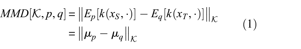
Basically, MMD is a concept in functional analysis defined by the distance between Kernel embedding of two distributions in the reproducing kernel Hilbert space (RKHS) $K$ .⁴⁷ The illustration is shown in Figure 1. A source domain dataset $X_{S} = {x_{s, i}}_{i = 1}^{m}$ and a target domain dataset $X_{T} = {x_{t, i}}_{i = 1}^{n}$ in space $X$ follow the probability distribution p and q, respectively. For a kernel function $k (x, y)$ , $k (x, \cdot)$ represents an implicit way to map a sample x to the RKHS $K$ . When all samples are embedded to the $K$ , the expectation $E [k (x, \cdot)]$ is named “the kernel embedding of distribution” and MMD is defined as

\begin{matrix} MMD [K, p, q] = ‖ E_{p} [k (x_{S}, \cdot)] - E_{q} [k (x_{T}, \cdot)] ‖_{K} \\ = ‖ μ_{p} - μ_{q} ‖_{K} \end{matrix}

(1)

Figure 1.

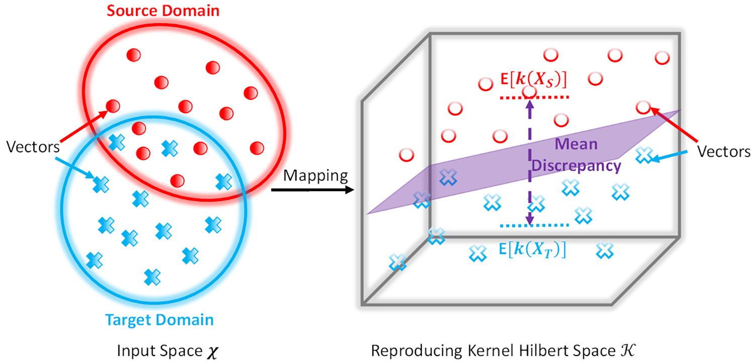
Mean discrepancy between source domain and target domain.

The inner products of embedding samples can be simply calculated by the kernel trick $k (x, \cdot), k {(y, \cdot)}_{K} = k (x, y)$ .⁴⁸ Therefore

\begin{matrix} M M D^{2} [K, p, q] = {‖ μ_{p} - μ_{q} ‖}_{K}^{2} \\ = {〈 μ_{p} - μ_{q}, μ_{p} - μ_{q} 〉}_{K} \\ = {〈 μ_{p}, μ_{p} 〉}_{K} + {〈 μ_{q}, μ_{q} 〉}_{K} - 2 {〈 μ_{p}, μ_{q} 〉}_{K} \\ = E_{p} [{〈 k (x_{S}, \cdot), k ({x^{'}}_{S}, \cdot) 〉}_{K}] \\ + E_{q} [{〈 k (x_{T}, \cdot), k ({x^{'}}_{T}, \cdot) 〉}_{K}] \\ - 2 - 2 E_{p, q} [{〈 k (x_{S}, \cdot), k (x_{T}, \cdot) 〉}_{K}] \\ = E_{p} [k (x_{S}, {x^{'}}_{S})] + E_{q} [k (x_{T}, {x^{'}}_{T})] - 2 E_{p, q} [k (x_{s}, x_{T})] \end{matrix}

(2)

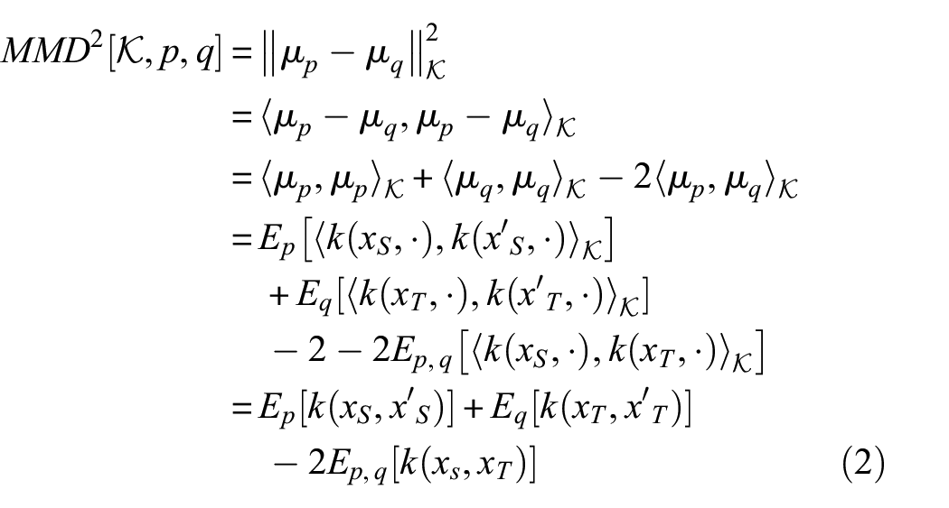
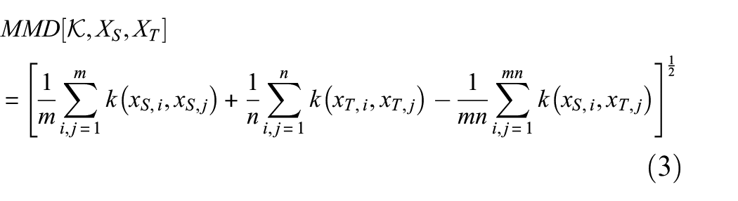
Finally, the empirical estimate based on $X_{S}$ and $X_{T}$ is

\begin{matrix} MMD [K, X_{S}, X_{T}] \\ = {[\frac{1}{m} \sum_{i, j = 1}^{m} k (x_{S, i}, x_{S, j}) + \frac{1}{n} \sum_{i, j = 1}^{n} k (x_{T, i}, x_{T, j}) - \frac{1}{mn} \sum_{i, j = 1}^{mn} k (x_{S, i}, x_{T, j})]}^{\frac{1}{2}} \end{matrix}

(3)

As a non-parametric estimate, MMD does not require an intermediate density estimate, unlike other metrics such as the Kullback–Leibler (KL) divergence. Besides, KL divergence is mainly used to determine information loss rather than discrepancy. To map the terms of TL and MMD into the AE-based SHM case of this study, $D_{T}$ refers to the collection of AE monitoring data and $T_{T}$ refers to our rail condition evaluation task, both of which will be introduced in the section “In situ AE-based monitoring system.” The full construction of the “acoustic-homologous” TL approach will be introduced in the section “Methodologies” with details of MMD calculation.

In-situ AE-based monitoring system

Monitoring system

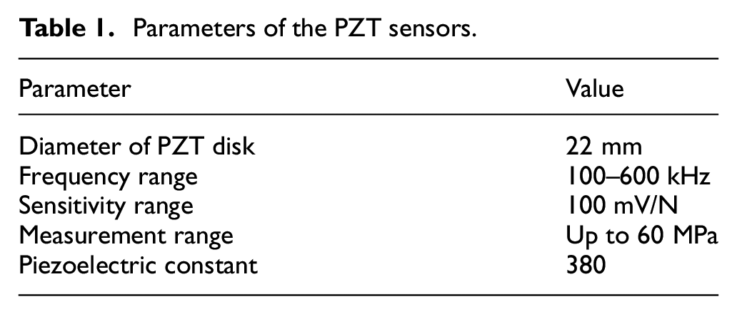
An AE-based monitoring system was previously developed by the authors^19,21,49 for online rail turnout crack detection. The system includes a set of encapsulated piezoelectric (PZT) sensors, a four-channel National Instrument 9223 Pickering card (1 MHz sampling rate) that is able to collect data from four sensors simultaneously, and a computer for data storage. Specific parameters of the PZT sensors are displayed in Table 1. The schematic of the system can be seen in Figure 2, and the collected data were eventually stored in the database located in the control room near the rail turnout area for further analysis.

Table 1.

Parameters of the PZT sensors.

Parameter	Value
Diameter of PZT disk	22 mm
Frequency range	100–600 kHz
Sensitivity range	100 mV/N
Measurement range	Up to 60 MPa
Piezoelectric constant	380

Figure 2.

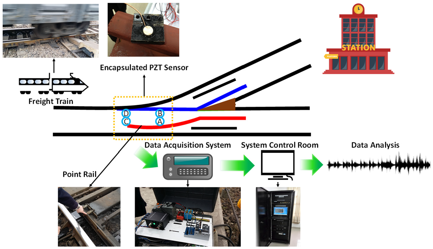
The AE-based monitoring system for rail turnout crack detection.

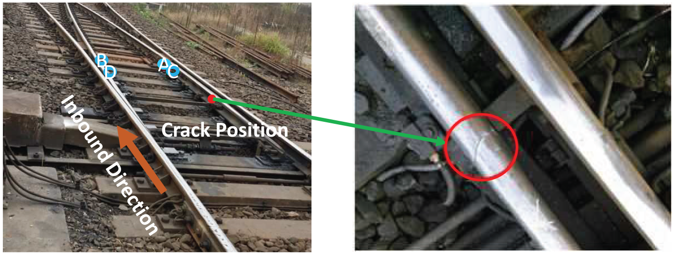
The system was initially deployed at a rail turnout area of an in-service freight line near a freight station in mainland China. According to reports from the partner rail operators, the point rails on the two sides are most vulnerable to damages due to the irregular rail profile, frequent switching, and constant impacts from freight trains. In recognition of this, four PZT sensors were mounted at the rail foot of the point rails on the inbound route (two sensors numbered as A and C on the left rail and two sensors numbered as B and D on the right rail), as shown in Figure 3, covering a 10 m monitoring area. When any train passes through the monitored rail turnout area, the data acquisition component would be triggered and start taking measurements for 8 s adequate to record full responses induced by a common eight-cargo freight train that normally passes at a speed of around 20–40 km/h within the station’s nearby area. It has been investigated in the pilot study that the acoustic burst frequency caused by rail crack expansion mostly lies in a range from ultrasonic frequency (20 kHz) to 140 kHz,¹⁹ and the sampling rate is set to be 600 kHz to fully capture the frequency range of interest. The monitoring system was in-service for three years taking acoustic recordings intermittently. Despite the large number of data points (4.8 million) in every 8 s recording, it should be noted that each recording is treated as one sample for DL, and thus the number of samples is relatively small due to the trigger-measure mechanism. Passing locomotives are either multiple-cargo freight trains (in normal operation hours) or one-cargo train (in rail shunting period). Typical recordings triggered by one-cargo train and multiple-cargo train is shown in Figure 4. It can be observed from Figure 4 that in one single recording, each passing cargo induced significant and relevant vibrations and noises, manifested as acoustic peaks with amplitude ranging from 0.4 to 15 V. While according to our pilot lab testing, the acoustic peaks excited by crack expansion are often relatively small, obscured by wheel–rail interaction-induced waveforms in the time domain.

Figure 3.

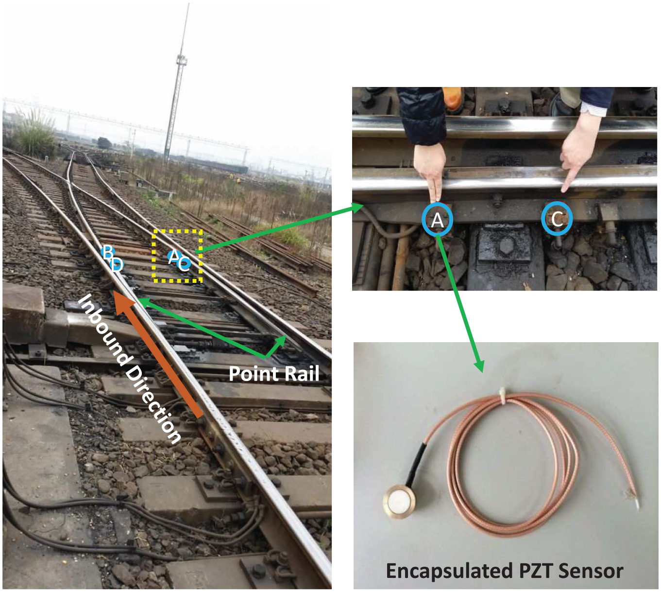
Sensor implementation position at rail turnout area.

Figure 4.

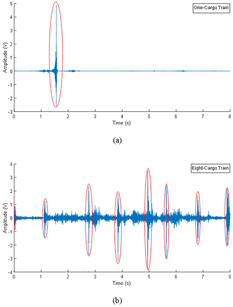
AE recordings triggered by (a) one-cargo train and (b) eight-cargo train.

Data description

A significant crack at the railhead of the right point rail corresponding to the inbound direction was spotted in mid-November 2014 by manual detection (Figure 5). The crack occurred 2 m away from sensor C but was missed by the monitoring system. The point rail was confirmed by our partner rail operator to be intact before early October. Therefore, the data recorded from September to November 2014 was used in this study covering a continuous deterioration period of the point rail from intact to cracked. When the rail was intact, no AE induced by crack expansion can be measured. When microcrack had initialized, it would increase in size every time a freight train passed by and generated AE burst hidden in the strong background noises. The pattern of the burst, in turn, reflected its current condition. This is the basic assumption of monitoring turnout crack based on AE techniques. To reveal the progressing crack, we divided the crack growing period into several stages. The dataset is divided into four stages: Stage I-intact, Stage II, Stage III, and Stage IV-significantly cracked. This four-stage option is a balance between sufficiency and necessity in proving the concept. According to the mechanism of fatigue growth, a typical rail crack growing under heavy freight loading condition where the crack growth rate is increasing with respect to time,^50–54 the period of each stage should be decreasing, as schematically shown in Figure 6. Therefore, 1-month AE recordings (3524 samples) were used as Stage I data, 2-week recordings as Stage II data (946 samples), 1-week recordings (482 samples) as Stage III data, and 4-day recordings (584 samples) as Stage IV data. Time gaps are reserved between neighboring stages of data selection to guarantee distinction, and more recordings were chosen in Stage IV for better training performance. Figure 7 demonstrates the AE recordings of rail under four stages and the PSDs of these signals are shown in Figure 8, focusing on the frequency interval between 20 and 140 kHz. It should be noted that Figures 7 and 8 are just samples grabbed from the dataset for demonstration and we do not expect to directly observe the pattern that can reflect the crack progress in either time domain or frequency domain.

Figure 5.

The rail with significant crack.

Figure 6.

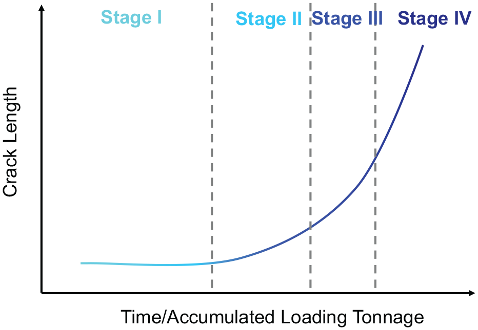
Progress of rail crack and stage classification.

Figure 7.

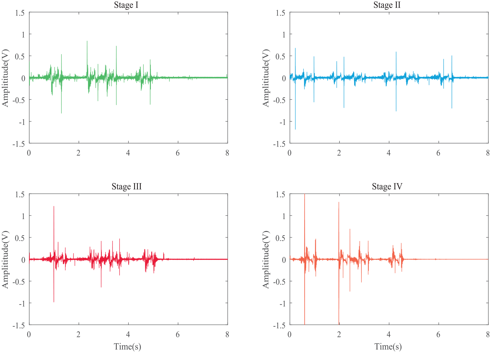
AE recordings of rail under four stages subject to impact of eight-cargo trains.

Figure 8.

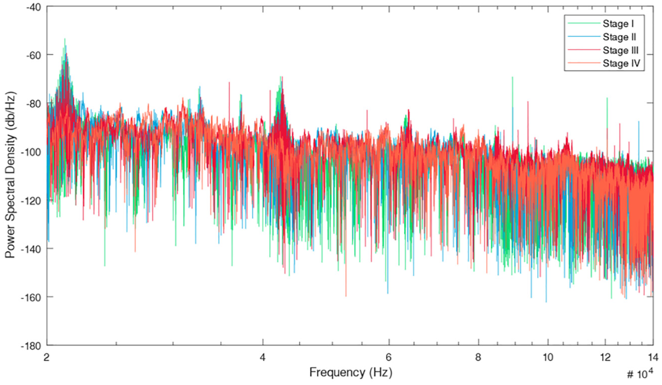
Power spectral density of AE recordings of four stages.

Methodologies

The flowchart of the proposed approach is illustrated in Figure 9. First of all, the raw AE signals were represented in the time–frequency domain. An audio source domain that is closely related to our target domain as well as the model N_A pre-trained on it with a sophisticated source task (527 categories) was selected. Subsequently, the low-level layers of N_A were transferred to our model and the parameters were frozen. Then, the high-level layers were further developed and trained using the AE monitoring data in the target domain. When new AE monitoring data arrives, it first goes through the frozen layers and then the trainable layers to evaluate the stages of rail conditions. MMD was calculated between the output of audio source data and AE monitoring data to quantify the relevance. The proposed approach is demonstrated in detail through the following subsections.

Figure 9.

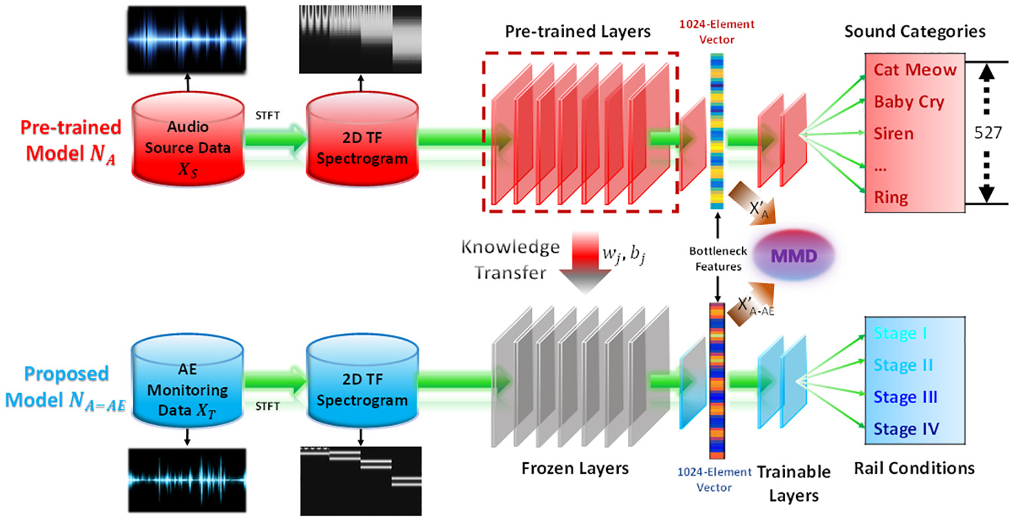
Flowchart of the proposed approach.

Time–frequency representation

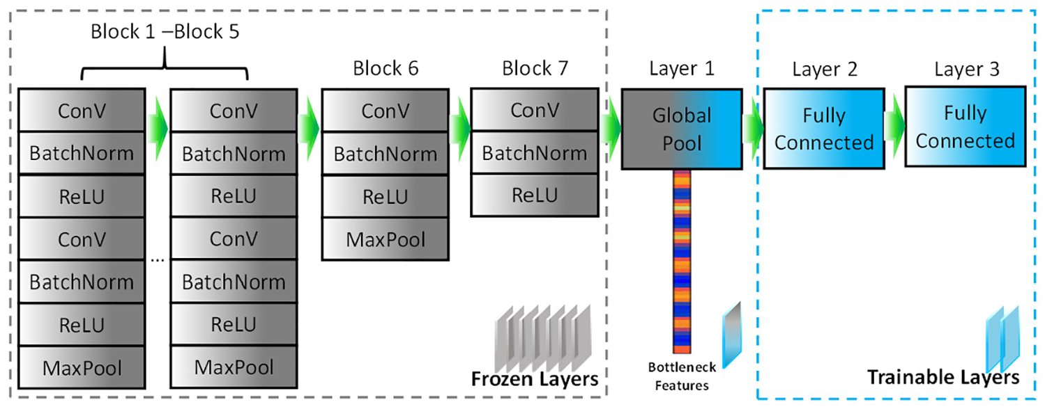
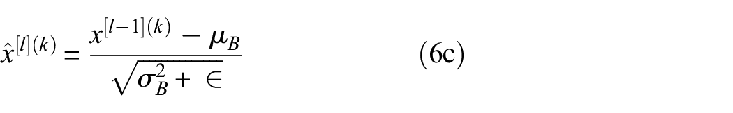
Before the construction of the model, it is necessary to conduct pre-processing on the AE monitoring data. For acoustic waveforms, time–frequency spectrograms that contain rich information in both time and frequency domains are often used for further analysis.⁵⁵ Specifically, we conducted short-term Fourier transform (STFT) to the AE signals and obtained their spectrograms as

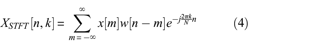
X_{STFT} [n, k] = \sum_{m = - \infty}^{\infty} x [m] w [n - m] e^{- j \frac{2 π k}{N} n}

(4)

where w is a window function and $x [m] w [n - m]$ is a short-time section of signal $x [m]$ at time n.

One AE signal was divided into 4688 segments using a Hann window with a size of 2048 (assuming that the signal within 3.41 ms is stationary) and overlap of 1024. The PSD was calculated for each segment to generate a spectrogram.

According to our previous study,²¹ the PSD values of signals containing damage information reaches 90 to 140 kHz among all the frequency bands. To ensure the information in the ultrasonic level is fully made use of, we adopted the spectrum under a frequency range between 20 and 140 kHz. The PSD values were then combined into 128 frequency bins. Therefore, the size of the spectrogram is 128 × 4688. Figure 10(a) and (b) illustrate one AE signal and its spectrogram. It should be noted that the spectrum is displayed in Gray Plot because we were using the direct PSD values rather than the red, green and blue (RGB) decompositions as input to our model, and this will be further explained in the section “Construction of A-AE TL model.”

Figure 10.

(a) AE recording, (b) AE spectrogram, (c) audio recording, and (d) audio spectrogram.

Selection of source domain

As illustrated at the beginning of this article on source domain selection, we would like the source data to be as close as possible to the target data. Basically, each AE burst (subject to impact, noise, and crack expansion) is considered as an audio event, and a segment of online audio recording also contains one or multiple audio events. This motivates us to use an online audio database as the source domain aiming at a better performance. The intuitive thinking is validated through MMD and will be elaborated in the section “MMD comparison.”

There are multiple online open-access audio database options, among which AudioSet dataset,⁵⁶ a large-scale dataset of manually annotated audio events, is considered to be a good source dataset. The dataset consists of around 2.1 million 10 s audio recordings for 527 sound events,⁵⁷ each of which at least contains 59 samples. The advantages of this dataset are two-fold. First, it has a close domain relation to our dataset, which contains different kinds of sound events. One recording is shown in Figure 10(c). The waveform is found similar to ours. More importantly, it has a large vocabulary (527 kinds of sound events), which makes the model it nurtures able to extract robust enough features for generic tasks. These sound events include sounds of things (engine, bell, alarm, mechanisms, etc.) and source-ambiguous sounds (generic impact sounds, surface contact, deformable shell, etc.) among others. Another typical audio dataset, in comparison, ESC-50 dataset⁵⁸ is too small because it consists a total of only 2000 recordings of 50 sound events.

It is found that CNN-like structures work well on audio classification by analyzing popular CNN architectures such as VGG,⁴⁰ ResNet⁵⁹ for large-scale sound event classification on web videos.⁶⁰ The import properties of CNNs are local connectivity and parameter sharing in convolutional layers, which means that the filters can extract local features even when the frequency range is different between spectrograms of source data and target data. Thus, a CNN trained on AudioSet,⁶¹ dominated as N_A, is leveraged in our study.

N_A can be divided into two parts. The first part is a feature extractor, which intakes the spectrogram of an audio recording, such as Figure 10(d), and outputs generic features, based on which, the second part, a classifier, can identify 527 sound events occurred within 10 s. Due to the underneath relation between audio data and AE data, the feature extractor is very likely to be applicable for AE data, and thus be transferred as the frozen layers in our model. The construction of our model is detailed in the section “Construction of A-AE TL model.”

Construction of A-AE TL model

The developed model is named N_A-AE, which means that it is a “Network trained on AE data with knowledge transfer from Audio.” N_A-AE intakes a spectrogram directly, and, like a typical CNN model, transforms this input into a more and more abstract and composite representation layer by layer, and finally predicts the rail condition. This process is forward propagation.

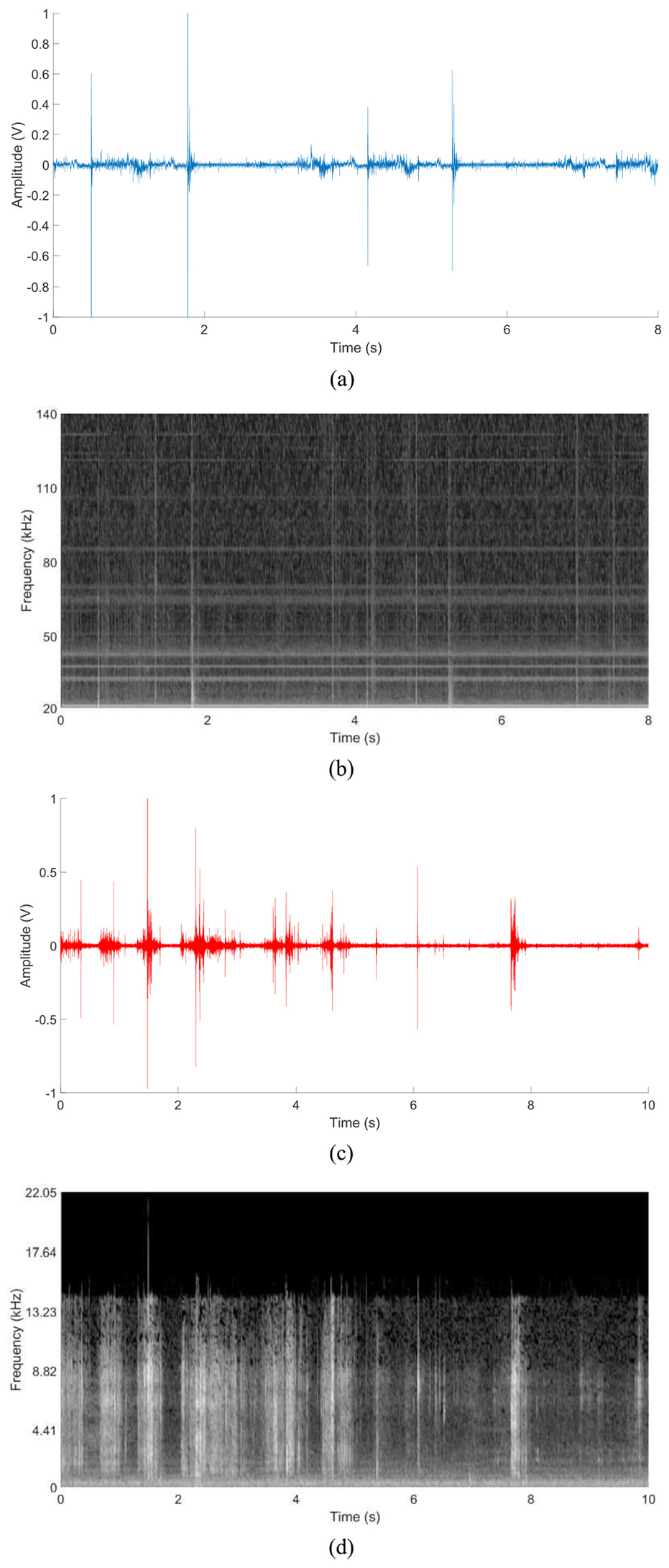
Figure 11 shows the architecture of N_A-AE, which consists of seven blocks (each block with multiple layers) for segment-level feature extraction, a fusion layer for the integration of extracted features and two layers for mapping the bottleneck features to the prediction of condition. The output representation x of each block (layer) is summarized in Table 2. The three dimensions donate [depth, height, width], that is., [feature, time, frequency]. The operations conducted in a Block for an input volume, including Convolution (Conv), Batch Normalization (BatchNorm), Restricted Linear Unit (ReLU), Maximum Pooling (MaxPool), Global Pooling (GlobalPool), and Fully Connected (FC) feedforward, will be introduced in the sub-subsections.

Figure 11.

Architecture of the proposed model.

Table 2.

Representations generated by each block (layer).

Block/Layer	Operations	Conv filters	Size of output representation
Input		None	1 × 4688 × 128
Block 1	(Conv→BatchNorm→ReLU) × 2→MaxPool	16 3 × 3 filters	16 × 2344 × 64
Block 2	(Conv→BatchNorm→ReLU) × 2→MaxPool	32 3 × 3 filters	32 × 1172 × 32
Block 3	(Conv→BatchNorm→ReLU) × 2→MaxPool	64 3 × 3 filters	64 × 586 × 16
Block 4	(Conv→BatchNorm→ReLU) × 2→MaxPool	128 3 × 3 filters	128 × 293 × 8
Block 5	(Conv→BatchNorm→ReLU) × 2→MaxPool	256 3 × 3 filters	256 × 146 × 4
Block 6	(Conv→BatchNorm→ReLU) × 1→MaxPool	512 3 × 3 filters	512 × 73 × 2
Block 7	(Conv→BatchNorm→ReLU) × 1	1024 2 × 2 filters	1024 × 72 × 1
Layer 1	GlobalPool	None	1024 × 1 (bottleneck features)
Layer 2	FC→ReLU	None	64 × 1
Layer 3	FC→Softmax	None	4 × 1

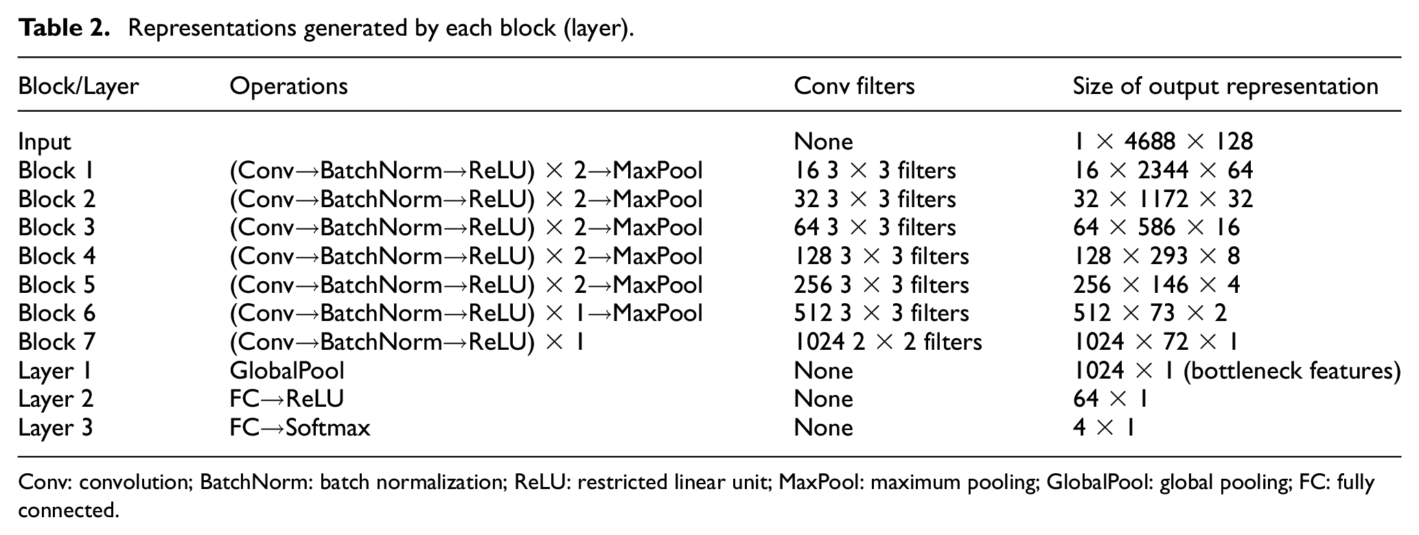
Conv: convolution; BatchNorm: batch normalization; ReLU: restricted linear unit; MaxPool: maximum pooling; GlobalPool: global pooling; FC: fully connected.

Frozen layers

Block 1 to Block 5 consists of two Conv layers (with BatchNorm) followed by a MaxPool. Block 6 consists of one Conv layer, followed by a MaxPool layer. ReLU is used in all cases. For convolutional layers in all six blocks, $3 \times 3$ filters are used. Stride and padding are fixed to 1. The numbers of filters used in convolutional layer(s) from Block 1 to Block 6 are 16, 32, 64, 128, 256, 512, respectively. MaxPool is done over a 2 × 2 window, with a stride of 2 × 2. In Block 7, 1024 filters of size 2 × 2 are used with a stride of 1. The parameters, including the $w^{[l]}$ , $b^{[l]}$ , $γ^{[l]}$ , and $β^{[l]}$ , are transferred from the pre-trained model and frozen N_A. The input volume (spectrogram of AE signal) is denoted as $x^{[0]}$ with size of $n_{D} \times n_{H} \times n_{W}$ .

Conv layer consisting of a set of learnable filters is used to extract local feature maps. Each filter is spatially small but extends through the full depth of the input volume. During the forward propagation, each filter slides across the width and height of the input volume and compute dot products between the weights of the filter and the entries of the receptive field (the region that the filter is looking at). This convolution can be considered as feature extraction and finally produces a two-dimensional (2D) feature map containing the activations of that filter at every spatial position. The set of filters generates a number of feature maps. In summary, in a Conv layer numbered $[l]$ with $n_{D}^{[l]}$ learnable filters, the jth filter generates a feature map $x_{j}^{[l]}$ from an input volume $x^{[l - 1]}$

x_{j}^{[l]} = w_{j}^{[l]} * x^{[l - 1]} + b_{j}^{[l]}

(5)

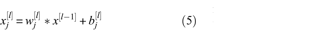
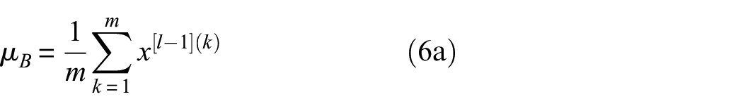
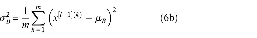
where * represents the convolutional operator; $w_{j}^{[l]}$ and $b_{j}^{[l]}$ are the weight volume and bias volume of the jth filter, respectively. The stacked $n_{D}^{[l]}$ feature maps give the activations $x^{[l]}$ .

BatchNorm⁶² is used to mitigate this internal covariate shift issue and thus accelerate the convergence of the training. During training, in the intermediate layers, the distribution of activations from the previous layer is constantly changing, which slows down the training process because each layer must learn to adapt themselves to a new distribution at every training step. Given the activations from the previous layer numbered $[l - 1]$ over a mini-batch: $B : {x^{[l - 1] (1)}, \dots, x^{[l - 1] (m)}}$ , the BatchNorm layer, with two learnable parameters $γ^{[l]}$ and $β^{[l]}$ , conduct the following operations to normalize, scale, and shift the activations

μ_{B} = \frac{1}{m} \sum_{k = 1}^{m} x^{[l - 1] (k)}

(6a)

σ_{B}^{2} = \frac{1}{m} \sum_{k = 1}^{m} {(x^{[l - 1] (k)} - μ_{B})}^{2}

(6b)

{\hat{x}}^{[l] (k)} = \frac{x^{[l - 1] (k)} - μ_{B}}{\sqrt{σ_{B}^{2} + \in}}

(6c)

BatchNor m_{γ, β} (x^{[l - 1] (k)}) \equiv x^{[l] (k)} = γ^{[l]} {\hat{x}}^{[l] (k)} + β^{[l]}

(6d)

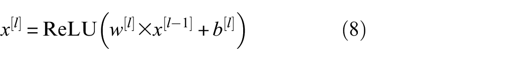
The feature maps are passed through a nonlinear activation function, ReLU,⁶³ which is elementwise and remains the size of the volume

ReLU (x) = \max (x, 0)

(7)

Pooling layer is used to shrink the volume of representation and reduce the number of parameters in the next layer to train. MaxPool is commonly used, which takes the max over four numbers in every 2 × 2 region of the input volume. The layer can maintain the depth dimension $n_{D}$ and disregard 75% of the previous activations by using MaxPool operation with a stride of 2 on every depth slice.

Segment integration and trainable layers

As shown in Table 2, the frozen layers intake the spectrogram of [1 × 4688 × 128] and produce the plate-like representation (after Block 7) of [1024 × 72 × 1] (order: feature, time, frequency). These segment-level features retain the information on the time axis. To integrate the segment-level representation into recording-level representation, GlobalPool is used. Basically, it takes the largest value along the time axis and generates 1024 features for the whole recording. This process enables our approach to flexibly handle AE recordings with different lengths. The 1024 features can be considered as a highly condensed version of the whole recording and they are called bottleneck features because they exactly locate in the bottleneck position before the classifier.

A multi-layer perceptron (MLP) consisting of several fully connected layers is used as a classifier after the global pooling to nonlinearly map the bottleneck features to the evaluation of rail condition corresponding to the AE data. For an input volume $x^{[l - 1]}$ , the output of one layer is

x^{[l]} = ReLU (w^{[l]} \times x^{[l - 1]} + b^{[l]})

(8)

The final score for four classes is given by

\hat{y} = σ (w^{[L]} \times x^{[L - 1]} + b^{[L]})

(9)

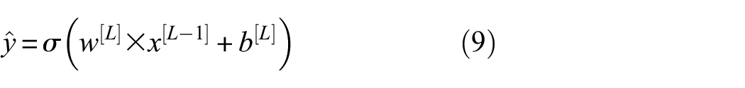
where $σ$ is the Softmax function.

The hyper-parameters of MLP, including the number of layers and the size of each hidden layer, are selected using fivefold cross-validation.⁶⁴ Specifically, the training dataset is randomly partitioned into five equal-sized sub-datasets. For each sub-dataset, the remaining four sub-datasets are used for training. For one hyper-parameter setting, the evaluation is conducted for five sub-datasets and the average cost (cross entropy) reflects the performance of current setting. Finally, a two-layer (Layer 2 and Layer 3) perceptron with a hidden layer size of 64 is selected due to its lowest cost.

In the process of training, the model typically takes a mini-batch with m samples and compares the final predictions to the ground truth. The cost (error) is back-propagated to update the parameters of each layer and thus gradually reduced by traversing all mini-batches within the training set for many epochs. The cost function is cross entropy

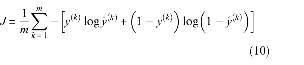
J = \frac{1}{m} \sum_{k = 1}^{m} - [y^{(k)} \log {\hat{y}}^{(k)} + (1 - y^{(k)}) \log (1 - {\hat{y}}^{(k)})]

(10)

where for the kth sample in the mini-batch, $y_{k}$ is a one-hot vector that indicates the true class, such as ${[0100]}^{T}$ ; and ${\hat{y}}_{k}$ is a vector that contains the probability of each class.

The training set contains 2880 samples, taking around 55% of the data. Of them, 320 samples are used as a validation set during the training. Based on these samples, the N_A-AE was trained in the Pytorch framework. As described in the section “Construction of A-AE TL model”, the parameters of Block 1 to Block 7 were frozen and those in Layer 9 to Layer 10 were tuned. Dropout⁶⁵ with a rate of 0.5 was used in Layer 2 to prevent overfitting. The cost function was cross entropy. The optimization was conducted using an Adam optimizer⁶⁶ with a learning rate of 0.0001. The training will be conducted until the cost function on the validation set converges. The minibatch size was set as 32 so there are 90 mini-batches in the training set.

After learning from the training data, the model represents an inferred function, which can be used to map new samples. The performance of the N_A-AE is investigated in the section “Performance comparison” in comparison with other baselines.

Baseline methods

VGGNet⁴⁰ is a highly successful model in the field of computer vision (CV) for image classification, which has been pre-trained on ImageNet.⁴¹ Its ability to extract robust features from normally taken photos have been proved. On this basis, one baseline network, named N_I-AE is developed. The formulation of N_I-AE basically follows the idea of N_A-AE. VGGNet consists of five convolutional blocks (Conv1–Conv5) and three fully connected layers (FC0–FC2). The convolutional blocks and FC0 are frozen and copied to N_I-AE followed by an MLP with two FC layers. The whole N_I-AE is then retrained on AE data.

The process is illustrated in Figure 12. The source model N_I requires an input of a three-channel image with a size of 224 × 224. Since the spectrogram itself is typically wider and has only one channel, it has to be cropped or resized and then either stacked three times or decomposed into RGB compositions to pretend a three-channel image to fit the requirement of VGGNet. The matrix stacking or RGB decomposing behavior in N_I-AE may be brutal and does not increase any information compared to the straightforward data intaking way in N_A-AE as shown in Figure 9. In addition, it should be noted that the source domain seems to be far away from the target domain in nature, especially in comparison with the case in Figure 10. The MMD results measuring their discrepancy are also shown in the section “MMD comparison.”

Figure 12.

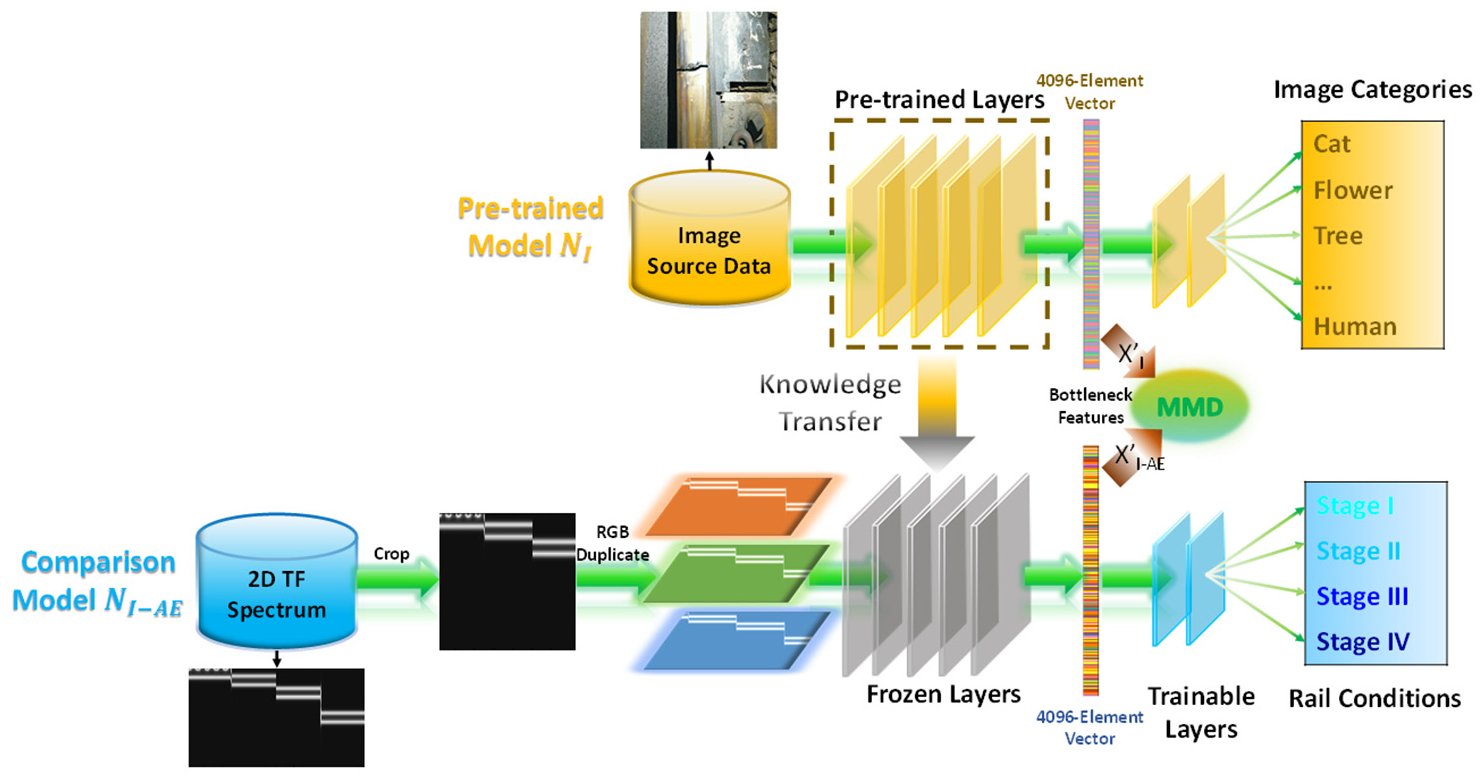
Flowchart of TL model N_I-AE.

Another baseline network for comparison is a conventional CNN model that is trained from scratch, noted as N_AE. The parameters in the frozen layers (referred to Figure 11) are unfrozen and randomly initialized rather than transferred from N_A, and the whole model is trained on AE data.

To make the comparison more comprehensive, another method without the involvement of DL is also used. One MLP is developed so as to learn and evaluate the rail condition based on the PSD of the AE waveforms. It should be noted that an MLP is a classic feedforward neural network with an input layer, an output layer, and several trainable weight layers. This method is named “PSD + MLP.”

MMD calculation

Calculating MMD between distributions of input spectrograms is certainly possible, but normally we would like to know the discrepancy of inner essence (e.g. acoustic-specific) between datasets, while an original spectrogram may contain a lot of unwanted information that would dilute the MMD outcomes. Therefore, in practice, many studies tend to measure the domain discrepancy between distributions of bottleneck features rather than those of the original data (spectrograms),^44,45 and this is what we use in this study.

General MMD calculation is demonstrated in the section “TL and MMD.” For the case of this study, given data $X_{A}$ (audio data from AudioSet) from the source domain $D_{A}$ and $X_{AE}$ (AE monitoring data) from the target domain $D_{AE}$ , and STFT were conducted to generate 2D time–frequency spectrograms. The low-level layers of the well-trained model N_A construct a feature extractor, which can intake the spectrogram of audio data and generate bottleneck features $X'_{A}$ . Similarly, bottleneck features $X'_{A - AE}$ corresponding to $X_{AE}$ can be obtained, as shown in Figure 9. MMD between $D_{A}$ and $D_{AE}$ is calculated based on the bottleneck features

\begin{matrix} MM D_{A, AE} = MMD [K, {X'}_{A}, {X'}_{A - AE}] \\ = {[\frac{1}{m} \sum_{i, j = 1}^{m} k ({x'}_{A, i}, {x'}_{A, j}) + \frac{1}{n} \sum_{i, j = 1}^{n} k ({x'}_{A - AE, i}, {x'}_{A - AE, j}) - \frac{1}{mn} \sum_{i, j = 1}^{mn} k ({x'}_{A, i}, {x'}_{A - AE, j})]}^{\frac{1}{2}} \end{matrix}

(11)

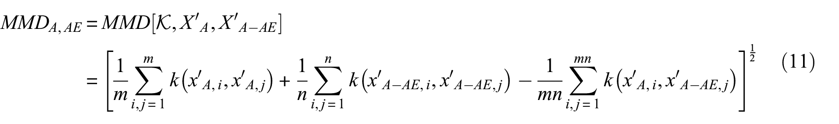
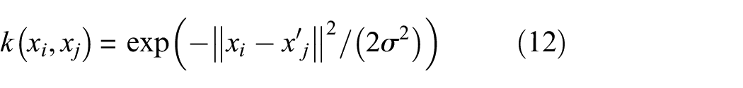
In this study, three kinds of kernels were used including linear kernel $k (x_{i}, x_{j}) = x_{i}, x_{j}$ , polynomial kernel $k (x_{i}, x_{j}) = x_{i}, {x_{j}}^{k}$ (where $x_{i}, {x_{j}}^{k}$ denotes the kth power of the inner product between $x_{i}$ and $x_{j}$ ), and radial basis function (RBF) kernel

k (x_{i}, x_{j}) = \exp (- {‖ x_{i} - {x'}_{j} ‖}^{2} / (2 σ^{2}))

(12)

where $σ$ is the kernel width parameter.

For TL model N_I-AE, MMD between the source domain $D_{I}$ (ImageNet) and $D_{AE}$ was calculated through the same procedures. MMD results are shown in the section “MMD comparison.”

Results and discussion

Performance comparison

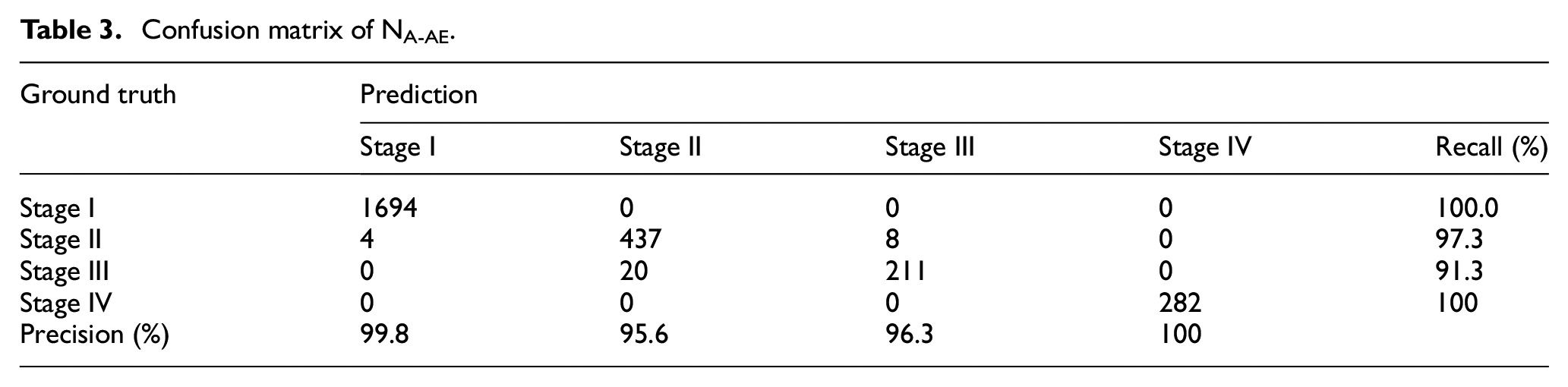
Model training, validating, and testing process was conducted on a workstation with an Intel(R) Core(TM) i7-7700HQ 2.8 GHz processor, 12 GB RAM, and an Nvidia GTX1070 Graphic Card. The well-trained N_A-AE was used to infer the unseen data (size = 2656) in the testing set. The inferred rail condition is the category with the highest probability. Table 3 shows the confusion matrix. The recall and precision for each condition are also calculated. It is found that the model can well classify the AE recordings of each condition. The high precision of Stage I means that false alarm is very rare. On the contrary, the high recall of Stage II and Stage III means that the development of crack can be identified as early as possible, although few Stage III recordings are mistaken as Stage II.

Table 3.

Confusion matrix of N_A-AE.

Ground truth	Prediction
Ground truth	Stage I	Stage II	Stage III	Stage IV	Recall (%)
Stage I	1694	0	0	0	100.0
Stage II	4	437	8	0	97.3
Stage III	0	20	211	0	91.3
Stage IV	0	0	0	282	100
Precision (%)	99.8	95.6	96.3	100

The F1 score for each class i is shown in the first column of Table 4, which is calculated by

F 1_{i} = 2 (\frac{recal l_{i} \times precisio n_{i}}{recal l_{i} + precisio n_{i}})

(13)

Table 4.

Comparisons between N_A-AE and baseline methods in terms of F1.

	N_A-AE (%)	N_I-AE (%)	N_AE (%)	PSD + MLP (%)
Stage I	99.9	98.9	99.7	99.9
Stage II	96.5	85.5	86.0	79.6
Stage III	93.8	60.2	64.5	52.9
Stage IV	100.0	100.0	99.8	100.0
Average	97.5	86.1	87.5	83.1

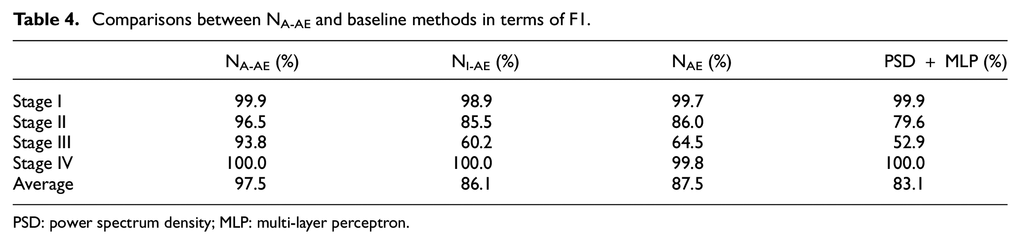
PSD: power spectrum density; MLP: multi-layer perceptron.

The mean of F1 for four classes, called macro-F1 was used as a summarized metric. Overall, the macro-F1 of N_A-AE is 97.5%. In comparison, the macro-F1 of N_I-AE and N_AE is 86.1% and 87.5%, respectively. This indicates that the knowledge transferred from ImageNet has no benefits or even negative influences on the evaluation performance. Details for each stage are shown in Table 4. Although all three models can well identify the Stage IV, that is., the existence of critical crack, the F1 score of Stage III in N_I-AE and N_AE recordings is only 60.2% and 64.5%, respectively, which means these two models can hardly distinguish the middle transition stages of rail conditions, while N_A-AE can classify Stage II and Stage III with satisfactory performance.

It should be noted that the method without the involvement of DL does not perform well in terms of F1 score, which should be blamed on the non-optimal features. After all, the PSD throws out the time information.

It is worth mentioning that it is also possible to unfreeze and fine-tune more high-level layers as an attempt to elevate the performance of N_I-AE for a more comprehensive comparison with N_A-AE. For N_I-AE, three configurations of fine-tuning are investigated: (1) Tuning F0; (2) Tuning F0 and Conv5; and (3) Tuning F0, Conv5, and Conv4. The corresponding models are named N_I-AE-1, N_I-AE-2, and N_I-AE-3, respectively. The average macro-F1 scores under different fine-tuning configurations are plotted in Figure 13. It can be seen from Figure 13 that despite the increasing F1 score under more layers unfrozen and profound fine-tuning, N_A-AE without any fine-tuning process still outperforms N_I-AE for all configurations. Moreover, unfreezing more layers would definitely increase the labor of training and lower the status and function of transferred knowledge in TL. Under the extreme state when all low-level layers are unfrozen, the TL model degenerates back into a conventional CNN model.

Figure 13.

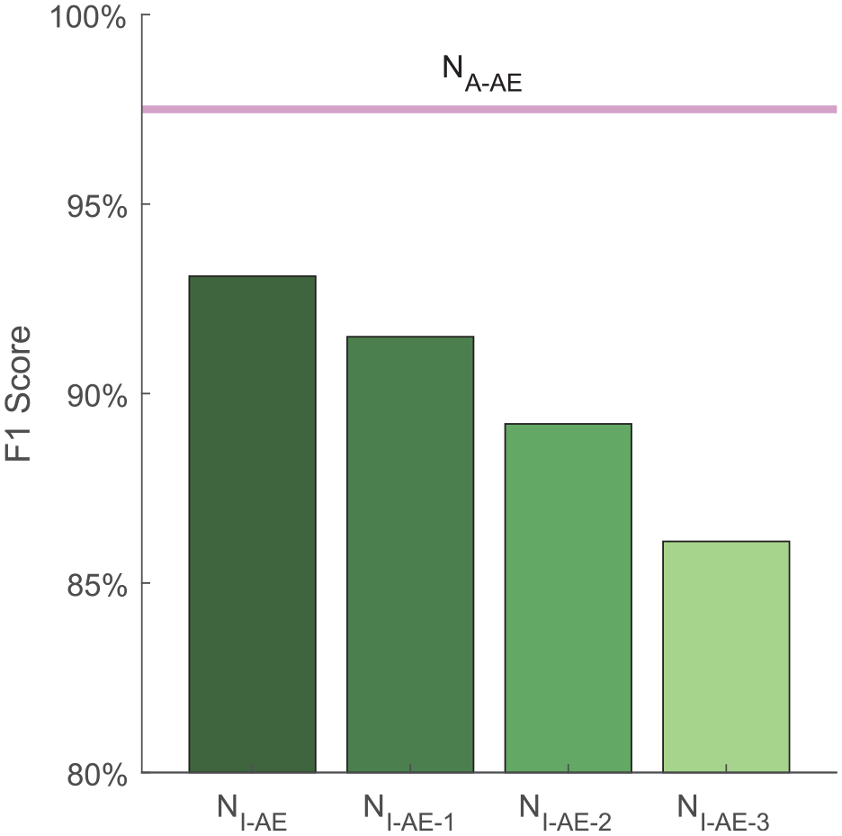
F1 score of N_I-AE after fine-tuning.

MMD comparison

Following the calculation procedures in the section “MMD calculation,” the MMD between $X'_{I}$ and $X'_{I - AE}$ (denoted as MMD_I,AE), as well as $X'_{A}$ and $X'_{A - AE}$ (denoted as MMD_A,AE) can be obtained. For N_I-AE, it should be noted that $X'_{I}$ consists of the bottleneck features extracted by N_I from 5536 images randomly selected from ImageNet. Since $X'_{A}$ and $X'_{A - AE}$ are 1024-element vectors and $X'_{I}$ and $X'_{I - AE}$ are 4096-element vectors, MMD is calculated between the 1024-dimensional or 4096-dimensional joint distributions. Certainly, such high-dimensional distributions cannot be directly plotted as figures, but we can plot distributions of elements in the bottleneck features separately to catch a glimpse of the whole view and necessity of using MMD here. Figure 14(a) shows distribution comparisons of some elements in $X'_{A}$ and $X'_{A - AE}$ , and Figure 14(b) shows distribution comparisons of some elements in $X'_{I}$ and $X'_{I - AE}$ .

Figure 14.

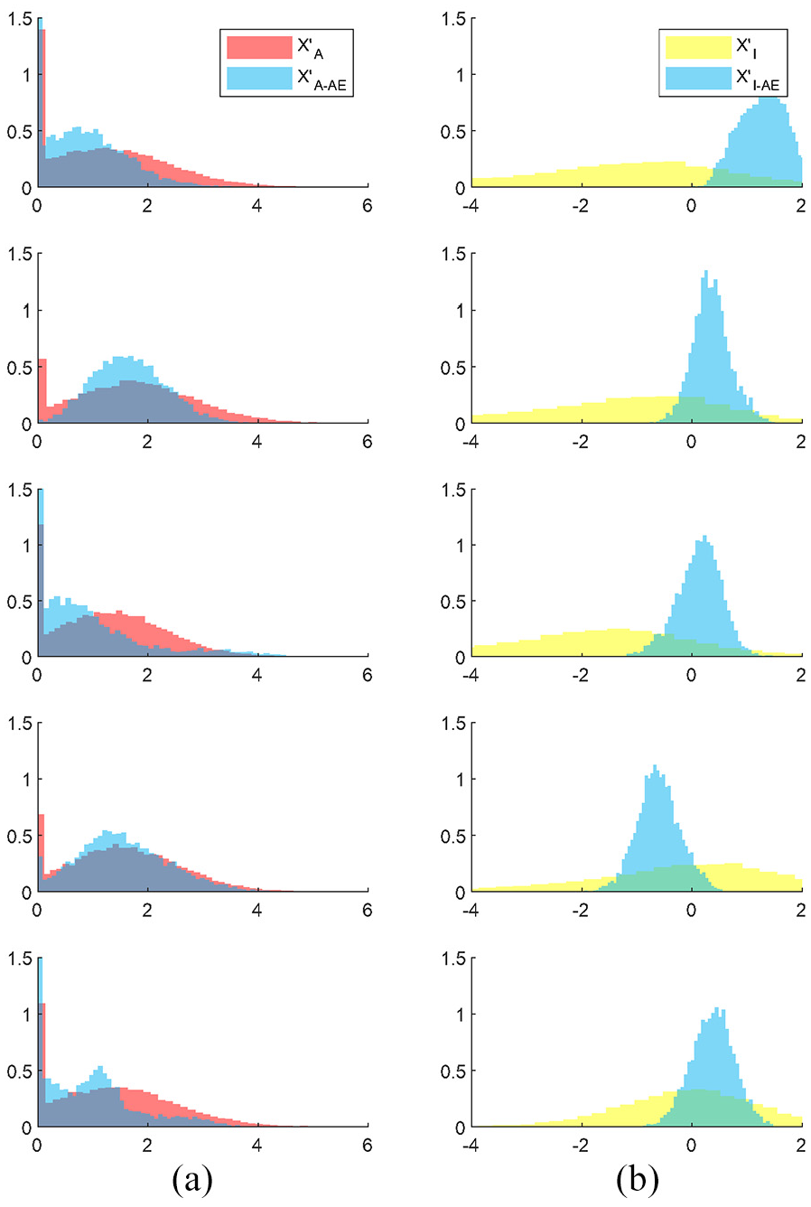
Distribution comparison between elements in (a) $X'_{A}$ and $X'_{A - AE}$ and (b) $X'_{I}$ and $X'_{I - AE}$ .

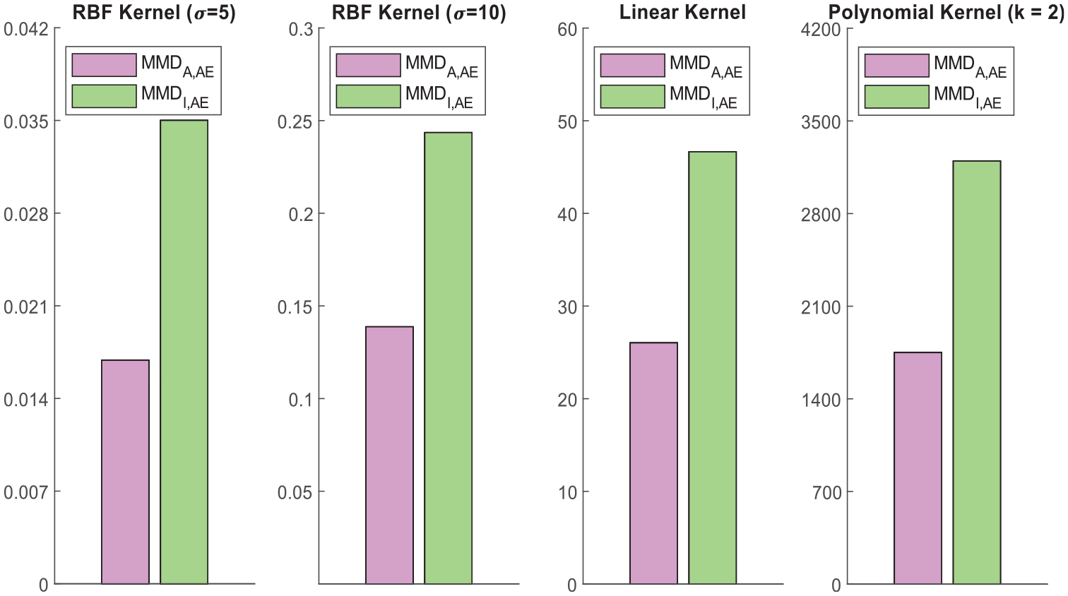
To guarantee the MMD comparison is sufficiently general and convincing, four kernel functions under three types (RBF, Linear, and Polynomial) were used in this study. As introduced in the section “TL and MMD,” each kernel represents one kind of mapping to RKHS. The kernel width parameter $σ$ of RBF kernel is chosen to be 5 and 10, respectively, and the degree k of polynomial kernel is 2. The comparison is shown in Figure 15. Note that the vertical scales are different due to the different kernels. It can be observed that under four kernel functions, the values of MMD_A,AE are all significantly smaller than MMD_I,AE values. This result coincides with our intuitive sense and is in alignment with the performance of the corresponding models in Table 4 and Figure 13.

Figure 15.

Domain discrepancy between AE and Audio and that between AE and Image.

Visualization of bottleneck features

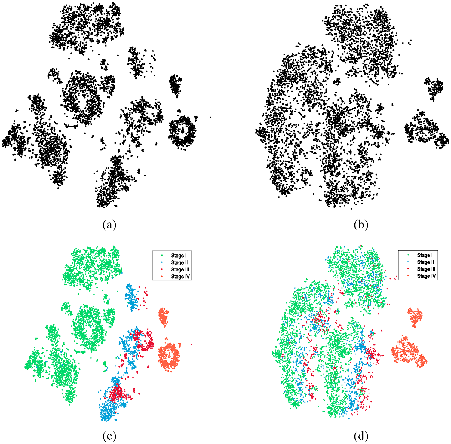
There are 5536 AE recordings totally. When they are fed to N_A-AE or N_I-AE, 5536 sets of bottleneck features can be generated, denoted as $X'_{A - AE}$ or $X'_{I - AE}$ , respectively. To obtain a straight view of the bottleneck features, t-distributed Stochastic Neighbor Embedding (t-SNE)⁶⁷ is used to visualize the bottleneck features $X'_{A - AE}$ and $X'_{I - AE}$ generated by N_A-AE and N_I-AE. The t-SNE is a nonlinear dimensionality reduction technique for embedding high-dimensional data for visualization in a low-dimensional space of two or three dimensions. It should be noted that the process of feature extraction and dimension reduction is without any involvement of supervised training.

The results are illustrated in Figure 16. Each point in the figure represents the embedding features of an AE record. In Figure 16(a), bottleneck features from N_A-AE seem to exhibit several clusters; while in Figure 16(b), features from N_I-AE seem to mix up. When they are colored according to the type, it can be found that features from the same rail condition tend to cluster and there exists obvious borders between clusters in Figure 16(c). It should be noted that there is also a subtle trend of the points that reflect the progress of cracks. This result shows that the frozen layers of N_A-AE are able to extract meaningful features for further classification. In comparison, the features of Stage I to class Stage III from N_I-AE are mixed up in Figure 16(d). This indicates that the useful information is corrupted by a not-so-relevant model and to some degree lead to a performance decay.

Figure 16.

Visualization of bottleneck features $X'_{A - AE}$ and $X'_{I - AE}$ : (a) Features from N_A-AE, (b) features from N_I-AE, (c) colored features from N_A-AE, and (d) colored features from N_I-AE.

After labels were annotated in Figure 16(c), when we investigate 16(a) again it is found that although Stage II and Stage III cannot be clearly separated in the figure, the clustering phenomena of features from Stage I (intact) and Stage IV (critically cracked) implies the possibility to evaluate the rail condition in an unsupervised way.

Computation time comparison

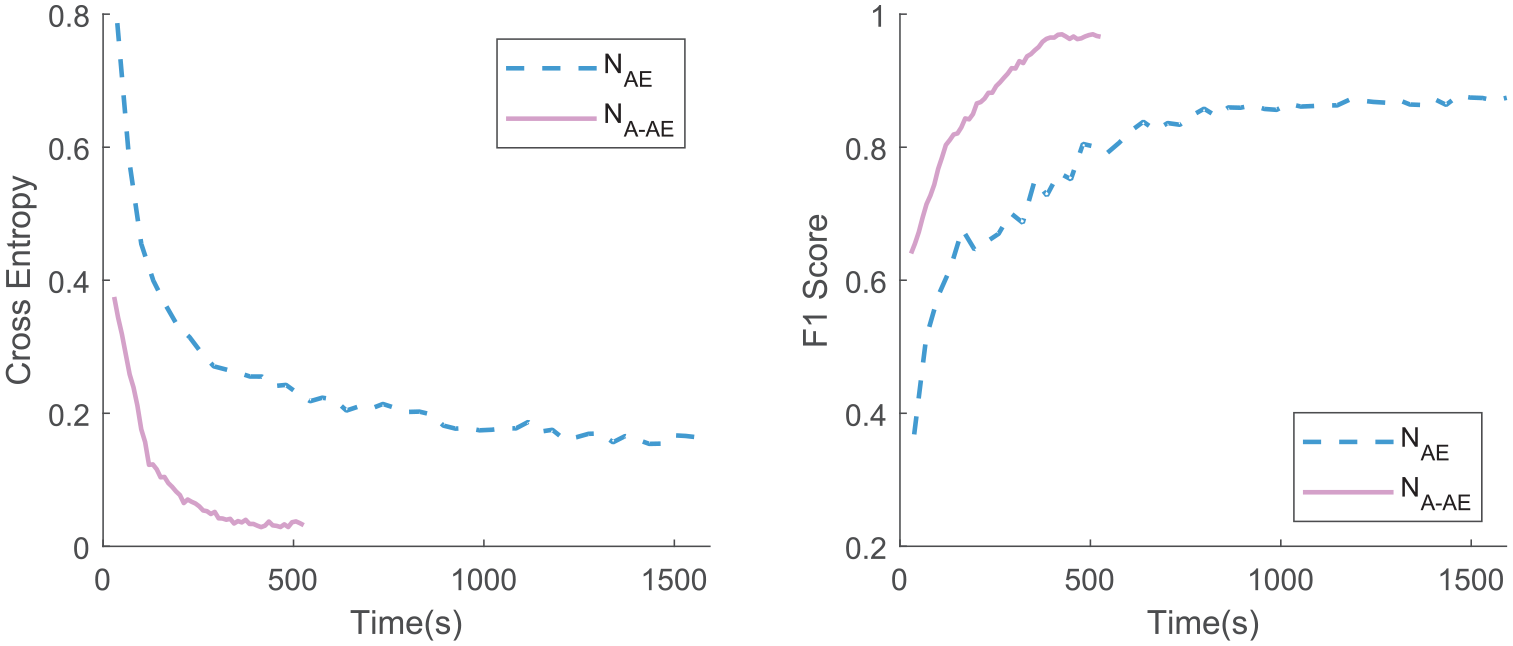
To demonstrate the effectiveness of TL, the training processes with and without TL were traced and shown in this section. One-ninth training data (320 samples) were taken out as a separate validation set during the training. The cost (cross entropy) and the F1 score on the validation set were measured when each epoch of training is finished. The results of 50 epochs are shown in Figure 17.

Figure 17.

Training progress of N_AE and N_A-AE on the validation set.

It is found that the N_A-AE can learn to reduce the validation cost much faster than N_AE since it has much fewer parameters to be tuned. Without calculation details given, the number of parameters in N_AE to be trained is 4,527,732, while this number in N_A-AE is only 65,860. To achieve an acceptable cost lower than 0.2, the N_AE requires around 700 s, which is seven times the time of N_A-AE. Although 700 s seems to be acceptable, this only corresponds to one rail turnout zone in this study. Once AE-monitoring systems are implemented in a large scale, considering numerous rail turnouts with various operating environments, passing trains and rail conditions, computation efficiency is extremely vital in quickly establishing corresponding models in time.

Even neglecting the time limit, the cost curve of N_AE eventually converges at a higher level than N_A-AE. This is owing to the overfitting problem. The model volume is relatively large in comparison with the training size, and its continuous learning on the training set is not helpful for its performance on the validation set, as well as the unseen testing set. Although the F1 score on the training set is almost 100%, on the unseen testing set, the N_AE only shows moderate performance with macro-F1 of 87.5%. As mentioned in the section “Performance comparison,” the F1 score on the testing set reaches 97.5% using N_A-AE.

Conclusion and future work

In this study, a TL approach has been developed using in-situ AE monitoring data and a pre-trained model from an audio source. In summary, the study contains three primary contributions. (1) The approach is able to evaluate the structural conditions of in-service rail tracks in a progressive manner from intact to critically cracked, as an advancement of crack detection in the authors’ previous work. It enables alarming of rail cracks at early stages and would help rail operators to conduct in-time maintenance work. (2) Compared to conventional CNN models, the proposed CNN model (N_A-AE) transfers lower-layer knowledge from a pre-trained AudioSet model, to help extract the acoustic-specific features of the time–frequency spectrograms of two months AE monitoring data collected from an in-service point rail, and only higher layers of the proposed model needs to be trained. To the authors’ knowledge, it is the first time we use massive audio recordings as “acoustic-homologous” source data to AE-based SHM evaluation. Testing results demonstrate that the developed model N_A-AE performs well on the rail condition assessment task based on AE data, with a high macro-F1 score of 97.5% and relatively short computation time. While subject to the lack of training data amount and overfitting problem, the model learning from scratch (N_AE) has a macro-F1 score of 87.5% and tripled computation time. Although the advantage of TL computation efficiency is not obvious in this study for one rail turnout, it will definitely be manifested upon numerous operating rail lines implemented with monitoring systems. (3) The closeness between source data (ImageNet, AudioSet) and the target AE monitoring data are quantitatively determined with a metric MMD, and the influence of different source data on the learning performance is investigated. It is found that the training model with knowledge transferred from images has no positive or even negative influence on the performance with a result of 86.1% macro-F1 score. This result aligns with the image-AE data MMD values, which are obviously higher than those between audio data and AE monitoring data under different calculating Kernel functions. The study provides a suggestion that when using TL in SHM evaluation, selecting source data correspondingly and appropriately would be necessary facing heterogenous monitoring data in varying SHM scenarios. It should be noted that the AE technique can only monitor a small portion of any rail. Therefore, it is more applicable for the critical zones of rail such as the rail turnout in this study or for critical components in other mechanical systems. For long-distance rails, some vehicle-based inspection methods may be more suitable, such as those based on track inspection trains.

Apart from the contributions listed above, several improvements can be made in our future work based on findings in this study:

In this study, the discrepancy between the source domain and target domain is measured by MMD as guidance for source domain selection. Recently, there are some inspiring research efforts on another kind of TL named domain adaptation, where the source task and the target task are exactly the same while the $P (X_{S})$ is invariant to the $P (X_{T})$ .^42,68 In this case, the MMD can be put into the cost function to boost the learning of domain-invariant features so that the well-trained classifier for the same task can be shared. Following this idea, we are working on transferring a model from one turnout to another.

Despite the excellent performance of the proposed model, the optimization of hyperparameters is still worth investigating, such as the optimum layer to be unfrozen. Besides, the window width of STFT on acoustic waveforms can also be further studied for a better representation. Moreover, it is worth looking into whether using more relevant data categories (crackle, crack, shatter) available on AudioSet as source data rather than the entire database will achieve better evaluation performance on rail crack identification.

The clustering phenomenon of visualized bottleneck features is observed in Figure 12(c) where the AE data from healthy turnout exhibit obvious borders from other conditions. This provides a possibility of unsupervised learning, and it is expected that rail condition evaluation can be conducted even when only healthy data are available. Histogram-based Outlier Score (HBOS)⁶⁹ and k Nearest Neighbors (KNN) are all potentially effective algorithms for this, and the authors are currently researching into this.

Footnotes

Declaration of conflicting interests

The author(s) declared no potential conflicts of interest with respect to the research, authorship, and/or publication of this article.

Funding

The author(s) disclosed receipt of the following financial support for the research, authorship, and/or publication of this article: This research was funded by a grant (RIF) from the Research Grants Council of the Hong Kong Special Administrative Region, China (Grant No. R5020-18). This research was also funded by the grants from the Ministry of Science and Technology of China and the Innovation and Technology Commission of Hong Kong SAR Government to the Hong Kong Branch of Chinese National Rail Transit Electrification and Automation Engineering Technology Research Center (Grant No. K-BBY1).

ORCID iDs

Si-Xin Chen

Lu Zhou

Yi-Qing Ni

References

McCrory

Al-Jumaili

Crivelli

, et al. Damage classification in carbon fibre composites using acoustic emission: a comparison of three techniques. Compos Part B Eng 2015; 68: 424–430.

Thomas

H-M

Junger

Hintze

, et al. Pioneering inspection of railroad rails with eddy currents. In: Proceedings of 15th world conference on non-destructive testing (WCNDT), Roma, 15–21 October 2000.

Clark

. Rail flaw detection: overview and needs for future developments. NDT E Int 2004; 37(2): 111–118.

Ph Papaelias

Roberts

Davis

. A review on non-destructive evaluation of rails: State-of-the-art and future development. Proc IMechE, Part F: J Rail and Rapid Transit 2008; 222(4): 367–384.

Zhou

Brunskill

Lewis

. Real-time non-invasive measurement and monitoring of wheel-rail contact using ultrasonic reflectometry. Struct Health Monit 2019; 18(5–6): 1953–1965.

Rose

Avioli

Mudge

, et al. Guided wave inspection potential of defects in rail. NDT E Int 2004; 37(2): 153–161.

Loveday

. Guided wave inspection and monitoring of railway track. J Nondestruct Eval 2012; 31(4): 303–309.

Bartoli

di Scalea

Fateh

, et al. Modeling guided wave propagation with application to the long-range defect detection in railroad tracks. NDT E Int 2005; 38(5): 325–334.

Di Scalea

Rizzo

Coccia

, et al. Non-contact ultrasonic inspection of rails and signal processing for automatic defect detection and classification. Insight—Non-Destruct Test Cond Monit 2005; 47(6): 346–353.

10.

Shen

Cesnik

. Local interaction simulation approach for efficient modeling of linear and nonlinear ultrasonic guided wave active sensing of complex structures. J Nondestruct Eval Diagnost Prognost Engineering Systems 2018; 1(1): 84–94.

11.

Papaelias

Lugg

Roberts

, et al. High-speed inspection of rails using ACFM techniques. NDT E Int 2009; 42(4): 328–335.

12.

Molodova

Nunez

, et al. Automatic detection of squats in railway infrastructure. IEEE Trans Intell Transp Syst 2014; 15: 1980–1990.

13.

Oregui

Carroll

, et al. Detection of bolt tightness of fish-plated joints using axle box acceleration. In: Proceedings of 1st international conference on railway technology: research, development and maintenance, Sheffield, 11–20 April 2012. Civil-Comp Press.

14.

Salvador

Naranjo

Insa

, et al. Axlebox accelerations: their acquisition and time–frequency characterisation for railway track monitoring purposes. Measurement 2016; 82: 301–312.

15.

Bruzelius

Mba

. An initial investigation on the potential applicability of acoustic emission to rail track fault detection. NDT E Int 2004; 37(7): 507–516.

16.

Thakkar

Steel

Reuben

. Rail–wheel interaction monitoring using acoustic emission: a laboratory study of normal rolling signals with natural rail defects. Mech Syst Signal Process 2010; 24: 256–266.

17.

Yilmazer

Amini

Papaelias

. The structural health condition monitoring of rail steel using acoustic emission techniques. In: Proceedings of 51st annual conference of the British Institute of non-destructive testing 2012, Northamptonshire, 11–13 September 2012, pp. 1–12. The British Institute of Non-Destructive Testing (BINDT).

18.

Kostryzhev

Davis

Roberts

. Detection of crack growth in rail steel using acoustic emission. Ironmak Steelmak 2013; 40(2): 98–102.

19.

Zhou

Y-Q

Chen

S-X

, et al. Sensing solutions for assessing and monitoring high-speed railroads. In: Wang

Lynch

Sohn

(eds) Sensor technologies for civil infrastructures, Volume 2: applications in structural health monitoring, Edition II. Cambridge: Elsevier, in Press.

20.

Liu

X-Z

Y-Q

W-L

, et al. AET-based pattern recognition technique for rail defect detection. In: Proceedings of structural health monitoring 2015, Stanford, CA, 7–9 December 2015, pp. 561–563.

21.

Wang

Liu

. A Bayesian probabilistic approach for acoustic emission-based rail condition assessment. Comput Civ Infrastruct Eng 2018; 33(1): 21–34.

22.

LeCun

Bengio

Hinton

. Deep learning. Nature 2015; 521(7554): 436–444.

23.

Schmidhuber

. Deep learning in neural networks: an overview. Neural Netw 2015; 61: 85–117.

24.

Widodo

Yang

Kim

, et al. Fault diagnosis of low speed bearing based on acoustic emission signal and multi-class relevance vector machine. Nondestruct Test Eval 2009; 24(4): 313–328.

25.

Pandya

Upadhyay

Harsha

. Fault diagnosis of rolling element bearing with intrinsic mode function of acoustic emission data using APF-KNN. Expert Syst Appl 2013; 40(10): 4137–4145.

26.

Bao

Chen

Wei

, et al. The state of the art of data science and engineering in structural health monitoring. Engineering 2019; 5(2): 234–242.

27.

Bao

Chen

, et al. Surface fatigue crack identification in steel box girder of bridges by a deep fusion convolutional neural network based on consumer-grade camera images. Struct Health Monit 2019; 18(3): 653–674.

28.

Donahue

Jia

Vinyals

, et al. DeCAF: a deep convolutional activation feature for generic visual recognition. In: Proceedings of the 31st international conference on machine learning (ICML2014), Beijing, China, 22–24 June 2014.

29.

Bae

Choi

Kim

. Acoustic scene classification using parallel combination of LSTM and CNN. In: Proceedings of the detection and classification of acoustic scenes and events 2016 workshop (DCASE2016), Budapest, 3 September 2016, pp. 11–15. Tampere University of Technology.

30.

Schlüter

Böck

. Improved musical onset detection with convolutional neural networks. In: Proceedings of 2014 IEEE international conference on acoustics, speech and signal processing (ICASSP 2014), Florence, 4–9 May 2014, pp. 6979–6983.

31.

Zhang

Stewart

Entezami

, et al. Intelligent acoustic-based fault diagnosis of roller bearings using a deep graph convolutional network. Measurement 2020; 156: 107585.

32.

Sanchez

R-V

Zurita

, et al. Gearbox fault diagnosis based on deep random forest fusion of acoustic and vibratory signals. Mech Syst Signal Process 2016; 76–77: 283–293.

33.

, et al. Gear pitting fault diagnosis using integrated CNN and GRU network with both vibration and acoustic emission signals. Appl Sci 2019; 9(4): 768.

34.

Ebrahimkhanlou

Salamone

. Single-sensor acoustic emission source localization in plate-like structures using deep learning. Aerospace 2018; 5: 50.

35.

Ebrahimkhanlou

Dubuc

Salamone

. A generalizable deep learning framework for localizing and characterizing acoustic emission sources in riveted metallic panels. Mech Syst Signal Process 2019; 130: 248–272.

36.

Zhang

Wang

, et al. An improved method of rail health monitoring based on CNN and multiple acoustic emission events. In: Proceedings of 2017 IEEE international instrumentation and measurement technology conference (I2MTC), Torino, 2017, pp. 1–6. New York: IEEE.

37.

Wang

Yan

, et al. Acoustic emission wave classification for rail crack monitoring based on synchrosqueezed wavelet transform and multi-branch convolutional neural network. Struct Health Monit. Epub ahead of print 1 June 2020. DOI: 1475921720922797.

38.

Yosinski

Clune

Bengio

, et al. How transferable are features in deep neural networks? In: Proceedings of advances in neural information processing systems 27 (NIPS2014), Montréal, QC, Canada, 8–13 December 2014, pp. 3320–3328. Curran Associates, Inc.

39.

Gao

Mosalam

. Deep transfer learning for image-based structural damage recognition. Comput Civ Infrastruct Eng 2018; 33(9): 748–768.

40.

Simonyan

Zisserman

. Very deep convolutional networks for large-scale image recognition. In: Proceedings of international conference on learning representations 2014 (IRLR2014), Banff, AB, Canada, 14–16 April 2014.

41.

Deng

Dong

Socher

, et al. Imagenet: a large-scale hierarchical image database. In: Proceedings of 2009 IEEE conference on computer vision and pattern recognition (CVPR2009), Miami, FL, 20–25 June 2009, pp. 248–255. New York: IEEE.

42.

Gardner

Liu

Worden

. On the application of domain adaptation in structural health monitoring. Mech Syst Signal Process 2020; 138: 106550.

43.

Pan

Yang

. A survey on transfer learning. IEEE Trans Knowl Data Eng 2010; 22(10): 1345–1359.

44.

Ghifary

Kleijn

Zhang

. Domain adaptive neural networks for object recognition. In: Proceedings of 13th Pacific Rim international conference on artificial intelligence (PRICAI2014), Gold Coast, QLD, Australia, 1–5 December 2014, pp.898–904. New York: Springer.

45.

Long

Cao

Wang

, et al. Learning transferable features with deep adaptation networks. In: Proceedings of the 32nd international conference on international conference on machine learning (ICML2015), Lille, 6–11 July 2015, pp.97–105. The Journal of Machine Learning Research (JMLR).

46.

Gretton

Borgwardt

Rasch

, et al. A kernel two-sample test. J Mach Learn Res 2012; 13: 723–773.

47.

Berlinet

Thomas-Agnan

. Reproducing kernel Hilbert spaces in probability and statistics. New York: Springer, 2011.

48.

Hofmann

Schölkopf

Smola

. Kernel methods in machine learning. Ann Stat 2008; 56: 1171–1220.

49.

Zhou

Liu

. Contemporary inspection and monitoring for high-speed rail system. In: Yaghoubi

(ed.) High-speed Rail. London: Intechopen, 2019. Available at: https://www.intechopen.com/books/high-speed-rail/contemporary-inspection-and-monitoring-for-high-speed-rail-system.

50.

Ansell

Blom

. Fatigue: damage tolerance design. Encyclop Mater Sci Tech 2011; 2011: 2906–2910.

51.

Sandström

Ekberg

. Predicting crack growth and risks of rail breaks due to wheel flat impacts in heavy haul operations. Proc IMechE, Part F: J Rail and Rapid Transit 2009; 223(2): 153–161.

52.

Hillmansen

Smith

. The management of fatigue crack growth in railway axles. Proc IMechE, Part F: J Rail and Rapid Transit 2004; 218(4): 327–336.

53.

Chen

Yuan

Qiu

, et al. On-line prognosis of fatigue crack propagation based on Gaussian weight-mixture proposal particle filter. Ultrasonics 2018; 82: 134–144.

54.

Chowdhury

Sehitoglu

. Mechanisms of fatigue crack growth–a critical digest of theoretical developments. Fatigue Fract Eng Mater Struct 2016; 39(6): 652–674.

55.

Verstraete

Ferrada

Droguett

, et al. Deep learning enabled fault diagnosis using time-frequency image analysis of rolling element bearings. Shock Vib 2017; 2017: 1–17.

56.

Gemmeke

Ellis

DPW

Freedman

, et al. Audio set: an ontology and human-labeled dataset for audio events. In: Proceedings of 2017 IEEE international conference on acoustics, speech and signal processing (ICASSP), New Orleans, LA, 5–9 March 2017, pp.776–780. New York: IEEE.

57.

Karthik

. class_labels_indices, https://github.com/IBM/audioset-classification/blob/master/audioset_classify/metadata/class_labels_indices.csv

58.

Piczak

. ESC: dataset for environmental sound classification. In: Proceedings of the 23rd ACM international conference on multimedia, Brisbane, QLD, Australia, 26–30 October 2015, pp. 1015–1018.

59.

Zhang

Ren

, et al. Deep residual learning for image recognition. In: Proceedings of the 29th IEEE conference on computer vision and pattern recognition (CVPR), Las Vegas, NV, 27–30 June 2016, pp. 770–778. New York: IEEE.

60.

Hershey

Chaudhuri

Ellis

DPW

, et al. CNN architectures for large-scale audio classification. In: Proceedings of 2017 IEEE international conference on acoustics, speech and signal processing (ICASSP), New Orleans, LA, 5–9 March 2017, pp. 131–135. New York: IEEE.

61.

Kumar

Khadkevich

Fugen

. Knowledge transfer from weakly labeled audio using convolutional neural network for sound events and scenes. In: Proceedings of 2018 IEEE international conference on acoustics, speech and signal processing (ICASSP), Calgary, AB, Canada, 15–20 April 2018, pp. 326–330. Institute of Electrical and Electronics Engineers (IEEE).

62.

Ioffe

Szegedy

. Batch normalization: accelerating deep network training by reducing internal covariate shift. In: Proceedings of the 32nd international conference on international conference on machine learning (ICML2015), Lille, 6–11 July 2015, pp. 448–456. The Journal of Machine Learning Research (JMLR).

63.

Nair

Hinton

. Rectified linear units improve restricted Boltzmann machines. In: Proceedings of the 27th international conference on machine learning (ICML-10), Haifa, 21–24 June 2010, pp.807–814.

64.

Kohavi

. A study of cross-validation and bootstrap for accuracy estimation and model selection. In: Proceedings of the 14th international joint conference on artificial intelligence (IJCAI95), San Francisco, CA, 20–25 August, 1995, pp.1137–1143. Morgan Kaufmann Publishers Inc.

65.

Srivastava

Hinton

Krizhevsky

, et al. Dropout: a simple way to prevent neural networks from overfitting. J Mach Learn Res 2014; 15: 1929–1958.

66.

Kingma

. Adam: a method for stochastic optimization. In: Proceedings of International conference on learning representations 2015 (ICLR 2015), San Diego, CA, 7–9 May 2015.

67.

Van Der Maaten

Hinton

. Visualizing data using t-SNE. J Mach Learn Res 2008; 9: 2579–2605.

68.

Yang

Lei

Jia

, et al. An intelligent fault diagnosis approach based on transfer learning from laboratory bearings to locomotive bearings. Mech Syst Signal Process 2019; 122: 692–706.

69.

Goldstein

Dengel

. Histogram-based outlier score (HBOS): a fast unsupervised anomaly detection algorithm. In: Proceedings of the 35th annual German conference on artificial intelligence (KI 2012), Saarbrücken, 24–27 September 2012.

An acoustic-homologous transfer learning approach for acoustic emission–based rail condition evaluation

Abstract

Keywords

Introduction

TL and MMD

In-situ AE-based monitoring system

Monitoring system

Data description

Methodologies

Time–frequency representation

Selection of source domain

Construction of A-AE TL model

Frozen layers

Segment integration and trainable layers

Baseline methods

MMD calculation

Results and discussion

Performance comparison

MMD comparison

Visualization of bottleneck features

Computation time comparison

Conclusion and future work

Footnotes

Declaration of conflicting interests

Funding

ORCID iDs

References