Sage Journals: Discover world-class research

Abstract

Flood-induced scour is among the most common external causes of bridge failures worldwide. In the United States, scour is the cause of 22 bridges fails every year, whereas in the UK, it contributed significantly to the 138 collapses of bridges in the last century. Scour assessments are currently based on visual inspections, which are time-consuming and expensive. Nowadays, sensor and communication technologies offer the possibility to assess in real time the scour depth at critical bridge locations; yet, monitoring an entire infrastructure network is not economically feasible. A way to overcome this limitation is to instal scour monitoring systems at critical bridge locations, and then extend the piece of information gained to the other assets exploiting the correlations present in the system. In this article, we propose a scour hazard model for road and railway bridge scour management that utilises information from a limited number of scour monitoring systems to achieve a more confined estimate of the scour risk for a bridge network. A Bayesian network is used to describe the conditional dependencies among the involved random variables and to update the scour depth distribution using data from monitoring of scour and river flow characteristics. This study constitutes the first application of Bayesian networks to bridge scour risk assessment. The proposed probabilistic framework is applied to a case study consisting of several road bridges in Scotland. The bridges cross the same river, and only one of them is instrumented with a scour monitoring system. It is demonstrated how the Bayesian network approach allows to significantly reduce the uncertainty in the scour depth at unmonitored bridges.

Keywords

Underwater scour structural health monitoring Bayesian inference Bayesian network bridge management

Introduction and background

Scour is defined as the excavation of material around bridge foundations as a result of the erosive action of flowing water. The phenomenon is usually classified into three different types, namely, degradation, constriction (or contraction) and local scour,¹ which generally work simultaneously to give the total scour.² When the depth of scour develops significantly, the load-bearing capacity of bridge foundations may be severely compromised, leading to structural instability and ultimately catastrophic failure.³

Flood-induced scour is among the main causes of bridge collapses, resulting in significant loss of life, traffic disruption and economic losses.⁴ In the United States, a review of 1502 river crossing failures occurring in the period 1966–2005 has shown that an average annual rate of 22 bridges were closed or failed due to scour.⁵ In the UK, there are more than 60,000 highway and railway bridges crossing waterways⁶ and almost 95,000 spans and culverts are susceptible to scour processes. According to van Leeuwen and Lamb,⁷ abutment and pier scour were responsible of 138 rail bridge failures recorded in the UK during the period 1846–2013. In the past decade in Cumbria, a non-metropolitan county in North-West England, more than 100 bridges were damaged or destroyed (e.g. the Northside bridge in 2009 and the Pooley bridge in 2015 were washed away).^8,9 Furthermore, the winter storms of 2015 resulted in severe damage to bridges across Scotland and other parts of England.¹⁰ This includes the Lamington viaduct, which resulted in the closure of the West Coast mainline between Glasgow and London for nearly 2 months due to a scour failure at one of its piers.¹¹

The scour risk assessment is a crucial element of any bridge management system. This evaluation should combine information on the hazard, the bridge vulnerability and the consequences of failure.¹² Regardless of the approach employed, an accurate estimation of the scour hole at the foundations of bridge piers and abutments is at the base of any scour vulnerability and risk assessment.¹³ Studies over the past four decades have provided several methods for the estimation of scour depth (see, e.g. Pizarro et al.¹⁴ for a state-of-the-art review), which include empirical formulas fitted to experimental data,^3,15 theoretically based formula¹⁶ and numerical approaches involving, for example, artificial neural networks.^17,18 However, most of these approaches (e.g. especially the empirical model based on lab experiments) follow the assumption that the designed flood acts over an infinite duration,¹⁴ while real flood events are characterised by hydrographs of different duration and magnitude, resulting in non-stationary hydraulic conditions that influence the scour evolution.^19,20 Moreover, the risk of failure due to scour cannot be directly related to only one designed flood scenario.²¹ Hence, comparisons between scour estimates according to the mentioned methods and actual scour depths observed on site have shown that the first may be significantly biased on the conservative side.²² This could be explained by the extreme complexity of the scour evaluation, which involves many aleatoric and epistemic uncertainties.²³ Probabilistic frameworks have been presented over the years to incorporate the effect of these uncertainties.^22–25

In the UK, Network Rail (NR) and Transport Scotland (TS) assess the risks associated with scour on road and railway bridges using the Procedures BD97/12²⁶ and EX2502,²⁷ respectively. Both these procedures rely on visual inspections, carried out at regular intervals or after major flood events, to identify the bridges that may be at risk of scour. More detailed assessments are then carried out for these bridges, and the scour depth is estimated through empirical formulas in order to produce a scour-vulnerability index (i.e. expressed as the ratio between the total scour depth at the base of the pier D_T and the foundation depth D_F) used to rate the bridge assets and prioritise scour risk mitigation interventions. The risk assessment is, therefore, based on an essentially deterministic approach, with a prefixed flood scenario (e.g. the 1 in 200 years flood).

Although visual inspections are a predominant non-destructive evaluation technique to check the state of any bridge component, they have clear disadvantages in the context of scour risk assessment. Their reliability depends on the inspector’s experience and on the equipment provided, and above all they are, in general, expensive and time-consuming. Furthermore, it is too dangerous to carry out underwater visual inspections during the peak of a flood event, when the risk of scour is the highest.

Nowadays, a wide range of sensor and communication technologies offer the possibility to assess in real time the scour depth at bridge foundations.²⁸ This could help to overcome the limitations of visual inspections, by increasing the identification of the bridges most at risk of scour. However, monitoring an entire infrastructure network is not economically sustainable, and for this reason, scour sensors may be installed only at a few critical bridges.

Hence, for these reasons, current scour risk assessment approaches could be improved by (1) explicitly considering the various sources of uncertainty that affect the problem, thus enabling the shift from a deterministic to a probabilistic evaluation of the scour depth and (2) incorporating the observations from scour sensors, allowing the reduction of the uncertainty in the scour risk estimates.

This article illustrates a probabilistic framework for the assessment of the scour hazard of bridges in a network, which is capable to use the data from scour monitoring systems installed only at critical bridge locations to improve the scour assessment for unmonitored locations within the same bridge network. In particular, the proposed framework is based on a Bayesian network (BN), which describes the conditional dependencies among the random variables (RVs) involved in the scour depth assessment at different bridges. Once a new observation on the scour depth or the flow discharge is available at a location, the BN is exploited to estimate and update the scour depth at unmonitored locations. It is noteworthy that a preliminary development of the BN for scour estimation was presented in Maroni et al.²⁹ In that article, a highly simplified BN was considered to test and compare the effectiveness of two different numerical algorithms for the Bayesian updating, namely, an algorithm to solve linear Gaussian BNs and the transitional Markov chain Monte Carlo (TMCMC) method. This article describes an extended version of this BN, integrating improved scour estimation models and better-defined sources of inherent uncertainty. To the authors’ knowledge, it constitutes the first application of BNs to bridge scour risk management.

The rest of the article is organised as follows: Section ‘Bayesian statistical inference and model updating’ outlines the principal concepts of the Bayesian logic and BN. Section ‘BN for scour estimation’ illustrates the developed BN, the involved RVs and the models employed to describe their conditional dependency. The section also explains how the BN is fed with observations from various monitoring systems and how this new information updates the variables of the network. Section ‘Numerical algorithm for model updating’ briefly describes the numerical algorithm employed to solve the BN and update the variables involved in the scour estimation. In section ‘Case study’, we present and describe the case study used to demonstrate the functioning of the BN, consisting of bridges managed by TS in South-West Scotland. These bridges cross the same river and scour depths are assumed to be monitored only in one of them. The outcomes of the application of the proposed framework to the case study are shown in section ‘Results’. The article ends with conclusions and future works in section ‘Conclusion’.

Bayesian statistical inference and model updating

The last three decades have seen a growing trend towards the development of sensor technologies and techniques for processing the data and assess the performance of civil infrastructure under environmental conditions. Bayesian inference provides a general, rational and robust approach for evaluating the structure condition (e.g. damaged or undamaged) or judge sensor and model performances, by taking into account all the sources of uncertainty relevant to the problem. Usually, information about a monitored structure might come from different sources, such as observations collected by sensors, design documentation of the structure, inspections and test reports or engineering judgement.³⁰ The inverse problem of estimation of the parameters of a model is tackled by treating them as uncertain and using available data to update their probabilistic distribution. Hence, this approach constitutes an accumulation of knowledge.³¹

Equation (1) illustrates the expression of the Bayes’ theorem for the problem of updating of state variables distribution

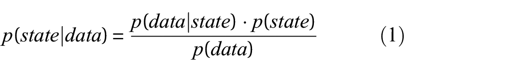
p (state | data) = \frac{p (data | state) \cdot p (state)}{p (data)}

(1)

where the probability p(state) is called prior probability and represents the perspective of the state prior to the collection of data. The probability p(data|state) is called likelihood of the observed data. Analogously, p(state|data) is called the posterior probability of the state because it is the updated belief after new information is gained through observed data. The dominator p(data) is a normalising factor called evidence, which must be calculated by integrating over the parameter space through application of the total probability theorem.

Bayesian methods have received increased attention across a number of disciplines in recent years; in particular, they have been successfully implemented in structural health monitoring (SHM) problems.^32–34 Consequently, there has been an increased interest in the use of graphical models, such as BNs, to enable Bayesian model updating in complex and large-scale problems.

Bayesian network

A BN, developed by Judea Pearl in 1985, is a graphical model using a directed acyclic graph to represent a set of RVs and their conditional dependencies.³⁵ Each RV, which can be discrete or continuous, is depicted by a node and the probabilistic dependency between two variables is represented by a link (Figure 1).

Figure 1.

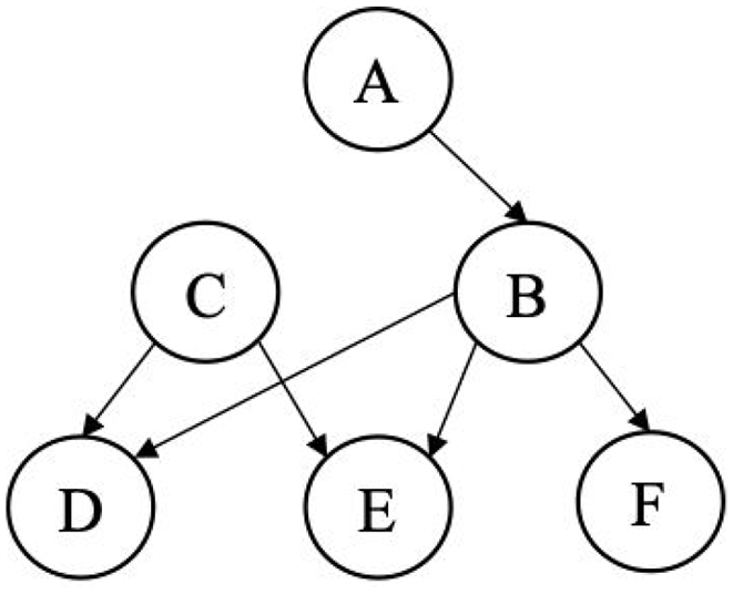
An example of a Bayesian network.

In BN terminology, it is unequivocal to refer to specific nodes as parent or child, since a directed acyclic graph represents a hierarchical arrangement. Any node extending from another one is denoted as a child, while the inverse relationship defines a parent node. Nodes without parents are known as root nodes and are described by their probability density function (pdf), which, in Bayesian terms, can be understood as their pdf.

Two forms of probabilistic inference can be carried out in BNs: predictive analysis that is based on evidence (i.e. information that the node is in a particular state) on root nodes, and diagnostic analysis, also called Bayesian learning, where observations enter into the BN through the child nodes.³⁶ The child node pdfs can be estimated from the roots’ pdfs by performing predictive analysis, whereas Bayesian learning allows updating root node pdfs when new information enters into the BN through a child node. When evidence enter into the BN, the piece of information is spread inside the network to update variable’s probabilities through one of the two forms of inference mentioned above. In particular, the second approach, the Bayesian learning, is attractive when the analysed system is based on constantly evolving information, as in the case of a real-time monitoring system. Furthermore, BNs are well suited for representing knowledge under uncertainty. Uncertainties from variables, measurements and model itself can be implemented into the BN such as components of the model or even as an updatable node.

In recent years, there has been an increasing amount of literature on the use of BNs. Although BNs were first implemented in the context of the artificial intelligence community,³⁷ they have become quickly popular in every field of study, thanks to their excellent performance and suitability for dealing with a broad range of problems that involve probabilistic reasoning and uncertainty quantification. BNs started to be used for Bayesian modelling in engineering risk analysis due to their ability to manage many dependent RVs. One of the earliest works dealing with risk assessment through the use of BNs was carried out by Friis-Hansen.³⁸ After that, several works on the employment of BN for risk assessment have been proposed starting from the article by Faber et al.,³⁹ where BNs were utilised for assessing the risk related to the decommissioning of offshore facilities. Following examples have been focused on the natural hazard risk assessment,^40–42 damage detection,^43–46 optimal sensor placement⁴⁷ and structural deterioration due to metal corrosion and fatigue using an extended version of BN that include time-variant parameters (i.e. dynamic BNs).^48,49 Dynamic BNs have been recently used to assess the time-dependent resilience of engineering systems.⁵⁰ The applications in seismic risk are many (see, for instance, Bensi et al.⁵¹) and they address different topics such as the reliability analysis of critical infrastructures in the aftermath of a hazardous event,^52,53 bridge asset⁵⁴ and road network⁵⁵ management or post-earthquake risk assessment including a decision making process.⁵⁶ BNs have been also used to evaluate multi-hazard risk.^57–60

BN for scour estimation

This section illustrates the probabilistic framework used to update the scour depths at any location of a bridge network given the data from sensors monitoring scour only at critical locations. The rationale of this framework is as follows: a scour monitoring system measures the scour depth at the pier of one bridge, and the piece of information is then extended to the other piers and the unmonitored bridges by exploiting the conditional dependence between the scour depths at different locations, as described by a BN.

The developed BN is based on BD 97/12,²⁶ which is the procedure followed by TS to assess the scour risk of their road bridges. This procedure can be divided into four steps: (1) assessment of the flow hydraulic properties, (2) estimation of the constriction scour, (3) estimation of local scour and (4) estimation of total scour. In particular, starting from the river flow characteristics (such as river flow Q), different models are applied to estimate the depth of flow upstream of the bridge y_U, and the two components of scour, constriction scour (D_C) and local scour (D_L), whose sum is equal to the total scour depth D_T. For the purpose of developing the BN, model uncertainties are added to each model to describe the randomness of the estimation processes. Thus, each formula is structured in the following way

x = f_{x} (y_{1}, \dots, y_{N}) \cdot (1 + e_{x} +^{(j)} e_{x})

(2)

where the model f_x estimates the variable x through the dependent variables y₁, …, y_N, and e_x and ^(j)e_x are the two model uncertainties: the first one represents the random error of the equation and the second one is an additional error that is associated with the specific jth location (e.g. pier or bridge). Every RV representing model uncertainty is set to be a root node of the BN and thus is described by assigning to it a prior pdf. These pdfs are expressed as normal distributions with zero mean and a standard deviation (SD). The RVs ^(j)e_x are assumed to be independent and identically distributed for the different piers. Figure 2 illustrates the BN for the problem of scour assessment at a single bridge pier. The models employed in the four steps of the assessment procedures are described more in detail in the following subsections.

Figure 2.

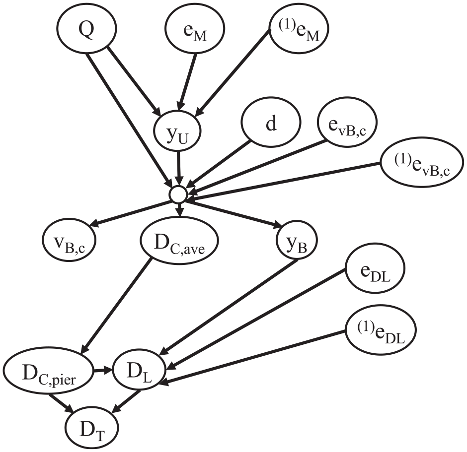
BN for scour estimation at a single bridge location.

Flow analysis

Manning equation is used to describe the relationship between Q and y_U

y_{U} = {(\frac{Q n}{B_{B} s^{1 / 2}})}^{3 / 5} (1 + e_{M} +^{(j)} e_{M})

(3)

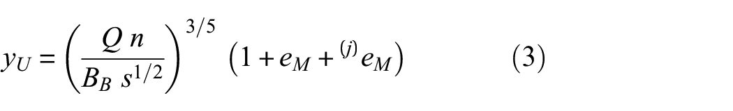
where n is the Manning coefficient, B_B is the channel width at bridge opening and s is the channel slope. Two model uncertainties are employed: e_M is the correlated model error of the Manning equation and ^(j)e_M is the uncorrelated model error in the jth bridge. The SD of each error is chosen equal to 0.10 in order to define a total SD corresponding to 0.15.

Constriction scour

The reduction of channel width due to the presence of bridge piers or abutments leads to an increase in the water velocity v_B. When the velocity reaches the critical value v_B,c (i.e. threshold velocity below which scour does not occur), the erosion of the riverbed starts.

The equilibrium (i.e. the final scour hole) is reached when the increase in cross-sectional area of flow for constriction scour is such that v_B < v_B,c.

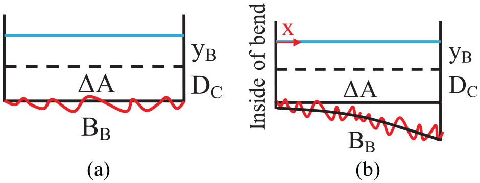
A nonlinear system of three equations in three variables is developed to estimate the constriction scour depth. Q, y_U and the bed material grain size d are the input parameters of the system that enable us to evaluate the average constriction scour D_C,ave, the water level through the bridge y_B and the threshold velocity v_B,c. The nonlinear system consists of the Colebrook–White equation (equation (4a)),¹ the conservation of fluid mass (equation (4b)) and the Bernoulli equation (equation (4c))

\begin{matrix} v_{B, c} = - \sqrt{32} v_{0} (d) \cdot lo g_{10} \\ (\frac{d}{12 (y_{B} + D_{C, ave})} + \frac{0.222 ν}{(y_{B} + D_{C, ave}) \cdot v_{0} (d)}) \\ (1 + e_{v_{B, c}} +^{(j)} e_{v_{B, c}}) \end{matrix}

(4a)

Q = v_{B, c} (y_{B} + D_{C, ave}) B_{B}

(4b)

y_{U} + \frac{{(Q / y_{U} B_{U})}^{2}}{2 g} = y_{B} + \frac{v_{B, c}^{2}}{2 g}

(4c)

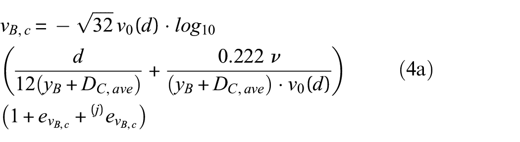
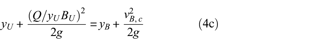
where ν is the kinematic viscosity of water and v₀(d) is the shear velocity at the threshold of movement.¹ The last two equations are considered deterministic; therefore, the model errors are added to the Colebrook–White equation alone: the correlated, $e_{v_{B, c}}$ (i.e. it is the bias of the Colebrook–White equation) and the uncorrelated error, ${{}^{(j)}e}_{v_{B, c}}$ (i.e. it is the error in the estimation in the jth bridge). The total SD is set equal to 0.15 and it is split equally between the two types of model uncertainties meaning that their SDs are equal to 0.10 each.

The previous step of the BN provides the average value of the constriction scour D_C,ave; this value is then multiplied by a factor F_S to obtain the constriction scour depth along the channel width. Table 1 provides the values of F_S according to the shape of the river and Figure 3 shows the two scenarios described in the table.

Table 1.

Constriction scour distribution factor F_S.²⁶

Location	Outside of bend	Centre of channel	Inside of bend
On or downstream of sharp bend	2.0	1.25	1.0
On or downstream of moderate bend	1.5	1.25	1.0
On straight reach	1.25	1.25	1.25

Figure 3.

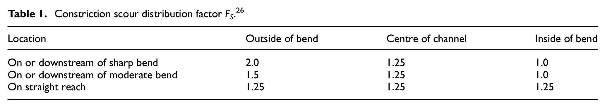
Constriction scour depth profile in a straight (a) and bended (b) reach.

In order to include all the cases of Table 1, we define the constriction scour depth at the pier D_C,pier or, generally, the constriction scour at every location of the river as

D_{C, pier} = D_{C, ave} (1 + e_{F_{S}} + e_{D_{C, ave}})

(5)

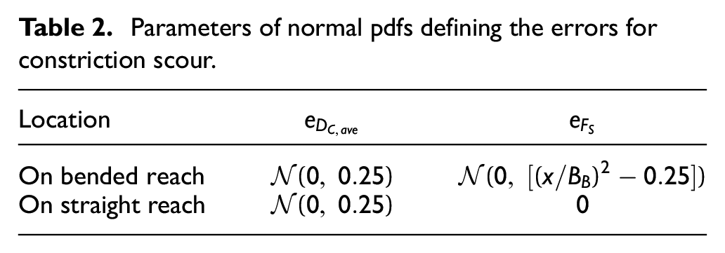
To be consistent with the structure of equation (2), two types of errors can be modelled for including the multiplication factor F_S in the estimation of D_C across the channel width. The two errors are again expressed as a normal pdf with zero mean and an SD. According to Table 1, we define $e_{D_{C, ave}}$ that is the error in the calculation of D_C,ave itself, which occurs when the reach is either straight or bended. The second error is $e_{F_{S}}$ , which takes into account the error in the scour estimation where the river bends, that is, it takes into account the additional component due to bend scour. This contribution to total scour is caused by the increase in velocity around the outside of the bend.¹ Table 2 provides the two parameters defining the normal pdf $N$ for the two errors in both limit cases.

Table 2.

Parameters of normal pdfs defining the errors for constriction scour.

Location	$e_{D_{C, ave}}$	$e_{F_{S}}$
On bended reach	$N (0, 0.25)$	$N (0, [(x / B_{B})^{2} - 0.25])$
On straight reach	$N (0, 0.25)$	0

Local scour

The formation of vortices at pier base is the principal mechanism causing the local scour,⁶¹ and the pier width W_P is the primary controlling parameter, which is corrected by some factors depending on its shape, its inclination with respect to the river flow and the local water level.

The expression of the local scour depth according to Highway Agency²⁶ is

D_{L} = 1.5 W_{P} f_{PS} f_{PA} f_{y} (1 + e_{D_{L}} +^{(j)} e_{D_{L}})

(6)

where f_PS is the shape factor, f_PA is the pier alignment factor and f_y is the flood depth factor. Two model uncertainties are again added: the correlated one, $e_{D_{L}}$ (i.e. the bias in the equation itself) and the uncorrelated one, ${{}^{(j)}e}_{D_{L}}$ (i.e. the error in the estimation in the jth pier). The total SD is set equal to 0.30 and divided equally between the two model uncertainties.

Total scour

The depth of total scour D_T is simply the sum of the two components, constriction scour depth D_C and local scour depth D_L. This expression is assumed as deterministic; consequently, no model uncertainties are added

D_{T} = D_{C} + D_{L}

(7)

It is noteworthy that, in general, the scour depth at a bridge location is also affected by the natural evolution of the riverbed. This contribution, denoted to as degradation scour, is not considered in the BD 97/12,²⁶ and for this reason, it is not explicitly modelled in the BN. However, the observations used to update the variables of the BN should reflect this component.

Bayesian learning

With reference to the presented BN, it is assumed that three quantities can be monitored, that is, the river level upstream of the bridge y_U, the total scour depth D_T, and the constriction scour $D_{C}^{*}$ in the middle of the channel. Environmental agencies can provide water level data from gauging stations, while a wide range of SHM sensors can be employed to measure scour,²⁸ such as time domain reflectometry,⁶² radar devices⁶³ or dielectric probes;^64,65 therefore, a scour monitoring system can provide data about the two scour depths. When new observations become available, the BN model is used to propagate the new piece of information through the network and update probabilities.³⁵

The solution of the BN can be broken down into three steps:

Defining the prior pdf of the root nodes (grey nodes in Figure 4(a)): water flow Q, grain size d, the correlated model uncertainties e_M, $e_{v_{B, c}}$ and $e_{D_{L}}$ and the uncorrelated ones (not displayed in Figure 4(a)). Observations of y_U, $D_{C}^{*}$ and D_T enter into the network (red nodes in Figure 4(a)).

Splitting the BN into three sub-networks to have three different updating processes: y_U updates e_M; $D_{C}^{*}$ and y_U update $e_{v_{B, c}}$ and d; D_T, y_U and $D_{C}^{*}$ (through D_C,pier) update $e_{D_{L}}$ (Figure 4(b)).

Updating the descendant nodes (light yellow nodes in Figure 4(c)).

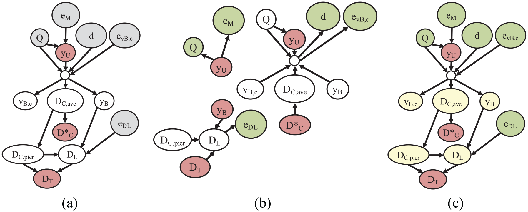
The BN can be extended to a second bridge with N piers because the scour estimation is based on the same models. For instance, Figure 5 shows a BN for scour estimation at two bridges, each of them with N piers. The estimation of the scour depth at the second bridge is based on the models corrected by the model uncertainty updated by direct observations of ${{}^{(1)}D}_{C}^{*}$ and ⁽¹⁾D_T at one pier of the first bridge. The three correlated model uncertainties are root nodes of each sub-network that represents a different bridge; these connections allow the BN to extend information gained from the scour monitoring system to each sub-network (i.e. unmonitored bridges) because the models used to estimate scour depths are the same for any bridge. Consequently, the scour estimation at every pier is affected by the same correlated error.

Figure 4.

(a) Starting with prior pdfs, (b) updating of root nodes and (c) descendant nodes.

Figure 5.

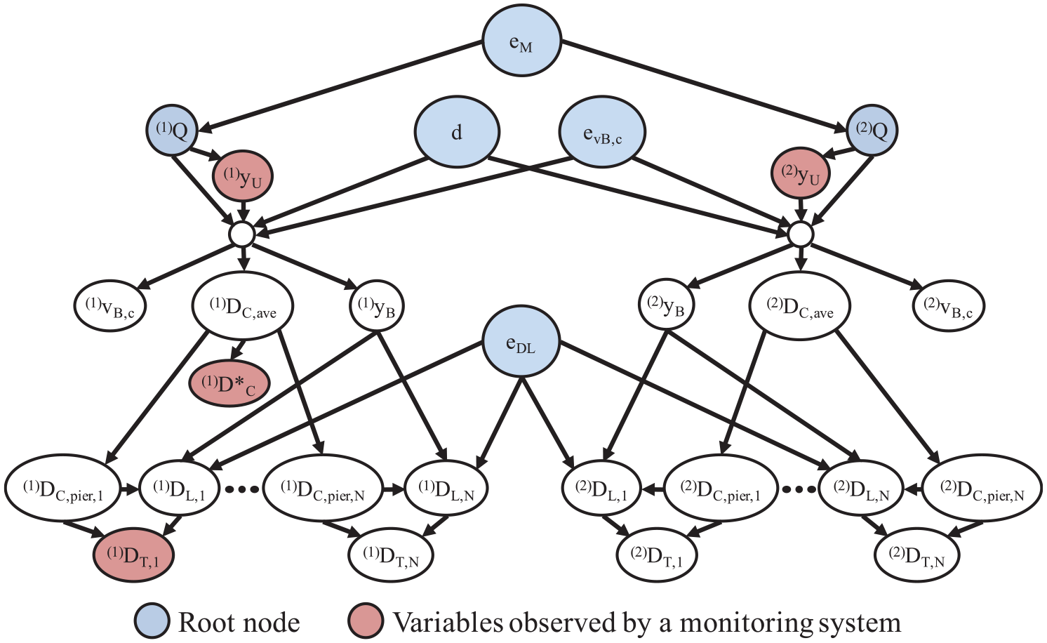
BN for scour estimation at two bridges on the same river, both with N piers.

It is worth mentioning that the above BN can be also used to perform predictive analysis, that is, the first type of inference described in section ‘BN’. As its name suggests, this analysis allows predicting the pdfs of the child nodes by starting from the prior pdfs of the parent nodes, without any observations entering the BN.

Finally, it is noteworthy that the BN could also be extended to incorporate other sources of information, such as direct river velocity measurements or forecast flood hydrographs. For this purpose, suitable hydraulic and hydrological models must be added to relate the various parameters.

Numerical algorithm for model updating

Despite the numerous advantages associated with Bayesian inference, its practical implementation involves some challenges, especially when continuous RVs are employed, as in the case of data collected by a monitoring system. A closed form solution of equation (1) is usually not available, and thus it is necessary to resort to numerical algorithms to calculate the posterior distribution’s parameters (e.g. mean value vector and covariance matrix). Given this, equation (1) can be rewritten as

p (state | data) \propto p (data | state) \cdot p (data)

(8)

The class of algorithms belonging to the Markov chain Monte Carlo (MCMC) methods⁶⁶ is a common choice when Bayesian inference must be carried on. These methods are a broad family of numerical algorithms that generate next sample values by performing a random sampling from the previous sample values. Their essential idea is using randomness to solve problems that might be deterministic in principle. Examples of these sampling methods are Monte Carlo, Metropolis–Hasting and TMCMC. These computer algorithms can be used to draw an (approximate) random sample from the posterior pdf, without having to completely evaluate it. The posterior pdf can be approximated to any accuracy level by taking a large number of samples.

The Metropolis–Hastings algorithm⁶⁷ is the most used and simple approach to make inference for Bayesian parameter estimation. It allows to extract samples from the actual posterior pdf. However, the method has some disadvantages: it does not calculate the evidence, the required number of samples N might be huge in some cases and it requires to always consider the burn-in period, that is, a period after which the samples are independent from the starting choice of the parameter to estimate. In order to overcome the issues above, the TMCMC method⁶⁸ has been proposed. In the TMCMC method, an iterative approach is used to generate samples from the unknown posterior distribution by changing the proposal pdf at each step until the target distribution is reached. Thus, n intermediate distributions p_j are considered

p_{j} \propto p {(data | state)}^{β_{j}} \cdot p (state)

(9)

where the index j denotes the step number. The likelihood function is scaled down by an exponent β_j, with 0 = β₀ < … < β_j < … < β_n = 1. It is worth noting that this construction does not alter the Bayesian logic: the series of intermediate distributions starts from the prior pdf (i.e. p₀ = p(state)) and ends with the posterior (i.e. p_n = p(state|data)). The algorithm starts at the step j by generating samples from the prior pdfs using a Monte Carlo simulation. Then, at the step j + 1, Markov chains with the Metropolis–Hasting algorithm are used to generate the p_j+₁ distribution, by choosing selected samples taken from the p_j distribution according to ‘plausibility weights’. Before advancing to the next step, β_j is updated. The algorithm stops when β_j is equal to 1.

The TMCMC method is particularly convenient for dealing with complex joint pdfs (e.g. multimodal distributions) and does not require defining any proposal distribution or removing samples in the burn-in period. In Ching and Wang,⁶⁹ a comparison is made between the TMCMC and the Metropolis–Hastings algorithm, and the advantages of the former are highlighted.

Case study

The functioning of the developed BN is demonstrated using a small bridge network, consisting of bridges managed by TS in South-West Scotland (Figure 6). The bridges cross the same river (River Nith) and only Bridge 1 is instrumented with a scour monitoring system. The aim is to exploit the observations on Bridge 1 to update the pdf of the total scour depth at other bridge locations.

Figure 6.

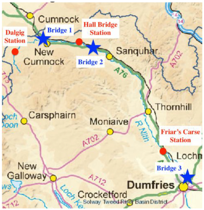
Three bridges over the River Nith. Red circles represent SEPA’s gauging stations.

Three bridges with significant scour events in the past are chosen from the TS scour database:

Bridge 1: A76 200 Nith Bridge in New Cumnock (Figure 7). It is a three-span (9.1, 10.7 and 9.1 m) stone-masonry arch bridge, with two piers in the riverbed. Both the abutments and the piers are founded on spread footings on the natural riverbed. In October 2018, a dielectric scour probe was installed on the upstream side of Pier 1 in order to measure the total scour at this pier. Moreover, another probe was installed in the centre of the channel immediately upstream of the Nith Bridge, in order to obtain a measurement of the degradation and constriction scour. The development and deployment of the scour probes are described in Maroni et al.⁶⁵

Bridge 2: A76 120 Guildhall Bridge in Kirkconnel (Figure 8). It is a three-span (8.8, 11.3 and 11.3 m) masonry arch bridge, with one pier in the riverbed. Both the abutments and the piers are founded on spread footings on natural ground, except one abutment’s spread footing that is founded on rock.

Bridge 3: A75 300 Dalscone Bridge in Dumfries (Figure 9). It is a seven-span (spans of 35 m and two of 28 m) steel–concrete composite bridge, with one pier in the riverbed. The abutments are founded on pile foundations on made up ground, while the piers are founded on pile foundations on natural ground.

The final BN for the estimation of the total scour at every bridge pier is depicted in Figure 10. The sub-networks corresponding to the three bridges are identifiable; correlated errors and the bed material grain size are root nodes in common for all bridges. The river flow Q is not a common root node because the three bridges are far apart and numerous tributaries of River Nith extend from Bridge 1 to Bridge 3. A hydrological model may be employed to correlate the river flows Q among the three sub-networks, but this is out of the scope of the article. Furthermore, there is a gauge station measuring the flow before each bridge; therefore, upstream water flow data are available for each of the bridges.

Figure 7.

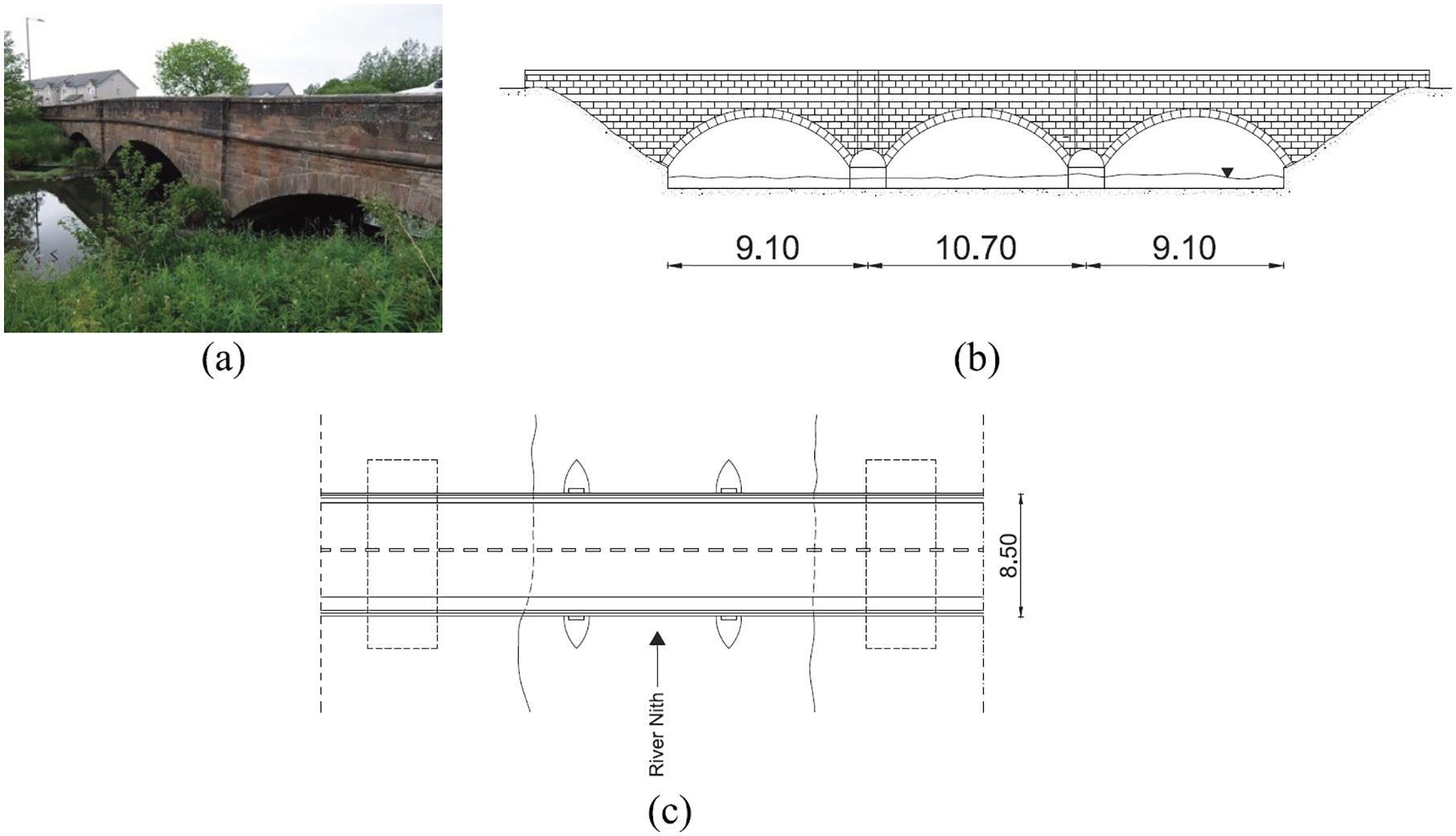
(a) A76 200 Nith Bridge, (b) bridge elevation and (c) plan view.

Figure 8.

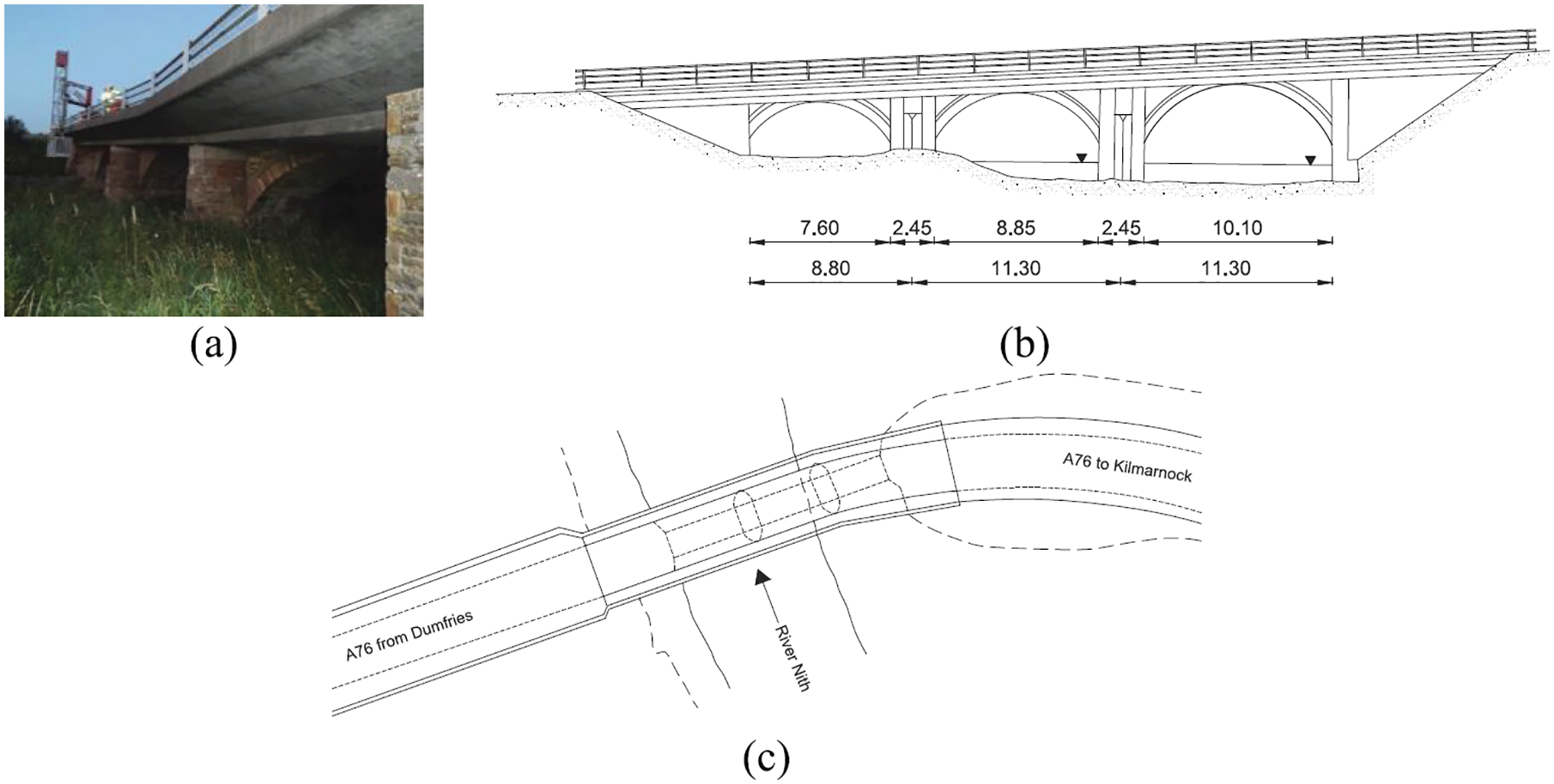
(a) A76 120 Guildhall Bridge, (b) bridge elevation and (c) plan view.

Figure 9.

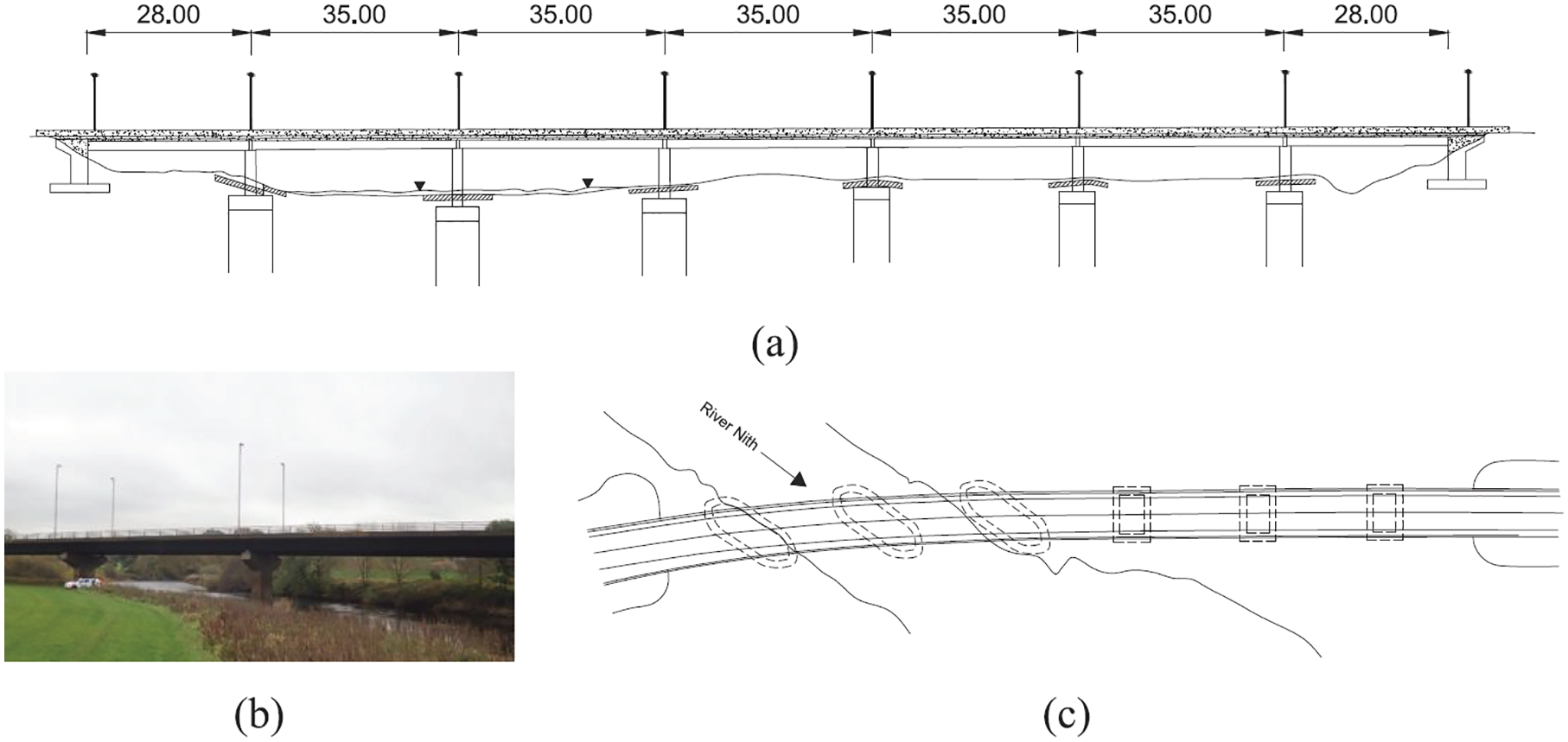
(a) Bridge elevation, (b) A75 300 Dalscone Bridge and (c) plan view.

Figure 10.

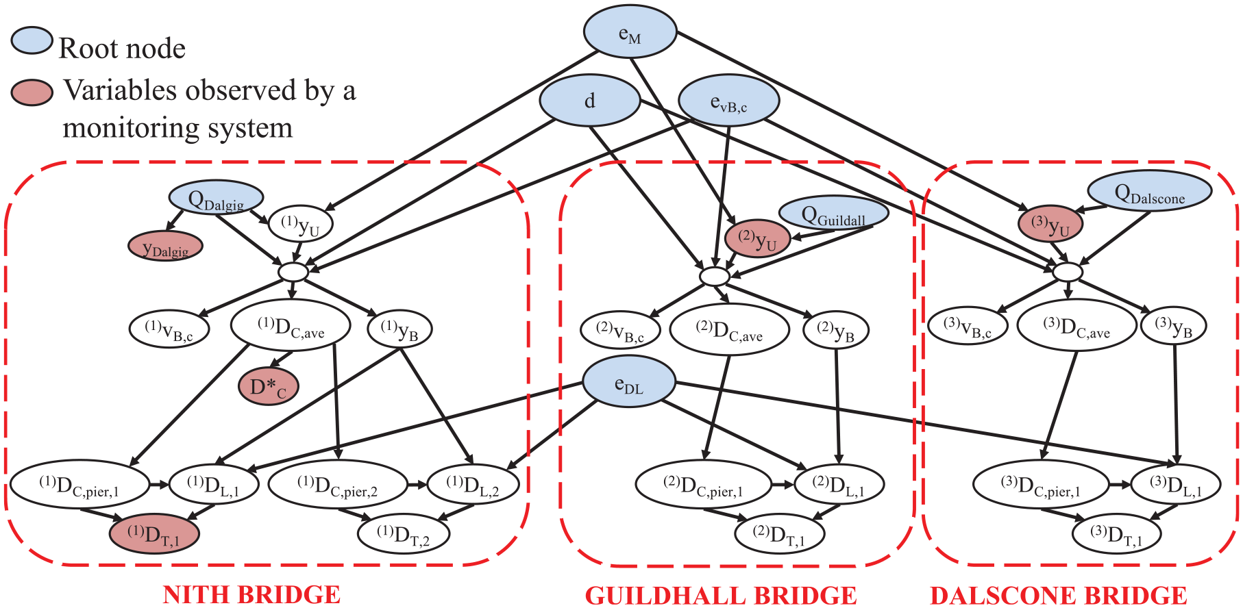
BN developed for the case study.

Results

Normal pdfs are employed for every variable except for river flows, which are described by a log-normal pdf because the discharge cannot be negative. The parameters of the log-normal pdfs (i.e. mean and SD of logarithmic values) are based on the gauging station data of the last 10 years collected by the Scottish Environmental Protection Agency (SEPA). They are shown in Table 3, while Figure 11 depicts the pdfs fitting the data. The prior pdfs of the model errors are set as normal distributions with zero mean and SDs defined previously.

Table 3.

Parameters defining the prior pdf of the flow discharge Q based on SEPA’s data.

SEPA gauging station	Bridge	μ (m³/s)	σ (m³/s)
Dalgig	Nith	−0.2810	1.1261
Hall Bridge	Guildhall	1.1426	1.2021
Friar’s Carse	Dalscone	2.9539	0.9925

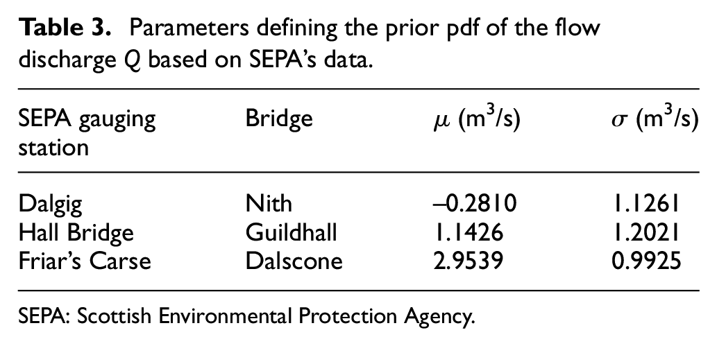
SEPA: Scottish Environmental Protection Agency.

Figure 11.

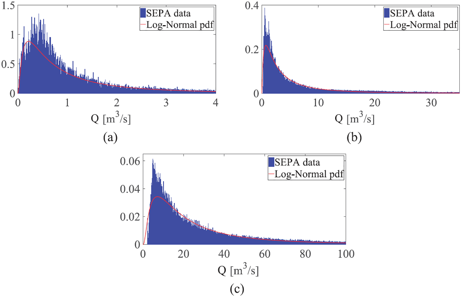
Prior log-normal pdfs of the river flow at (a) Dalgig, (b) Hall Bridge and (c) Friar’s Carse gauging station.

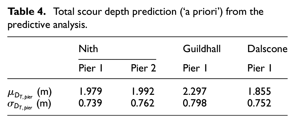
The predictive analysis is carried out by running a Monte Carlo simulation. This type of analysis requires only the parent nodes’ prior pdf and no observations enters into the BN to make a prediction of the distribution of the child nodes. A total of 10,000 samples of the root nodes pdfs is considered to estimate the prior pdf of the total scour depth D_T,pier at each pier. The mean value, $μ_{D_{T, pier}}$ , and the SD, $σ_{D_{T, pier}}$ , of the predictions are summarised in Table 4. It can be observed that the scour depth distributions at the various piers are characterised by a significant dispersion, with SD values of the order of 0.75 m.

Table 4.

Total scour depth prediction (‘a priori’) from the predictive analysis.

	Nith		Guildhall	Dalscone
	Pier 1	Pier 2	Pier 1	Pier 1
$μ_{D_{T, pier}}$ (m)	1.979	1.992	2.297	1.855
$σ_{D_{T, pier}}$ (m)	0.739	0.762	0.798	0.752

Although the scour probes installed in the A76 200 bridge provide continuous real-time scour data since 4 October 2018, no major flood events have been recorded yet. Thus, the simulation of the inference problem in the BN considers a hypothetical flood scenario compatible with the historical record of floods for the River Nith. In particular, the Bayesian learning is carried out by assuming that observations are available for the river levels y_U upstream of three bridges, the degradation and contraction scour depth at the A76 200 bridge and the total scour depth at Pier 1 of the same bridge. Table 5 shows the water level values recorded at the gauging stations, simulating a flood event with return period of about 20 years. The scour data are assumed equal to 0.20 m for constriction scour depth $D_{C}^{*}$ and 0.45 m for total scour depth D_T.

Table 5.

Case scenario for river level observations.

SEPA gauging station	Bridge	Water level (m)(30 Dec 2013)
Dalgig	Nith	1.879
Hall Bridge	Guildhall	3.015
Friar’s Carse	Dalscone	1.512

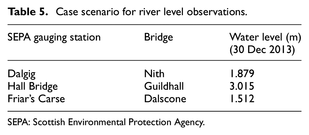
SEPA: Scottish Environmental Protection Agency.

The TMCMC algorithm⁶⁸ is then used to perform the Bayesian learning analysis and update the root nodes. Thousand samples are extracted at each stage of the TMCMC method, and this is repeated 100 times for each update to eliminate the influence of randomness. To solve the whole network, five updates have to be performed. Each update is connected to one observed variables (i.e. water flow upstream of each bridge, constriction scour depth ${{}^{(1)}D}_{C}^{*}$ and local scour depth ⁽¹⁾D_T at first bridge). Considering that each TMCMC application requires on average seven stages, the number of extracted samples, which corresponds to how many times the calculation of the likelihood function is performed, is equal to 5 × 100 × 7 × 10,000 = 3,500,000 samples.

Figure 12 shows the comparison between the results of the total scour depth D_T obtained ‘a priori’ with a Monte Carlo simulation (i.e. predictive analysis) and the estimations obtained after the Bayesian learning with the TMCMC method. With regards to A76 200 Bridge, the total scour depth at Pier 2 has a mean value equal to the one measured at Pier 1 (Figure 12(a)). This is indeed an expected result, since the piers belong to the same bridge, have the same geometry and the riverbed material and the water conditions are identical for them. However, it can be observed that while the value of the scour depth at Pier 1 is known deterministically (assuming that the measurement is affected by no uncertainty), the one at Pier 2 is uncertain, with an SD of 0.17 m. It is noteworthy that this value of SD is significantly lower than the one corresponding to the prior pdf (0.76 m). The decrease in dispersion, of about 80%, is the result of the added information and the high correlation existing between the scour depths at the two piers of the bridge. It can be observed in Figure 12(b) and (c) that the Bayesian learning also allows the updating of the estimates of the total scour depth D_T at the piers of unmonitored bridges. In fact, the mean values of the total scour depth at these piers reduce significantly. Moreover, the SDs of the posterior distributions are close to 0.21 m, which constitutes a significant increase (more than 70%) in accuracy compared to the prior estimates.

Figure 12.

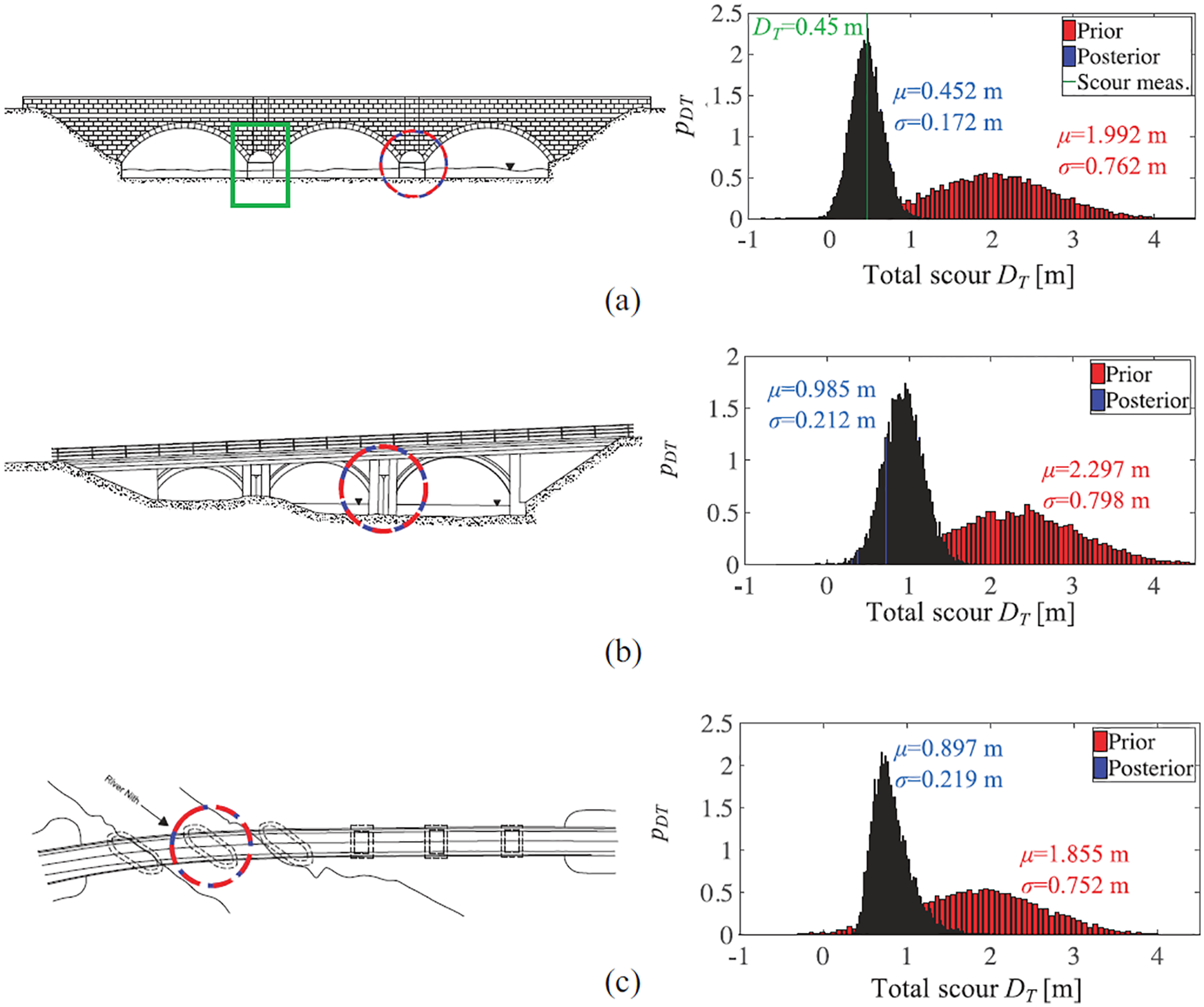
Comparison between prediction and estimation of total scour depths: (a) Pier 2 of Nith Bridge. (b) Pier 1 of Guildhall Bridge. (c) Pier 1 of Dalscone Bridge.

Conclusion

This article shows the development of a probabilistic framework for scour hazard assessment that uses limited data from monitoring systems to update the probability distribution of the scour depth at the foundations of bridges in a network. The proposed framework is based on a BN that describes the conditional dependencies between the scour depth at different piers within the same bridge or belonging to other bridges in the network. Once new observations on the river flow characteristics and/or scour data are available, Bayesian learning with the TMCMC algorithm is used to update the scour depth distribution at unmonitored locations.

A case study consisting of three bridges managed by TS in South-West Scotland is considered to demonstrate the functioning of the BN. The bridges cross the same river, and only one bridge (Bridge 1) is instrumented with a scour monitoring system. The aim is to exploit direct observations of total scour depth D_T and the constriction scour $D_{C}^{*}$ measured at Bridge 1 in order to predict the scour depth at other unmonitored piers. A flood event is simulated using river level data from gauging stations upstream of the bridges. It is shown that the available limited data from the scour monitoring system and the flow depths allow to increase significantly the accuracy of the scour estimates at unmonitored bridge piers. This increase in accuracy is in the order of 70%.

It is currently planned that the continuous real-time measurements of the scour depth at the monitored bridge locations of the Nith Bridge in New Cumnock will be fed into the developed BN to update in real time the estimates of the scour depth at other locations of the bridge network. Additional probes, installed at other locations, will be used to validate the proposed monitoring framework. Moreover, the outcomes of the presented framework will be used in a future study in combination with fragility curves to provide real-time estimates of the risk of bridge failure due to scour and inform a decision system, supporting transport agencies’ decision processes under extreme flood events. Future research will also consider the extension of the BN with structural models, allowing to incorporate also information from sensors mounted on the bridges, such as accelerometers or inclinometers.

Footnotes

Declaration of conflicting interests

The author(s) declared no potential conflicts of interest with respect to the research, authorship and/or publication of this article.

Funding

The author(s) disclosed receipt of the following financial support for the research, authorship and/or publication of this article: This study has been carried out within the project titled ‘Early warning decision support system for the management of underwater scour risk for road and railway bridges’, which has received funding from the NERC ERIIP (Environmental Risk to Infrastructure Innovation Programme) under Grant Agreement No. NE/R009090/1.

ORCID iD

Andrea Maroni

References

Kirby

Roca

Kitchen

, et al. Manual on scour at bridges and other hydraulic structures. 2nd ed. London: CIRIA, 2015.

Lauchlan

Melville

. Riprap protection at bridge piers. J Hydr Eng ASCE 2001; 127(5): 412–418.

Richardson

Davis

. Evaluating scour at bridges. 4th ed. Hydraulic engineering circular no. 18, Report no. FHWA NHI 01-001, 2001. Washington, DC: U.S. Department of Transportation, Federal Highway Administration.

Wardhana

Hadipriono

. Analysis of recent bridge failures in the United States. Perform Constr Facilit 2003; 17: 144–150.

Briaud

Brandimarte

Wang

, et al. Probability of scour depth exceedance owing to hydrologic uncertainty. Georisk 2007; 1(2): 77–88.

Clubley

Richards

Manes

. High-resolution sonars set to revolutionise bridge scour inspections. Proc Inst Civ Eng: Civ Eng 2015; 168(1): 35–42.

van Leeuwen

Lamb

. Flood and scour related failure incidents at railway assets between 1846 and 2013. Skipton: Railway Safety & Standards Board, 2014.

Cumbria Intelligence Observatory. Cumbria floods November 2009: an impact assessment, www.cumbria.gov.uk/elibrary/view.asp?id=35688 (2010, accessed 11 July 2019).

Zurich Insurance Group and JBA Trust. Flooding after storm Desmond, http://repo.floodalliance.net/jspui/handle/44111/2252 (2015, accessed 20 July 2019).

10.

Department for Transport. £40 million to help rebuild flood-hit roads for people in Cumbria and Lancashire, https://www.gov.uk/government/news/40-million-to-help-rebuild-flood-hit-roads-for-people-in-cumbria-and-lancashire (2015, accessed 11 July 2019).

11.

RAIB. Structural failure caused by scour at Lamington viaduct, South Lanarkshire 31 December 2015. Report 22/2016, 2016. Derby: Rail Accident Investigation Branch, Department for Transport.

12.

Roca

Whitehouse

. Scour risk assessment at river crossings. In: Proceedings of the ICSE’6, Paris, 27–31 August 2012.

13.

Tubaldi

Macorini

Izzuddin

. Three-dimensional mesoscale modelling of multi-span masonry arch bridges subjected to scour. Eng Struct 2018; 165: 486–500.

14.

Pizarro

Manfreda

Tubaldi

. The science behind scour at bridge foundations: a review. Water 2020; 12(2): 374–326.

15.

Sheppard

Melville

Demir

. Evaluation of existing equations for local scour at bridge piers. J Hydraul Eng 2014; 140: 14–23.

16.

Manes

Brocchini

. Local scour around structures and the phenomenology of turbulence. J Fluid Mech 2015; 779: 309–324.

17.

Ismail

Jeng

D-S

Zhang

, et al. Predictions of bridge scour: application of a feed-forward neural network with an adaptive activation function. Eng Appl Artif Intel 2013; 26: 1540–1549.

18.

Bateni

Jeng

Melville

. Bayesian neural networks for prediction of equilibrium and time-dependent scour depth around bridge piers. Adv Eng Softw 2007; 38: 102–111.

19.

Melville

Chiew

Y-M

. Time scale for local scour at bridge piers. J Hydraul Eng 1999; 125: 59–65.

20.

Pizarro

Samela

Fiorentino

, et al. BRISENT: an entropy-based model for bridge-pier scour estimation under complex hydraulic scenarios. Water 2017; 9: 889–910.

21.

Flint

Fringer

Billington

, et al. Historical analysis of hydraulic bridge collapses in the continental United States. J Infrastruct Syst 2017; 23(3): 04017005.

22.

Johnson

Clopper

Zevenbergen

, et al. Quantifying uncertainty and reliability in bridge scour estimations. J Hydr Eng 2015; 141(7): 04015013.

23.

Pizarro

Tubaldi

. Quantification of modelling uncertainties in bridge scour risk assessment under multiple flood events. Geosciences 2019; 9: 445–459.

24.

Tubaldi

Macorini

Izzuddin

, et al. A framework for probabilistic assessment of clear-water scour around bridge piers. Struct Saf 2017; 69: 11–22.

25.

Brandimarte

Montanari

Briaud

J-L

, et al. Stochastic flow analysis for predicting river scour of cohesive soils. J Hydr Eng 2006; 132(5): 493–500.

26.

Highway Agency. The assessment of scour and other hydraulic actions at highway structures: procedure BD 97/12: vol. 3 of design manual for roads and bridges. London: The Stationery Office Ltd, 2012.

27.

HR Wallingford. Hydraulic aspects of bridges: assessment of the risk of scour. Report EX2502, 1993. Wallingford: HR Wallingford.

28.

Prendergast

Gavin

. A review of bridge scour monitoring techniques. J Rock Mech Geotech Eng 2014; 6: 138–149.

29.

Maroni

Tubaldi

Douglas

, et al. Using Bayesian networks for the assessment of underwater scour for road and railway bridges. In: Proceedings of the structural faults and repair and European bridge conference 2018, Edinburgh, 15–17 May 2018.

30.

Cappello

. Theory of decision based on structural health monitoring. PhD Thesis, University of Trento, Trento, 2017.

31.

Bolstad

. Introduction to Bayesian statistics. 1st ed. Hoboken: John Wiley & Sons, 2004.

32.

Vanik

Beck

. Bayesian probabilistic approach to structural health monitoring. J Eng Mech 2000; 126(7): 738–745.

33.

Cappello

Zonta

Pozzi

, et al. Impact of prior perception on bridge health diagnosis. J Civil Struct Healt Monit 2015; 5(4): 509–525.

34.

Ebrahimian

Astroza

Conte

, et al. Nonlinear finite element model updating for damage identification of civil structures using batch Bayesian estimation. Mech Syst Sig Process 2017; 84: 194–222.

35.

Jensen

Nielsen

. Bayesian networks and decision graphs. 2nd ed. Berlin: Springer, 2007.

36.

Ben Gal

. Bayesian networks. In: Ruggeri

Faltin

Kenett

(eds) Encyclopedia of statistics in quality & reliability. Chichester: John Wiley & Sons, 2007, pp. 2–6.

37.

Korb

Nicholson

. Bayesian artificial intelligence. Boca Raton, FL: Chapman and Hall; CRC Press, 2010.

38.

Friis-Hansen

. Bayesian networks as a decision support tool in marine applications. PhD Thesis, Department of Naval Architecture and Offshore Engineering, DTU, Kongens Lyngby, 2000.

39.

Faber

Kroon

Kragh

. Risk assessment of decommissioning options using Bayesian networks. J Offs Mech Artic Eng 2002; 124: 231–238.

40.

Straub

Der Kiureghian

. Bayesian network enhanced with structural reliability methods: methodology. J Eng Mech 2010; 136(10): 1248–1258.

41.

Straub

Der Kiureghian

. Bayesian network enhanced with structural reliability methods: application. J Eng Mech 2010; 136(10): 1259–1270.

42.

Vogel

Riggelsen

Korup

, et al. Bayesian network learning for natural hazard analyses. Nat Hazard Earth Syst Sci 2014; 14(9): 2605–2626.

43.

Naidu

Soh

Pagalthivarthi

. Bayesian network for E/M impedance-based damage identification. J Comput Civil Eng 2006; 20(4): 227–236.

44.

Addin

Sapuan

Mahdi

, et al. A Naiäve-Bayes classifier for damage detection in engineering materials. Mater Des 2007; 28(8): 2379–2386.

45.

Ling

Mahadevan

. Integration of structural health monitoring and fatigue damage prognosis. Mech Syst Sig Process 2012; 28: 89–104.

46.

Dzunic

Chen

Mobahi

, et al. A Bayesian state-space approach for damage detection and classification. Mech Syst Sig Process 2017; 96: 239–259.

47.

Marlings

Pozzi

. Conditional entropy and value of information metrics for optimal sensing in infrastructure systems. Struct Saf 2016; 60: 77–90.

48.

Straub

. Stochastic modelling of deterioration processes through dynamic Bayesian networks. J Eng Mech 2009; 135(10): 1089–1099.

49.

Luque

Straub

. Reliability analysis and updating of deteriorating systems with dynamic Bayesian networks. Struct Saf 2016; 62: 34–46.

50.

Kammouh

Gardoni

Cimellaro

. Probabilistic framework to evaluate the resilience of engineering systems using Bayesian and dynamic Bayesian networks. Reliab Eng Syst Saf 2020; 198: 1068132.

51.

Bensi

Der Kiureghian

Straub

. A Bayesian network methodology for infrastructure seismic risk assessment and decision support. Berkeley, CA: Pacific Earthquake Engineering Research Center, University of California, 2011.

52.

Pozzi

Der Kiureghian . Gaussian Bayesian network for reliability analysis of a system of bridges. In: Proceedings of 11th international conference on structural safety and reliability (ICOSSAR), New York, 16–20 June 2013.

53.

Tien

Der Kiureghian

. Reliability assessment of critical infrastructure using Bayesian networks. J Infrastruct Syst 2017; 23(4): 04017025.

54.

Yue

Zonta

Pozzi

, et al. Application of the Bayesian network to seismic vulnerability assessment in BMS. In: Proceedings of XIV ANIDIS, Bari, 18–22 September 2012.

55.

Gehl

Cavalieri

Franchin

. Approximate Bayesian network formulation for the rapid loss assessment of real-world infrastructure systems. Reliab Eng Syst Saf 2018; 177: 80–93.

56.

Bensi

Der Kiureghian

Straub

. Framework for post-earthquake risk assessment and decision making for infrastructure systems. ASME J Risk Uncert Eng Syst Part A: Civ Eng 2015; 1(1): 04014003.

57.

Marzocchi

Garcia-Aristizabal

Gasparini

. Basic principles of multi-risk assessment: a case study in Italy. Nat Hazard 2012; 62(2): 551–573.

58.

Liu

Nadim

Garcia-Aristizabal

, et al. A three-level framework for multi-risk assessment. Georisk 2015; 9(2): 59–74.

59.

Gehl

D’Ayala

. Development of Bayesian networks for the multi-hazard fragility assessment of bridge systems. Struct Saf 2016; 60(C): 37–46.

60.

Kameshwara

Coxa

Barbosa

, et al. Probabilistic decision-support framework for community resilience: incorporating multi-hazards, infrastructure interdependencies, and resilience goals in a Bayesian network. Reliab Eng Syst Saf 2019; 191: 106568.

61.

Lagasse

Clopper

Zevenbergen

, et al. Counter-measures to protect bridge piers from scour. National cooperative highway research program (NCHRP) report no. 593, 2007. Washington, DC: Transportation Research Board.

62.

. Time domain reflectometry automatic bridge scour measurement system: principles and potentials. Struct Healt Monit 2009; 8(6): 463–476.

63.

Anderson

Ismael

Thitimakorn

. Ground-penetrating radar: a tool for monitoring bridge scour. Env Eng Geosci 2007; 13(1): 1–10.

64.

Michalis

Tarantino

Tachtatzis

, et al. Wireless monitoring of scour and re-deposited sediment evolution at bridge foundations based on soil electromagnetic properties. Smart Mater Struct 2015; 24(12): 125029.

65.

Maroni

Tubaldi

Ferguson

, et al. Electromagnetic sensors for underwater scour monitoring. Sensors 2020; 20: 4096.

66.

Metropolis

Rosenbluth

, et al. Equation of state calculations by fast computing machines. J Chem Phys 1953; 21(6): 1087–1092.

67.

Hastings

. Monte Carlo sampling methods using Markov chains and their applications. Biometrika 1970; 57(1): 97–109.

68.

Ching

Chen

. Transitional Markov chain Monte Carlo method for Bayesian model updating, model class selection and model averaging. ASCE J Eng Mech 2007; 133(7): 816–832.

69.

Ching

Wang

. Application of the transitional Markov chain Monte Carlo to probabilistic site characterization. Eng Geol 2016; 203: 151–167.