Integrative approach for transducer positioning optimization for ultrasonic structural health monitoring for the detection of deterministic and probabilistic damage location

Abstract

The concept of structural health monitoring has been introduced to ensure structural integrity during the design lifetime of a structure. The main objectives of structural health monitoring are to detect, locate, quantify, and predict any damage that occurs during this lifetime of the structure so that effective and efficient maintenance and repair procedures can be performed. The location of structural damage events can be discretized as deterministic and probabilistic. A deterministic location specifies that the damage occurs in high-stress regions or other regions that can be predicted by the structural design, such as the most probable location for a fatigue crack. A probabilistic damage event is one where the location of the damage is independent of structural design parameters, such as hail impact, bird strike, and impact from ground vehicles. A structural health monitoring system should be able to handle both these damage occurrences. In our previous work, we optimized the transducer placement in Lamb wave–based structural health monitoring for the detection of a fatigue crack that emerges from a rivet hole. In this article, we demonstrate a combination of that method with a different sensor placement optimization method to add the capability to detect probabilistic damage location. First, we considered the ultrasonic wave attenuation in the structure and based on this attenuation, we created a fitness function. Since this fitness function is difficult to solve due to its combinatorial nature, we compared three common metaheuristic stochastic strategies: global random search, greedy algorithm, and genetic algorithm, for solving this problem. The results of this analysis were then integrated with the previously described deterministic approach, making a global structural health monitoring sensor placement strategy that balances the need to detect both pre-determined and random damage location occurrences. The analytical result of the study presented is validated by experiment.

Introduction

Non-destructive testing (NDT) has been implemented in many industries to ensure structural safety and reliability. Structural health monitoring (SHM) can be regarded either as a standalone system or as a support to already existing NDT techniques. SHM has been a subject of interest in the last decade due to its potential economic benefit, particularly in structural maintenance^1,2 of aircraft and civil infrastructure. Some examples of SHM techniques and methodologies include fiber optic sensing (FOS),^3,4 strain-sensing based on micro-electro-mechanical systems (MEMS), ⁵ eddy current, ⁶ comparative vacuum monitoring (CVM), ⁷ and ultrasonic guided Lamb waves.^1,8 Lamb waves are one of the promising SHM techniques due to their relatively long-range inspection capability in plate-like structures, ⁸ which makes them suitable for monitoring large structures such as an oil pipeline or an aircraft fuselage.

In practice, SHM still encounters a lot of practical problems. One of them is robust pattern recognition in signal classification for damage detection. One of the vital factors that influences the statistical robustness of the damage detection is the sensor placement. For sensor positioning in SHM, previous work has studied prioritizing the sensor location based on a detectability limit, ⁹ assessing the modal analysis parameter for a damage localization assessment on a truss structure, ¹⁰ and using global search and greedy algorithms. ¹¹ When focusing on Lamb wave SHM, the number of works focusing on sensor positioning becomes few. For example, Lee and Staszewski ¹² used the local interaction simulation approach (LISA) to model a small number of damage scenarios and based on the result of the simulations, the locations with the highest peak-to-peak locations were identified as suitable locations for sensor placement.

A related approach using simulation of Lamb wave propagation was proposed by Venkat et al. ¹³ In this approach, the summed-up energy captured by all individual sensors was plotted and the most optimal sensor location was determined as the one with the highest captured energy. A similar approach was realized in an experimental setup by Stawiarski and Muc. ¹⁴ However, instead of the energy, they calculated the damage index (DI) based on the correlation coefficient (CC) between the baseline signal and the signal from the defected structure. Fendzi et al. ¹⁵ proposed a novel approach for sensor placement using geometric dilution of precision (GDOP), which is based on a Lamb wave ray tracing method for known damage locations. Haynes ¹⁶ proposed sensor placement by minimizing the Bayesian cost and thus selected the locally optimal sensor location. However, if the damage occurs outside of that area, it might fail to detect it.

Mallardo et al. ¹⁷ proposed a hybrid probabilistic approach using a combination of a genetic algorithm (GA) and an artificial neural network (ANN), where they related the fitness function to the approximate error of ANN. This approach takes a very dense network into consideration and seems to be suitable for monitoring stringers and frames, but at the same time it can be considered an overkill and not cost-efficient for monitoring an impact in an open area. In more recent study, Thiene et al. ¹⁸ introduced DI-free sensor placement optimization based on a fitness function that maximizes the coverage area of the sensor network. They calculated the coverage of each pixel in the geometry based on the pitch-catch technique, so that every pixel that contributes to the probability that a damage in a random location is being detected is counted. Their goal was to maximize the coverage area of the sensor network. A related approach on maximizing coverage area was recently proposed by Soman et al. ¹⁹ and Ismail et al. ²⁰ Some of these techniques are also mentioned in a recent review by Ostachowicz et al. ²¹ They mentioned that as of July 2018, sensor placement option only comprises about 4.5% of the total research SHM papers. We believe this figure has not changed much at the time of writing this article.

Based on these reviews, we identified two main streams of research in sensor positioning, namely:

1. Transducer placement for detecting hotspot damage from predictable locations based on fatigue analysis such as a rivet hole crack, and

2. Transducer placement for detecting stochastic damage locations that is independent of fatigue analysis, such as hail impact or tool drop.

The objective of this work is to combine these two approaches in a sensor positioning algorithm to move toward a more practical application of a Lamb wave SHM sensor positioning strategy. As described by Parker, ²² the Bayesian approach can concentrate only on either the local or the global sensitivity but not both at the same time. We would like to compensate for both in the methodology proposed in this article and thus our objective is to implement a hybrid global and local approach for Lamb wave SHM.

The reason we discretize the sensor placement strategy into global and local positioning is that we assume both hotspot damage of, for example, rivets and impact occurs all the time; thus, a more generic Bayesian approach as has been proposed by Parker is not necessarily efficient to detect hotspot damage. We are aware that if no hotspot crack occurs, the pure global approach as proposed by Thiene et al. ¹⁸ and Soman et al. ¹⁹ would make sense. However, in this case, let us introduce the counter-intuitive question: how often do we see an aircraft without any mechanical fasteners? Thus, the approach we take is to lean toward something we know: a fatigue crack would be highly likely to appear at hotspot location and must be prioritized first. After that, the global sensor placement strategy is built on top of the deterministic approach.

To concretize this, we integrate the hotspot SHM approach based on damage tolerant design, described in Taltavull et al., ²³ and the image fusion and blob detection algorithms in Ewald et al., ²⁴ with the DI-free global placement approach by creating a fitness function based on attenuation ¹⁸ and searching for a viable solution using metaheuristics search algorithms on top of the preselected sensing location for hotspot damage detection. By optimizing the sensor position, we believe we can maximize the information gain (i.e. amplitude of wave scatter) that will be useful to maximize the probability of detection (POD).

Theory

Problem statement of SHM

We are working with a novel signal processing algorithm called Deep SHM ²⁵ —an SHM based on the deep learning, that is, a signal classification algorithm based on multi-layer neural network. The generic problem statement of all SHM methods, including ultrasonic Lamb wave techniques, can be formulated using Bayes’ conditional probability P,^25–27 where for SHM, this can be rewritten as

$$\begin{array}{c}P(h_{\theta }({\mathbf{X}}_{\mathbf{\Pi },\mathbf{T},\mathbf{\Psi },\mathbf{\Omega }})|{\mathbf{X}}_{\mathbf{\Pi },\mathbf{T},\mathbf{\Psi },\mathbf{\Omega }})\hfill \\ =\frac{P({\mathbf{X}}_{\mathbf{\Pi },\mathbf{T},\mathbf{\Psi },\mathbf{\Omega }}|h_{\theta }({\mathbf{X}}_{\mathbf{\Pi },\mathbf{T},\mathbf{\Psi },\mathbf{\Omega }}))·P(h_{\theta }({\mathbf{X}}_{\mathbf{\Pi },\mathbf{T},\mathbf{\Psi },\mathbf{\Omega }}))}{P({\mathbf{X}}_{\mathbf{\Pi },\mathbf{T},\mathbf{\Psi },\mathbf{\Omega }})}\hfill \end{array}$$

(1)

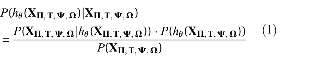
where θ are the synaptic parameters (or simply neural network weights) that have to be optimized, h_θ is the hypothesis of damage state (i.e. existence, location, size, and type of damage) which is dependent on the captured signal X_Π,_T,Ψ,Ω, and influenced by parameter tuples Π, T, Ψ, Ω, which correspond to actor, transitional, medium, and environmental domain, respectively. A detailed explanation of these parameters can be found in Ewald et al., ²⁵ and to summarize we depict the above-mentioned parameters in Figure 1. Equation (1) can be understood by considering that the posterior belief P(h_θ(X_Π,_T,Ψ,Ω)|X_Π,_T,Ψ,Ω) is equal to the multiplication of the prior belief P(X_Π,_T,Ψ,Ω) by the likelihood P(X_Π,_T,Ψ,Ω|h_θ(X_Π,_T,Ψ,Ω)) that X_Π,_T,Ψ,Ω will occur given that h_θ is true. Typically, for SHM (but also for NDT) the objective is to maximize the value of P(h_θ(X_Π,_T,Ψ,Ω)|X_Π,_T,Ψ,Ω) which means it should be close to, if not equal, to 1. This objective can be formulated mathematically as either a sigmoid function or with the generalized logistic regression (also called softmax) ²⁸ which maps any real values from ℝ into the range [0, 1].

Figure 1.

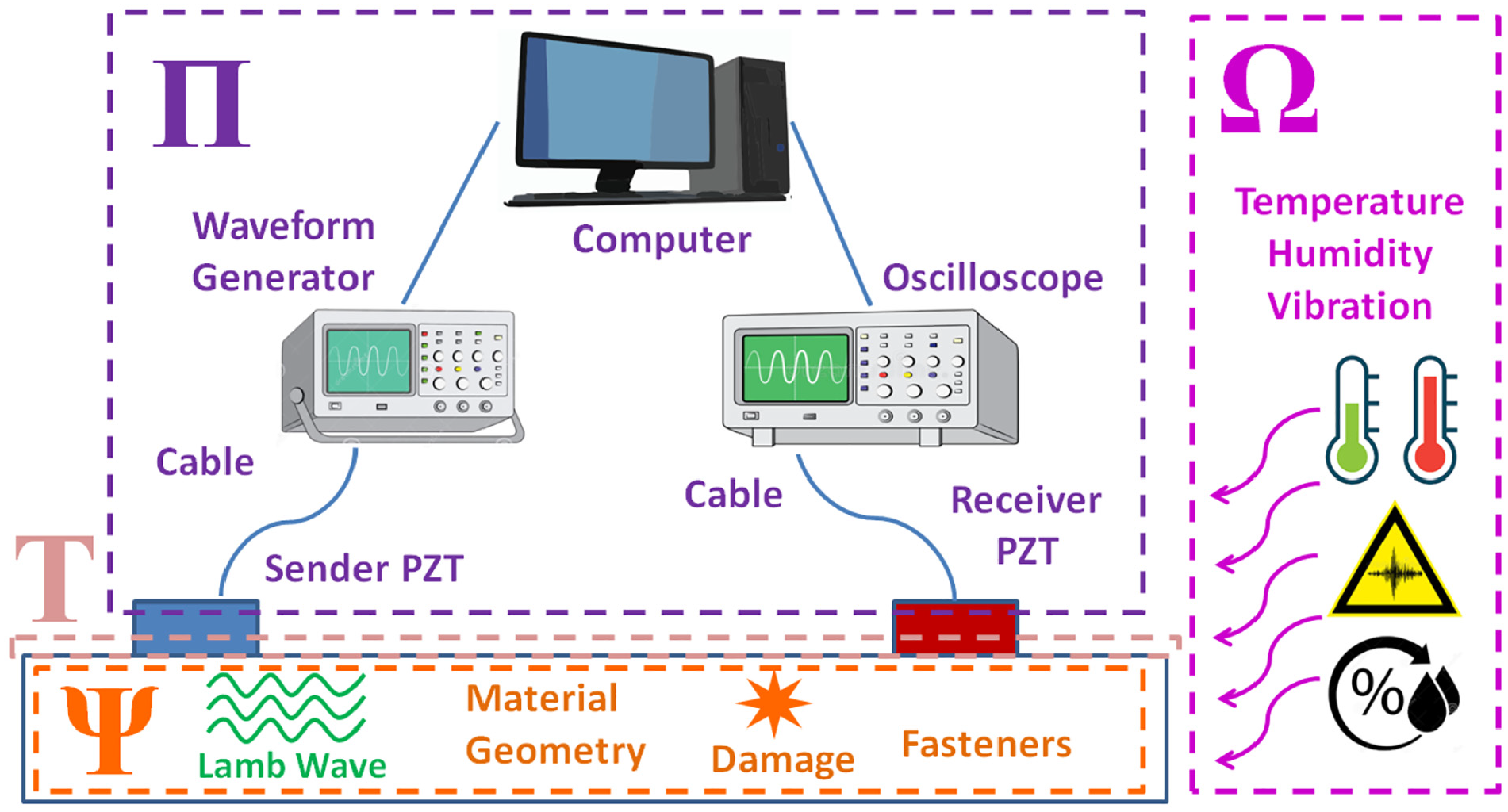
The realm of ultrasonic Lamb wave SHM with piezoelectric transducer (PZT), where Π, T, Ψ, Ω are actor, transitional, medium, and environmental domain, respectively.

Assume that the observed signal X_Π,_T,Ψ,Ω consists of k-features, then the predicted probability for the jth class of damage information given the signal X_Π,_T,Ψ,Ω given k-dimensional Hilbert space is

$$P(h_{\theta }({\mathbf{X}}_{\mathbf{\Pi },\mathbf{T},\mathbf{\Psi },\mathbf{\Omega }})=j|{\mathbf{X}}_{\mathbf{\Pi },\mathbf{T},\mathbf{\Psi },\mathbf{\Omega }})=\frac{\exp ({[{\mathbf{X}}_{\mathbf{\Pi },\mathbf{T},\mathbf{\Psi },\mathbf{\Omega }}]}^T·{\theta }_j)}{\sum _{k=1}^K\exp ({[{\mathbf{X}}_{\mathbf{\Pi },\mathbf{T},\mathbf{\Psi },\mathbf{\Omega }}]}^T·{\theta }_k)}$$

(2)

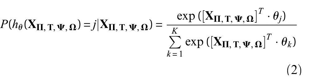
All machine learning models involve a training algorithm to obtain the optimal model parameters θ. Once the training is done, the model is tested to judge its prediction reliability. For both SHM and NDT, the objective is to maximize the true positives (TPs) and to minimize false negatives (FNs), thus maximizing the POD, also known as the sensitivity or recall rate in the confusion matrix

$$\mathrm{POD}=\frac{\sum \mathrm{TP}}{\sum (\mathrm{TP}+\mathrm{FN})}$$

(3)

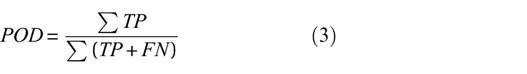
In equation (3), TP and FN can only take Boolean values B as defined in

$$B=\{\begin{array}{cc}1\hfill & \begin{array}{cc}\mathrm{if}\hfill & \mathrm{sgn}(max(P(h_{\theta }({\mathbf{X}}_{\mathbf{\Pi },\mathbf{T},\mathbf{\Psi },\mathbf{\Omega }})=j|{\mathbf{X}}_{\mathbf{\Pi },\mathbf{T},\mathbf{\Psi },\mathbf{\Omega }})\hfill \end{array}))=1\hfill \\ \multicolumn{1}{c}{0}& \begin{array}{c}\begin{array}{c}\mathrm{else}\hfill \end{array}\hfill \end{array}\hfill \end{array}$$

(4)

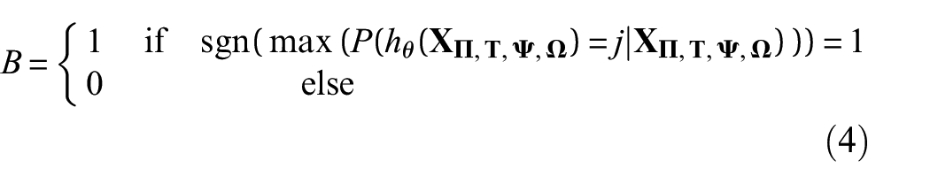
which means that the posterior belief P(h_θ(X_Π,Ψ,Ω) = j|X_Π,Ψ,Ω) takes value 1 if its maximum probability is signed as 1. The general objective of SHM is then given by

$$\begin{array}{c}\underset{\mathbf{\theta },\mathbf{\Pi },\mathbf{T},\mathbf{\Psi },\mathbf{\Omega }}{\arg \max }P(h_{\theta }({\mathbf{X}}_{\mathbf{\Pi },\mathbf{T},\mathbf{\Psi },\mathbf{\Omega }})=j|{\mathbf{X}}_{\mathbf{\Pi },\mathbf{T},\mathbf{\Psi },\mathbf{\Omega }})\hfill \\ \Rightarrow \underset{\mathbf{\theta },\mathbf{\Pi },\mathbf{T},\mathbf{\Psi },\mathbf{\Omega }}{\arg \max }\mathrm{TP}\hfill \end{array}$$

(5)

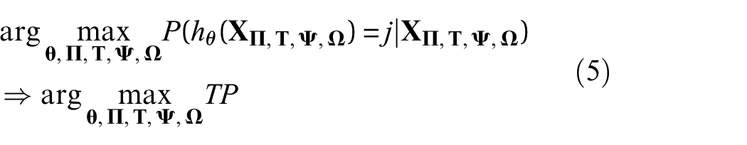
From equation (5), it can be seen that there are a manifold of parameters in Π, T, Ψ, Ω that can be fine-tuned, but one of the crucial parameters that influences the posterior belief is the sensor coordinate, ²⁶ which is contained in the actor domain Π because not all locations in the material will receive the same energy. A more detailed derivation on amplitude calculation at any arbitrary point in the material can be found in Bao ²⁹ and Su and Ye. ³⁰ As the piezoelectric transducers (PZTs) are permanently attached to the structure, it might pose a problem if the sensor network topology can only detect a locally propagating Lamb wave. In that case, P(h_θ|X_Π,_T,Ψ,Ω) will be per se lower and the overall SHM system reliability would be low.

Search metaheuristics

As there are many possibilities to position the sensors, it is not viable to test every single sensor network configuration. This will be explained in detail in section “Sensor positioning for detection of random damage occurrences.” When an exhaustive brute force search takes too much time, normally a heuristic search is employed to find a close-to-optimal solution within a reasonable amount of time. To find a viable solution from such a large search space, one could consider the following approaches: (1) no prior knowledge was used during the decision-making; thus, the decision probability is equally distributed over the decision set, (2) prior knowledge is used in the decision-making and for sorting the decision options, and (3) no prior knowledge was involved at the beginning but is gradually incorporated as the decision-making process evolves.

These approaches can be related to several popular search heuristics.^31–34 In a random search, ³¹ no prior knowledge is required. For the greedy algorithm, ³² the prior knowledge is required to sort available decision options. In GA,^33,34 no prior knowledge is required at the beginning, but decision options are updated after including this information. These approaches to sensor positioning are briefly described in sections “Global random search” to “GA.”

Global random search

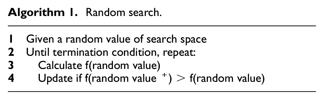
Global random search is the easiest method to use to solve combinatorial problem. However, given a limited time constraint, it is also the least efficient since the optimal sensor position might not be found. The algorithm is very simple and can be demonstrated in only four lines of pseudocode, as shown in Algorithm 1. The random value in this case is a random position of x_i, y_j.

Algorithm 1.

Random search.

1 Given a random value of search space 2 Until termination condition, repeat: 3  Calculate f(random value) 4  Update if f(random value +) > f(random value)

Greedy algorithm

According to Cormen et al., ³² “a greedy algorithm always makes the choice that looks best at the moment. That is, it makes a locally optimal choice in the hope that this choice will lead to a globally optimal solution.” For some problems, the greedy algorithm can provide an optimal solution, while in other cases it does not, ³² because sometimes the selected solutions reach a local optimum. In many cases, a greedy algorithm is designed as a sequential process, but it is possible also divide the search spaces and assign a greedy agent to each particular search space and to execute each task in parallel. For brevity, the example pseudocode of a sequential greedy algorithm is shown in Algorithm 2.

Algorithm 2.

Greedy algorithm.

1 Given a set of particular value of search space 2 Until termination condition, repeat: 3  Calculate f(value) 4  Sort f(value) from min to max 5  argmax f(value)

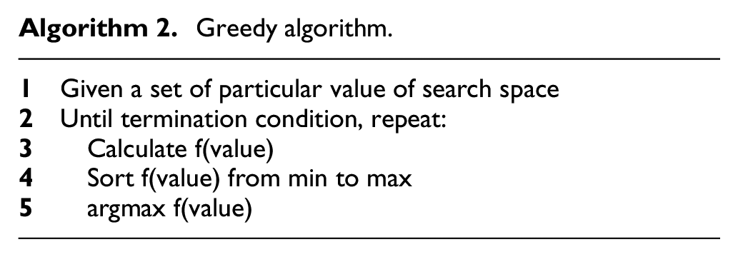
In the greedy algorithm, the function value will be sorted from the minimum to maximum, and the argument maximum is chosen as the optimal solution. For multiple sensors, the greedy algorithm will search the next optimal sensor position step by step. That is, the next sensor position is determined by the previous sensor position by considering the last previous sensor position. In practice, this will lead to locally optimal solutions that might still be globally optimal solution within reasonable amount of time.

GA

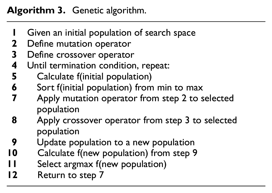
The GA is a biologically inspired algorithm from the Darwinian concept of natural evolution. ³³ More concretely, it is a metaheuristic search approach that is applicable to many optimization problems. Usually, a GA contains three main operators: mutation, crossover, and selection. ³⁴ Typically, the procedure starts with a given initial population that will be assessed against its fitness. Those individuals that have the best fitness are crossed-over with each other and/or a “genetic mutation” is applied, for example, by bit-flipping or replacement. The individuals who do not have the best fitness are not selected. This procedure is repeated several times until a specified certain termination condition is reached. A typical GA is described in Algorithm 3.

Algorithm 3.

Genetic algorithm.

1 Given an initial population of search space  2 Define mutation operator  3 Define crossover operator  4 Until termination condition, repeat:  5  Calculate f(initial population)  6  Sort f(initial population) from min to max  7  Apply mutation operator from step 2 to selected population  8  Apply crossover operator from step 3 to selected population  9  Update population to a new population 10  Calculate f(new population) from step 9 11  Select argmax f(new population) 12  Return to step 7

For the sensor placement problem, the sensor coordinates x_i, y_j are first encoded as a chromosome (Figure 2) that will be assessed against the fitness function in line 10 of Algorithm 3. The genome length is 2N, where N is the amount of the sensors to be installed.

Figure 2.

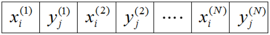
Sensor position as chromosome in genetic algorithm for N sensors.

Typically, the aircraft manufacturer or operator will determine how many sensors are to be installed based on the balance between cost, additional weight, POD/sensor network performance and safety. Generally, more sensors installed means a higher Lamb wave coverage, but this also means higher costs and energy consumption, and more weight since every sensor is attached to a cable. Also, after a certain number of sensors, the coverage will only slowly increase up to the upper limit of the sensor network performance.

As defined in Algorithm 3, there are two basic operations in a GA: the mutation and the crossover operator. The mutation operator alters one or more values in the chromosome and its purpose is to preserve and introduce diversity, while the crossover operator is used to combine the genetic information of two parents to generate new children. In practice, there are many other ways to conduct mutations and genetic operations.^33,34 For a simplified illustration, we will only show the most common methods in Figure 3.

Figure 3.

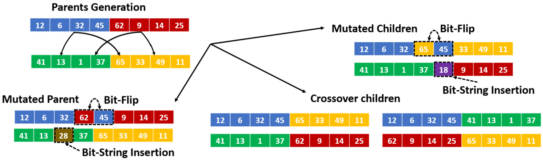
Basic operation of genetic algorithm: mutated and crossover from parent generation.

In a single-point crossover, the parent chromosome is divided into two sub-genomes and the genome information is permuted in order to derive the crossover children. To create a mutated generation that can be either a mutated parent or a mutated child, two common methods are normally used: (1) the bit string mutation (where a random chromosome is inserted into individual) and (2) the bit-flip mutation (where the chromosome order in the mutated individual is flipped). The mutation operation rate is required to be larger than 0 to avoid being stuck in a local minima, but is typically kept low, so that the algorithm does not jump too fast from one optimum to another optimum as both of these conditions make the search unnecessary long.

Methodology

In our previous work, ²⁴ we demonstrated a method to optimize the transducer placement for Lamb wave–based SHM for detection of a fatigue crack that emerges from a rivet hole in an aircraft fuselage panel. In this article, we focus on barely visible impact damage that is typically caused by low velocity impact (LVI) which is defined as under 50 m/s. ³⁵ If we design an SHM system to detect this impact damage according to the deterministic approach, then the sensor configuration would change for each possible impact location, hence rendering the deterministic approach useless because it would require millions, if not more experimental validations.

In mathematics and computer science, a comparable problem to this sensor network coverage optimization is called the Art Gallery Problem, which originates from a real-world problem of guarding an art gallery with the minimum number of guards who together can observe the whole gallery. ³⁶ Conceptualizing the art gallery problem into SHM sensor positioning design means we would like to maximize the coverage of the monitored area given a minimum number of PZT sensors. The design of an SHM system to detect random damage locations in an aircraft is a combinatorial problem of similar complexity, where it is often assigned as NP-complete where NP stands for non-deterministic polynomial time, which means that such problems are solvable in polynomial time on a non-deterministic Turing machine. ³⁷

Sensor positioning for detection of random damage occurrences

As previously explained, the deterministic approach would require too many simulations, and is computationally unfeasible. Thus, it would be useful to maximize the sensor coverage area to detect damages that occur within that coverage area. Therefore, we create a target function that describes the attenuation at a certain location in the propagation space of the Lamb wave. First, consider the measured signal power P in an infinite plate at point x where the original excitation signal power is P₀,^39,42 the geometrical attenuation factor α is proportional to 1/√r^30,38–41 and r is the distance from the wavefront to the point x

$$P=P_0·\alpha ·\exp (-\beta ·r)\begin{array}{cc}\mathrm{where}\hfill & \alpha \hfill \end{array}\propto \frac{1}{\sqrt{r}}$$

(6)

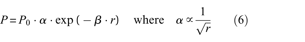
The material attenuation β depends on frequency and thickness, for example, for a 1-mm thick aluminum plate, the attenuation coefficient is between 2.2 and 17 dB/m for a frequency between 0.5 and 5 MHz.^39,42 For a given coordinate (x_i, y_j), we can construct an effective travel distance assigned in pixel value f(r_ij) by multiplying the total attenuation [α_ij·exp(−β·r_ij)] by the propagating distance r_ij from the wave propagation source so that it is comparable to a measured Lamb wave signal amplitude attenuation profile

$$f(r_{\mathrm{ij}})=r_{\mathrm{ij}}·[{\alpha }_{\mathrm{ij}}·\exp (-\beta ·r_{\mathrm{ij}})]\begin{array}{cc}\mathrm{where}\hfill & {\alpha }_{\mathrm{ij}}\propto \frac{1}{\sqrt{r_{\mathrm{ij}}}}\hfill \end{array}$$

(7)

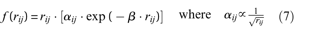
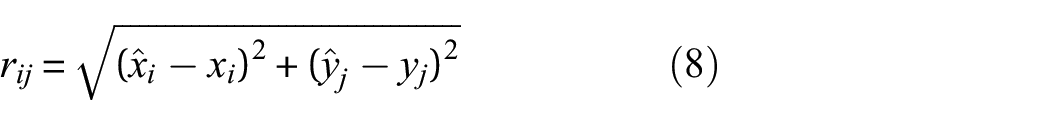
where the distance r_ij is defined as the Euclidian distance from the wave propagation source at coordinate (x_i, y_j) up to an arbitrary pixel located in coordinate (◯_i, ŷ_j) and α_ij is the dimensionless geometric spreading correction factor at the distance r_ij

$$r_{\mathrm{ij}}=\sqrt{{({\hat{x}}_i-x_i)}^2+{({\hat{y}}_j-y_j)}^2}$$

(8)

Consider a structural inhomogeneity such as rivet hole at a coordinate ( ${\tilde{x}}_i,{\tilde{y}}_j$ ) that acts as a secondary source, since a Lamb wave wavefront is scattered at the rivet holes. In our assumption, we simplified the scattering occurring at the rivet to be homogeneous in all direction. While this is not very realistic, the scatter from such small rivets tends to be small in amplitude.^43–45 A more detailed analytical scattering model could be included in the calculation if a reliable formula is available. Regardless of the scattering direction, the secondary source emits a lower energy as the waves have lost energy in traveling from the source PZT to the rivet hole via the indirect path $\mathrm{tilde}{r}_{\mathrm{ij}}$ defined by

$$\begin{array}{c}\multicolumn{1}{c}{{\tilde{r}}_{\mathrm{ij}}=r_{\mathrm{PZT}-\mathrm{rivet}}+r_{\mathrm{rivet}-\mathrm{pixel}}=\sqrt{{({\tilde{x}}_i-x_i)}^2+{({\tilde{y}}_j-y_j)}^2}}\\ +\sqrt{{({\tilde{x}}_i-{\hat{x}}_i)}^2+{({\tilde{y}}_j-{\hat{y}}_j)}^2}\hfill \end{array}$$

(9)

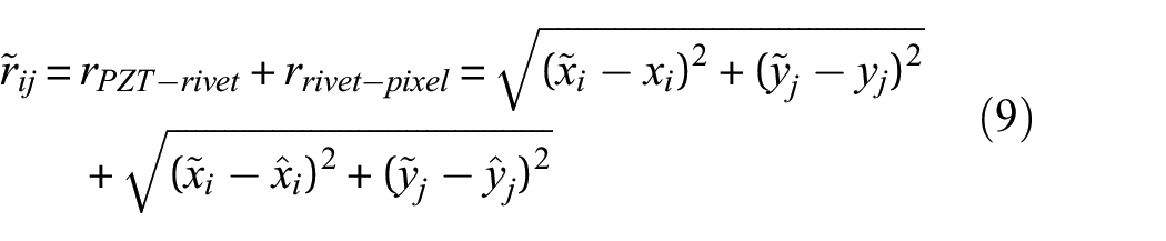
The pixel value in equation (7) for the secondary source can be rewritten in equation (10)

$$\begin{array}{c}\multicolumn{1}{c}{f({\tilde{r}}_{\mathrm{ij}})=r_{\mathrm{rivet}-\mathrm{pixel}}·[{\tilde{\alpha }}_{\mathrm{ij}}·\exp (-\beta ·{\tilde{r}}_{\mathrm{ij}})]}\\ =r_{\mathrm{rivet}-\mathrm{pixel}}·[\frac{1}{\sqrt{r_{\mathrm{PZT}-\mathrm{rivet}}·r_{\mathrm{rivet}-\mathrm{pixel}}}}·\exp (-\beta ·{\tilde{r}}_{\mathrm{ij}})]\hfill \end{array}$$

(10)

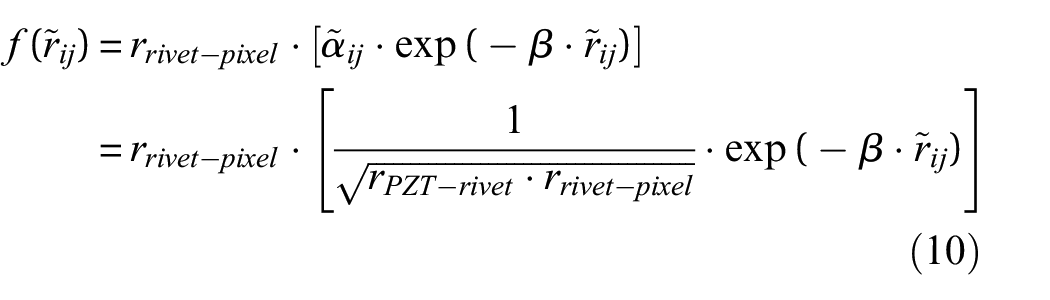
where ã_ij is the recalculated geometrical spreading correction factor at distance r_ij. As an example, consider a resolution of 1 pixel that corresponds to 1 cm in reality. The function values of equations (7) and (10) for different values of β with the distance r_rivet-pixel = 0.25 m are depicted in Figure 4(a) and (b), respectively. Note that this pixel value is only a dimensionless construct to indicate the Lamb wave attenuation profile. The intuition that leads to the above-mentioned fitness function is that it would be favorable for the Lamb wave to travel as far as possible; however, this is limited by the attenuation. Damage that happens in the area which is too close to the wave source would probably have a lower POD and an impact that happens in the area which is too far from the wave source would also likely to have lower POD. The sweetspot would be then in between, as shown in Figure 4(a) and (b).

Figure 4.

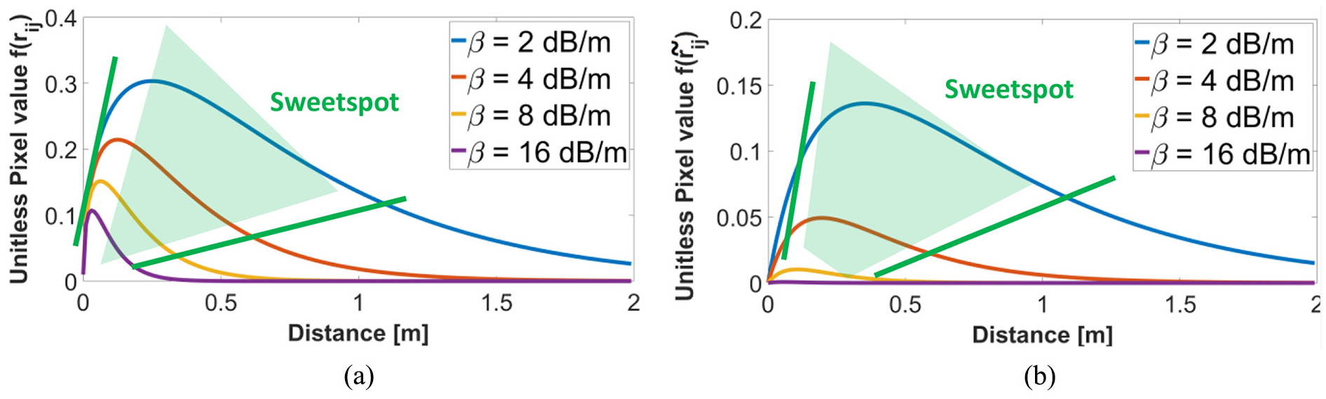
Unitless pixel value of (a) f(r_ij) and (b) f( ${\tilde{r}}_{\mathrm{ij}}$ ) as a function of distance which is comparable to amplitude profile. For demonstration purpose, the curve in Figure 4(b) is calculated based on ${\tilde{r}}_{\mathrm{ij}}$  = 0.25 m + r_rivet-pixel.

We constructed the pixel value not only based on the attenuation profile (which goes toward +∞ very close to the source) but also to anticipate the near-field zone (NFZ), known as the dead zone since where it is difficult to evaluate any flaws. For simplicity, we only consider the NFZ to be the area which is covered directly by the PZT.

Lamb wave scattering occurs repeatedly, but each consecutive scattering event reduces the energy. Depending on the modes, material, excitation frequency, and thickness, the attenuation β can vary between 0.001 and 0.005 dB/cm. ⁴⁶ For instance, in carbon fiber reinforced polymer (CFRP) woven (10-ply), the A₀-mode Lamb wave excited at 285 kHz would only need to travel 85 mm until 90% decay. ³⁰ In woven CFRP of 8-ply, the S₀-mode Lamb wave excited at 250 kHz would need to travel 1700 mm until the 90% decay. ³⁰ Generally, the S₀-mode tends to travel further than the A₀-mode due to the fact that the A₀-mode Lamb wave is dominated by perpendicular displacement relative to the wave propagation direction; thus, it is leaking more energy to the surrounding environment. ³⁰

In contrast, the S₀-mode is dominated by the in-plane particle displacement, so that energy is better conserved within the plate, as the partial energy leakage is lesser than the A₀-mode. For the consecutive scattering, Su and Ye ³⁰ suggested to compensate the energy loss due to geometrical spreading for by multiplying the measured signal magnitude with the square root of the time elapsed as given by

$$\hat{f}(t)=f(t)·\sqrt{t}$$

(11)

Consider the example proposed by Zhao et al., ⁴⁷ where transducer T is placed between rivet holes as depicted in Figure 5(a) (Case 1). Given that actuator T was excited using a 1.8-MHz excitation frequency, Figure 5(b) illustrates the captured S₀-mode Lamb wave signal from a series of sensors X that are located 20–200 mm away from the actuator T. In this case, they calculated that the average attenuation rate was 0.044 dB/mm. In Case 2, they placed sensor series Δ across the stiffeners, and using the same frequency and S₀-mode excitation obtained an average attenuation of 15 dB per rivet row. The distance between the rivet rows was 6.5 cm, meaning that the average attenuation was increased to 0.231 dB/mm. This calculation already included the multiple scattering across the rivets.

Figure 5.

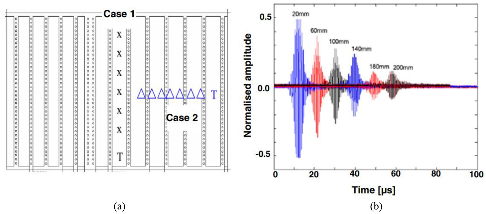
(a) Sketch of distribution of rivets and transducers in wing section (“T”: actuator; “X”: sensor in Case 1; “Δ”: sensor in Case 2); and (b) integrated Lamb wave signals captured by a series of sensors in a straight line (Case 1). ⁴⁷

For brevity, we consider the first appearance of the wave scattering until the wave is absorbed at the boundaries of the plate. The calculated pixel score s_ij at pixel ( ${\tilde{x}}_i,{\tilde{y}}_j$ ) for a given N transducers and B inhomogeneities can simply be defined as a summation of normalized function values f(r_ij) and $f{\tilde{r}}_{\mathrm{ij}}$ )

$$s_{\mathrm{ij}}=\sum _N||f(r_{\mathrm{ij}})||+\sum _B||f({\tilde{r}}_{\mathrm{ij}})||$$

(12)

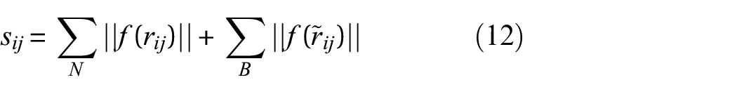
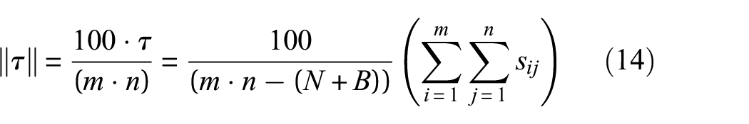
The network fitness score τ is simply the summation of all pixel scores, excluding the pixel P ϵ P_N or P_B, which are occupied by the transducers N and inhomogeneities B, respectively

$$\begin{array}{c}\multicolumn{1}{c}{\tau =\sum _{i=1}^m\sum _{j=1}^n{s}_{\mathrm{ij}}}\\ \multicolumn{1}{c}{\mathrm{where}{s}_{\mathrm{ij}}=0\mathrm{if}P\in P_N(x_i,y_j)\vee P_B(\widetilde{x_i},\widetilde{y_j})}\end{array}$$

(13)

As previously stated, we currently consider the approximated effective NFZ to be the area directly below the PZT. The rivet hole is idealized as a “secondary actuator,” with the simplification that the wave scatter from the rivet hole is homogenously reflected to all directions, although in practice, it depends on the direction of the coming wavefront. Thus, it is logical to set the pixel score to be 0 at those occupied pixels as they do not act as wave detection points. In addition, equation (13) can be normalized to take any positive real number between 0 and 100

$$||\tau ||=\frac{100·\tau }{(m·n)}=\frac{100}{(m·n-(N+B))}\left(\sum _{i=1}^m\sum _{j=1}^n{s}_{\mathrm{ij}}\right)$$

(14)

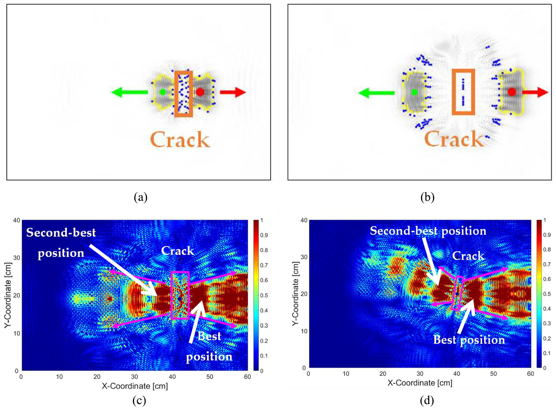
Examples of the network score mapping for transducers placed at coordinates 40|40 cm and 115|10 cm in a plate with dimension of 120 × 80 cm are given in Figure 6(a) and (b), respectively, while their alternative representations in three-dimensional (3D) projection are depicted in Figure 6(c) and (d), respectively. In Figure 6(a) and (b), the sensor and rivet hole locations are red dots in locations indicated by white and black rectangles, respectively. Figure 6(a) shows that the whole plate is better covered if the PZT is located at 20|40 cm since the network score is 39.73. In comparison in Figure 6(b) (PZT location at 115|10 cm), the network score is only 33.17. Our definition of coverage is any pixel location where a direct or scattered wave propagates. Thus, a network score of 39.73 can be considered as the average wave amplitude is 39.73% of the maximum. Note that until equation (14), we consider neither the signal processing parameters nor the algorithm yet (except the anticipation toward the NFZ). The value of coverage level can be later adjusted once the thresholding parameter has been determined.

Figure 6.

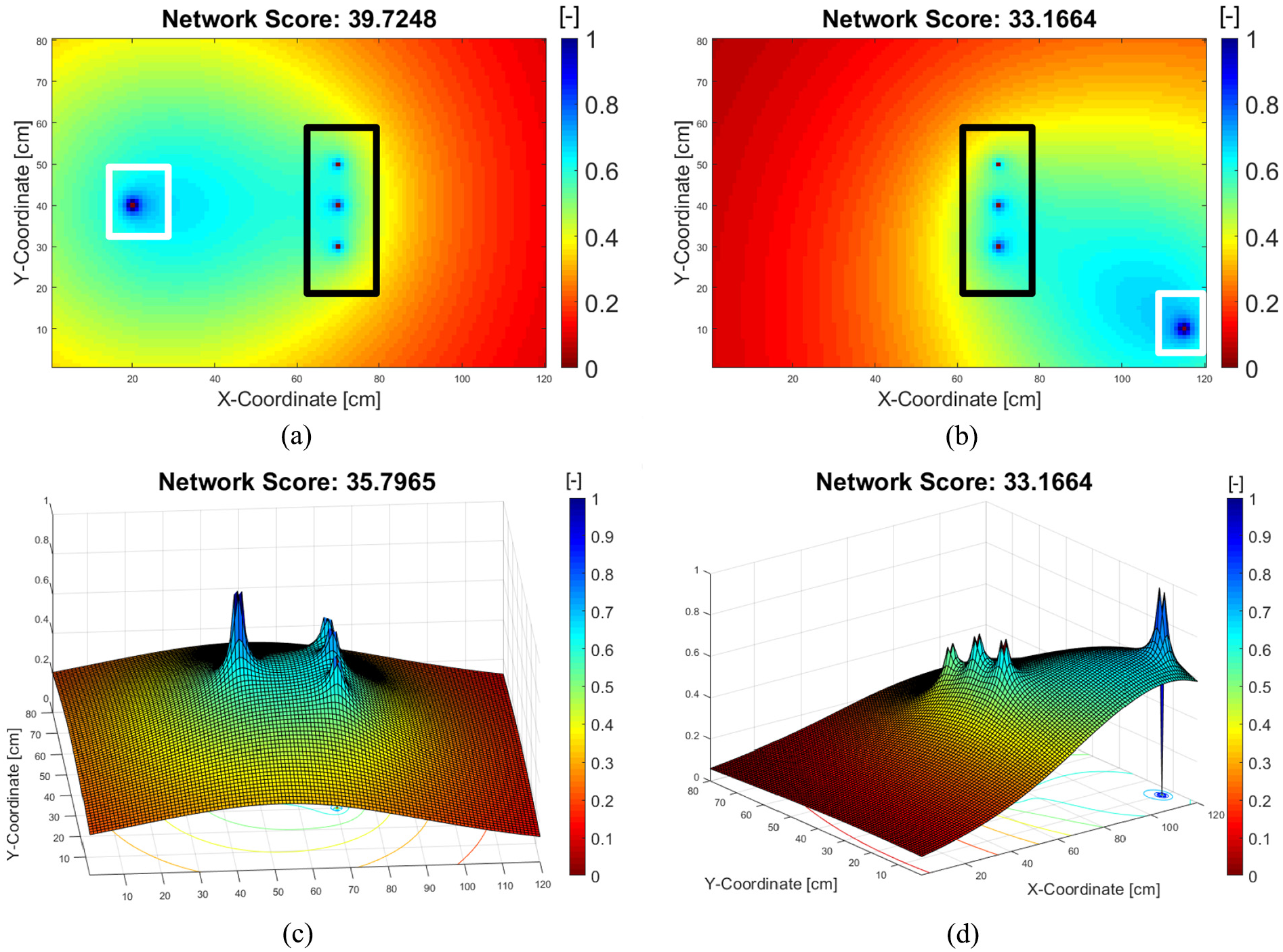
Mapped unitless pixel score s_ij and network score τ for transducer placement at (a) 20|40 cm and (b) 115|10 cm. Figure (c) and (d) are the alternative representations of the network score in three-dimensional projection. The white and black rectangles signify the sensor and rivet hole locations, respectively.

Furthermore, the network score will decrease, if the attenuation coefficient β is increased as depicted in Figure 7 (cf. with Figure 6(a) that has an attenuation coefficient β = 0.3). The attenuation coefficient depends on the material properties and excitation frequency.^39,42 This implies that even if the material is the same, the network score will be lower if a higher excitation frequency is applied.

Figure 7.

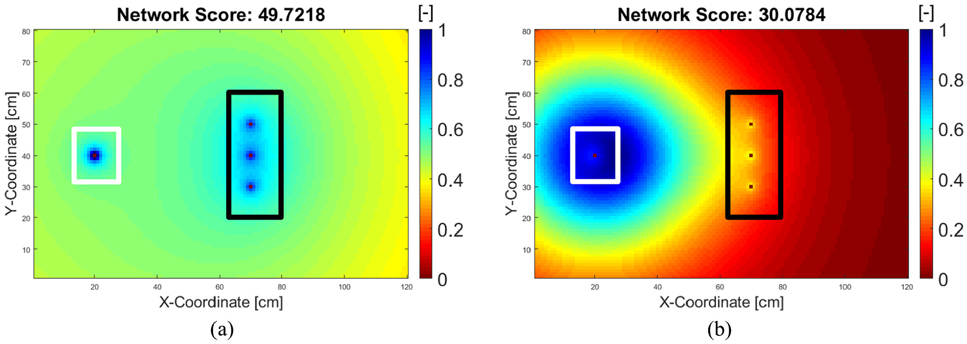
Mapped pixel score s_ij and network score τ for transducer placement at 20|40 cm for (a) β = 0.1 and (b) β = 0.7. The white and black rectangles signify the sensor and rivet hole locations, respectively.

The maximum network score is reached at ||τ|| = 100; thus, the objective is defined as

$$\underset{{(x_i,y_j)}^{(N)}}{\arg \max }(||\tau ||)$$

(15)

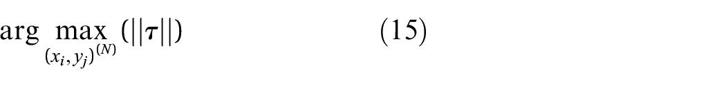
Equation (15) reads, given N number of sensors, determine the coordinate (x_i, y_j) of each actuator N that maximizes the network fitness score τ. Theoretically, the maximum value is the total amount of pixels without (N + B) as per equation (13). For example, a plate with a size of 120 × 80 cm and 2 mounted sensors and 3 rivet holes would have a theoretical maximum score of 9600 − (2 + 3) = 9595, or 99.9479 if it is normalized using equation (14).

The physical interpretation of equation (15) means that at the maximum network score, a minimum attenuation is reached. Assuming that the PZT sensors can capture any wave scatter due to the damage occurring at anywhere on the plate and coupled to adequate signal processing, the sensor network will be able to detect and predict the damage location reliably.

From equations (12) to (15), it is obvious that the network fitness score is independent of the DI. This at least eases the transducer placement search for the best fitness. However, to search for the best fitness, it would still take a lot of time even without determining the DI from experiment. The number of possible sensor placement combinations C of given N sensors, B inhomogeneities, and L pixels is given by equation (16)

$$C=\frac{(L-B)!}{N!(L-B-N)!}$$

(16)

As an example, assume each pixel size is 1 × 1 cm, then for a plate of 120 × 80 cm for a single sensor (N = 1) and 3 rivet holes (B = 3) in which there are C = 9597 possible combinations, the computation time for the brute force search with our PC specification in 2.57 s. However, for two, three, and four sensors, the calculation time would increase from 3.4 h to 15 months and to 3000 years, respectively.

Integrative approach

As previously explained, hotspot SHM design has the job of monitoring damage that can already be predicted during the design phase. On the contrary, the probabilistic approach for SHM described in sections “Search metaheuristics” and “Sensor positioning for detection of random damage occurrences” is only useful for detecting random damage locations. Our proposed SHM system design is to integrate both approaches in one. This is because when aircrafts are in service, they are prone to both types of damages whose occurrences are likely to be independent of each other. For instance, a fatigue crack might grow from one rivet hole depicted in Figure 5(a), while the area in between the rivet rows could be prone to a tool drop or hail impact.

Assuming that this scenario is likely to happen, we highly doubt that there is a strong likelihood that the fatigue crack growth will suddenly induce the probability of hail impact or tool drop occurrence between the rivet rows. However, a hail impact could induce fatigue crack growth. Thus, such a multiple damage location probability with independent nature, the novel approach we are proposing here is first to give the priority to hotspot SHM sensor locations and then to determine the additional sensor locations for detecting random damage, starting by reusing the hotspot sensor locations.

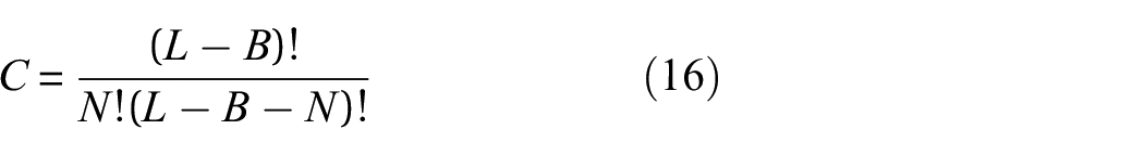
That is, we took the best two positions (this number can be adjusted according to Original equipment manufacturer (OEM) or aircraft operator requirement) from the hotspot SHM design and then conducted the metaheuristics methods to search for the additional suitable locations. We propose that the two hotspot SHM sensors can also be used to detect Lamb wave scatter which originates from random damage. To determine the hotspot sensors’ locations, a blob detection and fused images of the wave propagation was used, as depicted in Figure 8. ²¹

Figure 8.

Detected blobs during wave propagation (red and green arrows signify the propagation direction of the wave scatter) at (a) 100 µs and (b) 125 µs. Fused differential images to obtain the best sensor positions for (c) 60-mm hotspot perpendicular crack and (d) 60-mm hotspot crack with 8° orientation. ²¹

Results

Global random search

The results of the global random sensor position (see section “Global random search”) search are depicted in Figure 9(a) and (b). Figure 9(a) depicts an example result of a search for three sensors, while Figure 9(b) depicts the result of a search of six sensors. While the result would normally change for each iteration, it is possible for the random search to converge with an increasing number of sensors (see Figure 10). Figure 10 depicts the average network score after 10 searches for 1–10 sensors search from 1 to 1000 iterations.

Figure 9.

Random search for (a) three sensors and (b) six sensors with black and white rectangles convention from Figures 5 and 6.

Figure 10.

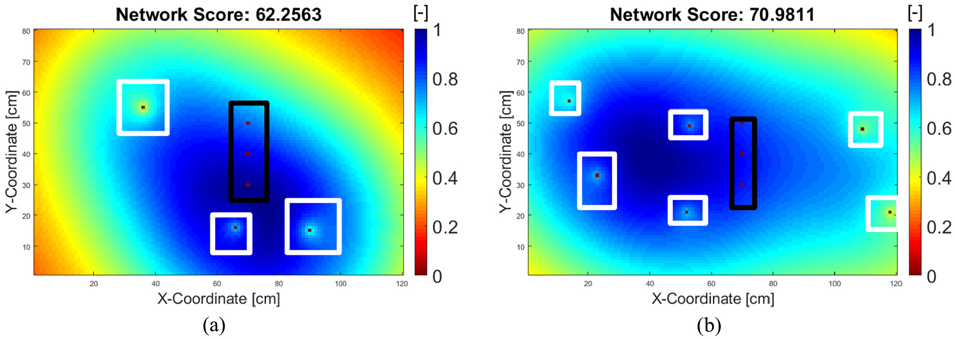
Distribution of network score for random search algorithm of 1–50 sensors after 1000 iterations. Error bars indicate the standard deviation of the network score during 1000 iterations.

As one can see in Figure 10, the random search algorithm starts to converge from five sensors, with decreasing standard deviation (indicated by the error bars), toward an average network score of around 81, which means the plate is 81% covered by the wavefront should an impact happen anywhere on the plate. A similar convergence can also be observed in the work of Soman et al., ¹⁹ where they reached the convergence at eight sensors for a plate of 100 cm × 100 cm (ours is 120 cm × 80 cm). The computational time, as expected, is linear since the calculation effort is the same for every iteration—and in this case, the complexity notation is denoted as O ( n ).

Greedy algorithm

The mode of operation of the greedy algorithm is depicted in Figure 11(a) to (d). The algorithm first finds the optimum position of one sensor (Figure 11(a)), then calculates the next best sensor position based on the position of the previous sensor. As can be seen from Figure 9(a) versus Figure 11(b), the greedy algorithm for three sensors search (network score = 73.18) performs better than global random search (average network score = 68.15). This is expected because the random search does not have clear strategy to find the maximum except by saving the best possible solution for each iteration, while the strategy of finding the maximum in the greedy algorithm is by dividing the problem into smaller sub-problems.

Figure 11.

(a to d) Greedy search for 1, 3, 5, and 7 sensors, respectively. Black and white rectangles convention apply.

By replacing the first line in Algorithm 2 with all possible sensor positions instead of only random values, it is possible for the greedy algorithm to determine the maximum theoretical network value thanks to the sorting function (line 4 in Algorithm 2), which in this case is 40.8884 as can be seen in Figure 10(a). The problem with this approach is when more than one sensor search is applied, the required calculation time is comparable to 9600 ^N for a plate size of 120 × 80 cm, where N is the amount of the sensors. Sorting is therefore not always feasible for a multivariable search.

GA

For the GA, we use the default MATLAB GA parameters that are specified in the GA optimization toolbox. Constraints such as only integer due discretization or the candidates must be fit within the plate dimension were specified in the MATLAB toolbox: population size is 50 candidates for less than 5 variables (2 sensors), or 200 candidates for more than 5 variables (>2 sensors). The default selection criteria are stochastic uniform with 5% elite population, and a crossover fraction set at 0.8. The mutation is uniformly distributed over candidates and for simplicity, only single-point crossover is applied. The default stopping criteria specified in MATLAB toolbox is when it reaches 100*(number of sensors)th generation or 50 stall generations without any time or fitness value limit.

The results from a GA for 1–8 sensor searches are depicted in Figure 12(a) to (f), respectively. From these figures, one can clearly see that the GA tends to outperform the global random search and greedy algorithms. For instance, for three sensor searches, the GA reaches a network score of 84.12 (Figure 12(c)) after 21 s, while the greedy algorithm only reaches a network score of 72.28 (Figure 11(b)).

Figure 12.

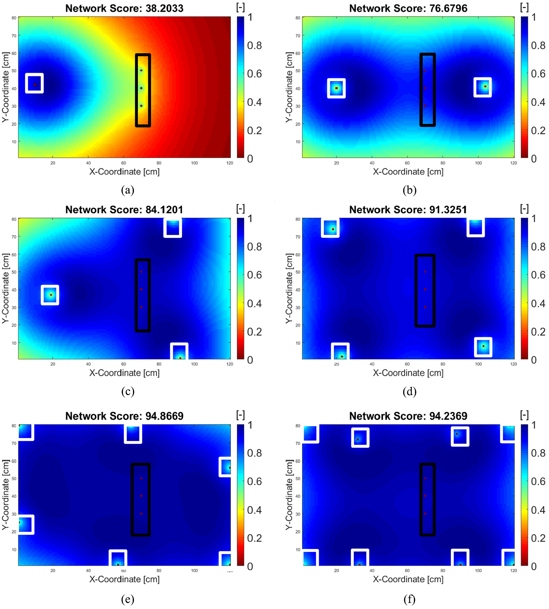
(a to f) Genetic algorithm search result for 1, 2, 3, 4, 6, 8 sensors. Black and white rectangles convention apply.

The random search performed even worse as it reaches a network score of 62.26 (Figure 9(a)). Note that for the special case of one sensor search, the GA was successful in finding the maximum theoretical value of the sorting greedy algorithm, which is 38.20 (cf. Figure 11(a) to 12(a))—thus, there is no difference in this case between the greedy and the GA, which proves that the construction of the GA worked in a consistent way.

However, it should be noted that the GA performs slowly, especially when the number of sensors increases, while the greedy algorithm and random search give a result almost immediately, a search with a GA for six sensors took almost 4 min. Not only that, the more sensors that are employed, the more computer memory is needed, sometimes forcing earlier termination of the algorithm and resulting a lower score, such as in Figure 12(f).

In a larger plate where more sensors are to be installed, a GA would deliver a high network score; however, this will be neutralized by its slower performance. To understand this more concretely, we must consider that all algorithms are bounded by time and space—thus, an algorithm performance is always related to the effort needed.

The implication would be that in such a larger plate, more sensors would be needed to increase the network coverage; thus, more computational effort is required to reach this level of performance. At some point however, the GA would also fail for higher number of sensors to run due to space limitation unless the computer memory is increased. That means, if we run the random search for hypothetically 3000 years instead of running the GA within 24 h for a given number of sensors, the random search would eventually reach the performance of GA without the complication of programming the genetic operators itself. This is actually in line with the No Free Lunch Theorem proposed by Wolpert and Macready ⁴⁸ :

Given a finite set V and a finite set S of real numbers, assume that f : V → S is chosen at random according to uniform distribution on the set S^V of all possible functions from V to S. For the problem of optimizing f over the set V, then no algorithm performs better than a blind search.

Preliminary conclusion

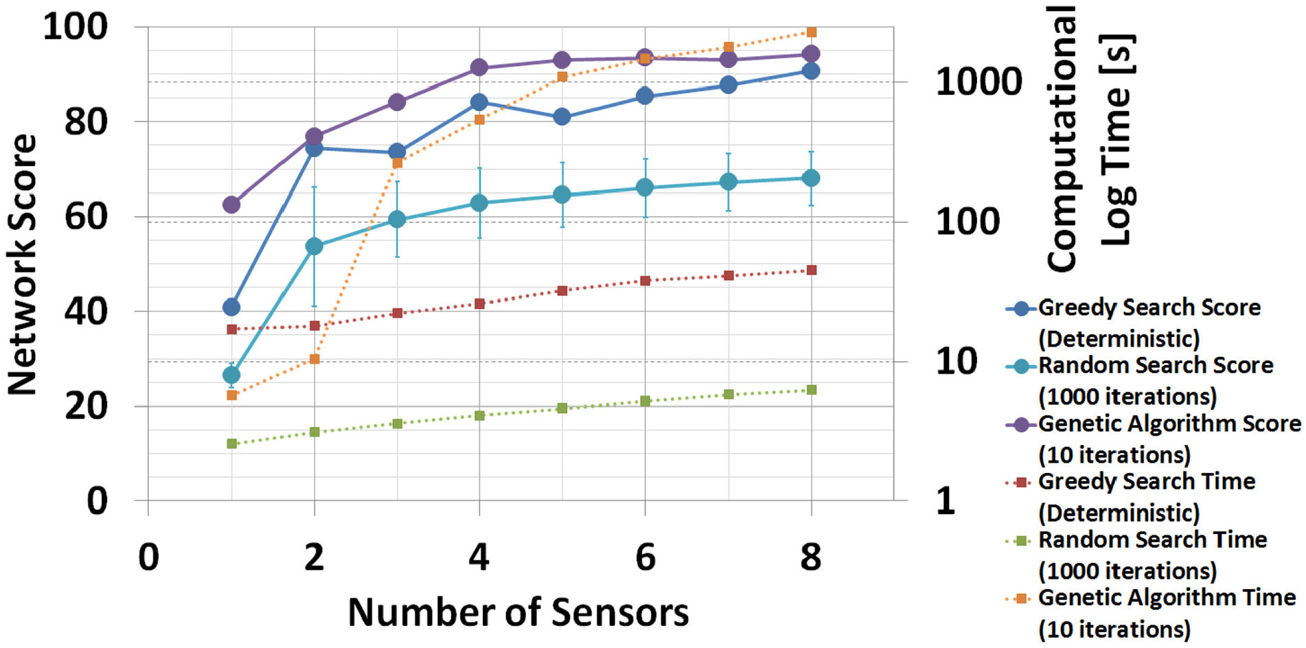
As a summary, a performance comparison of the global random search (after 1000 runs), greedy, and GAs (after 10 runs) is presented in Figure 12, where only the standard deviation σ from the random search is shown. Note that the standard deviation σ of the GA is too small to be visualized in the graph. The standard deviation of the greedy algorithm is 0. The X-axis represents the number of sensors, while the left Y-axis represents the network score reached by each algorithm. The right Y-axis represents the computational time needed for each algorithm.

Neglecting the computation time, it is obvious that the GA has the best performance from the three algorithms. However, taking the computation time into account, the greedy algorithm is competitive with the GA. Note that the right Y-axis has a logarithmic scale. Conversely, the random search took the lowest computational time while it has the lowest network performance.

It can be seen from Figure 13 that the GA starts to outperform the greedy algorithm from three sensors onwards; however, the 10-run GA took about 12 times longer (about 264 s) than the greedy algorithm. Also, note that in Figure 13, the standard deviation for the GAs cannot be shown as these are too small to be visualized (2.04 or less).

Figure 13.

Network score for random search algorithm of 1–8 sensors.

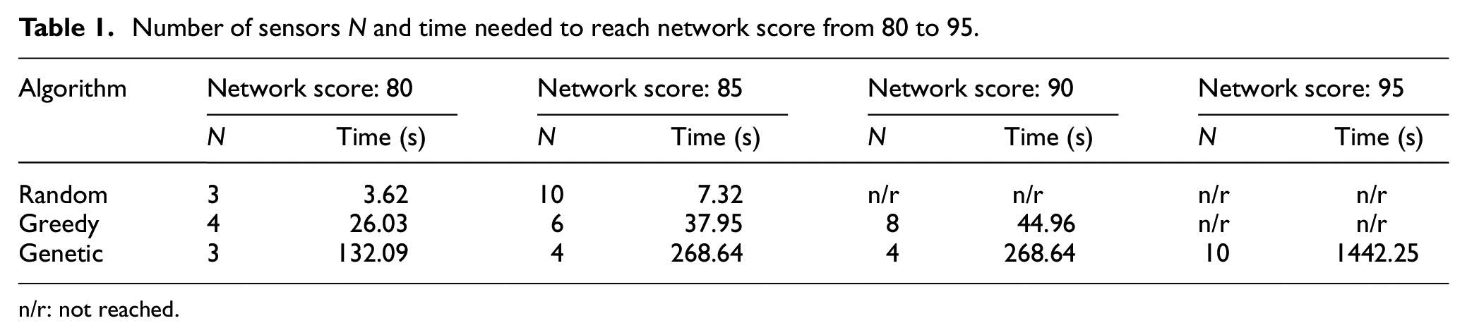
One could argue about the best terminating conditions of these algorithms. For this reason, we determined four different thresholds for the network score: 80, 85, 90, and 95 which can be understand as a coverage level between 80% and 95% of the surface—which when coupled with adequate signal processing, it can yield to global probability of damage detection POD of the network between 80% and 95%. We present the trade-off between the network score, number of sensors N, and the required computational time in Table 1. For brevity, we do not consider the hardware weights and the potential data redundancy as well as the system energy/power required as the number of sensors increases.

Table 1.

Number of sensors N and time needed to reach network score from 80 to 95.

Algorithm	Network score: 80		Network score: 85		Network score: 90		Network score: 95
	N	Time (s)	N	Time (s)	N	Time (s)	N	Time (s)
Random	3	3.62	10	7.32	n/r	n/r	n/r	n/r
Greedy	4	26.03	6	37.95	8	44.96	n/r	n/r
Genetic	3	132.09	4	268.64	4	268.64	10	1442.25

n/r: not reached.

As can be seen in Table 1, neglecting the required computational time, it is obvious that the GA has the best performance from the three algorithms, however, also requires the most computational time. Conversely, the random search has the lowest computational time while and the lowest network performance.

Integrated approach using blob detection and GA

The procedure described in Ewald et al. ²⁴ was repeated for an aluminum plate with dimensions of 120 × 80 cm, and the two best hotspot sensor locations were determined to be 45|40 cm and 80|40 cm. As a reference, the network score for the hotspot SHM configuration with the sensors located at 45|40 cm and 80|40 cm is 52.22, as depicted in Figure 14(a). This is clearly inferior to a two-sensor network generated by the GA (Figure 14(b)). That means, the proposed hotspot SHM network would have a relatively poor coverage for the detection of damage at a random location. In an analogous way, the sensor placement for the random damage locations depicted in Figure 14(b) might have a relatively lower detectability for the detection of cracks from the rivet holes, and we interpret this trade-off between the pure global versus pure hotspot sensor placement method as the implication of the No Free Lunch Theorem.

Figure 14.

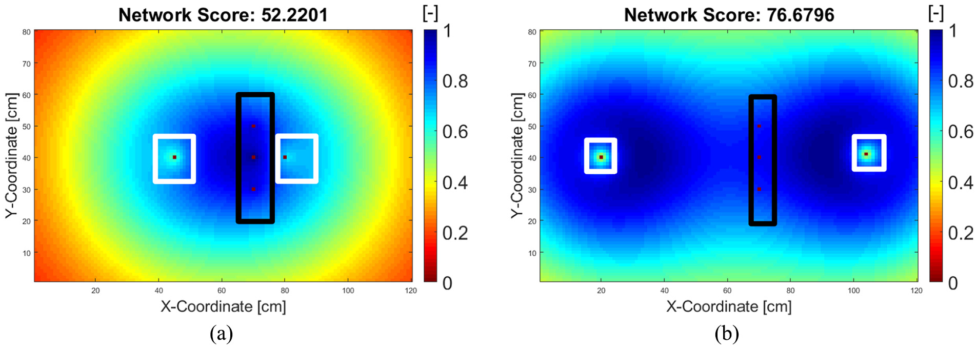
Network score for (a) hotspot SHM network and (b) stochastic SHM network.

However, as a side note, Figure 14(b) is an exception: we believe this sensor configuration would still have a good detectability of hotspot crack if we consider that the wave scatter from the rivet hole is coming in a perpendicular direction to the sensor (cf. Figure 8(c)). This would not be the case, for example, in Figure 12(d) to (f), where the sensors are not in the perpendicular position to the wave scatter coming from the rivet hole.

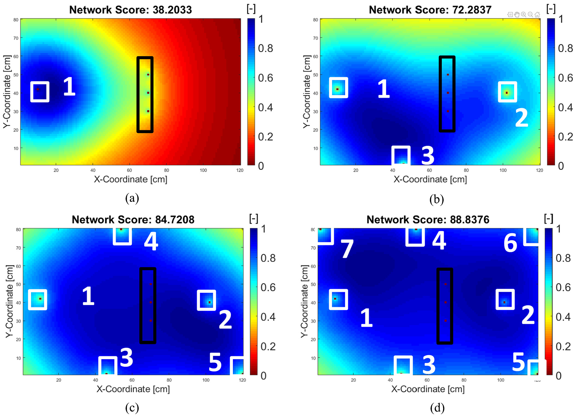
After first putting the two hotspot SHM sensors at 45|40 cm and 80|40 cm, the network score can be increased by adding several other sensors using the methods described in sections “Global random search” to “Preliminary conclusion.” This is demonstrated by adding 1, 2, 3, and 4 additional sensors, as depicted in Figure 15(a) to (d). Note that in these figures, the first- and second-best hotspot SHM sensors are denoted by numbers 1 and 2, respectively, and the locations do not change in every iteration.

Figure 15.

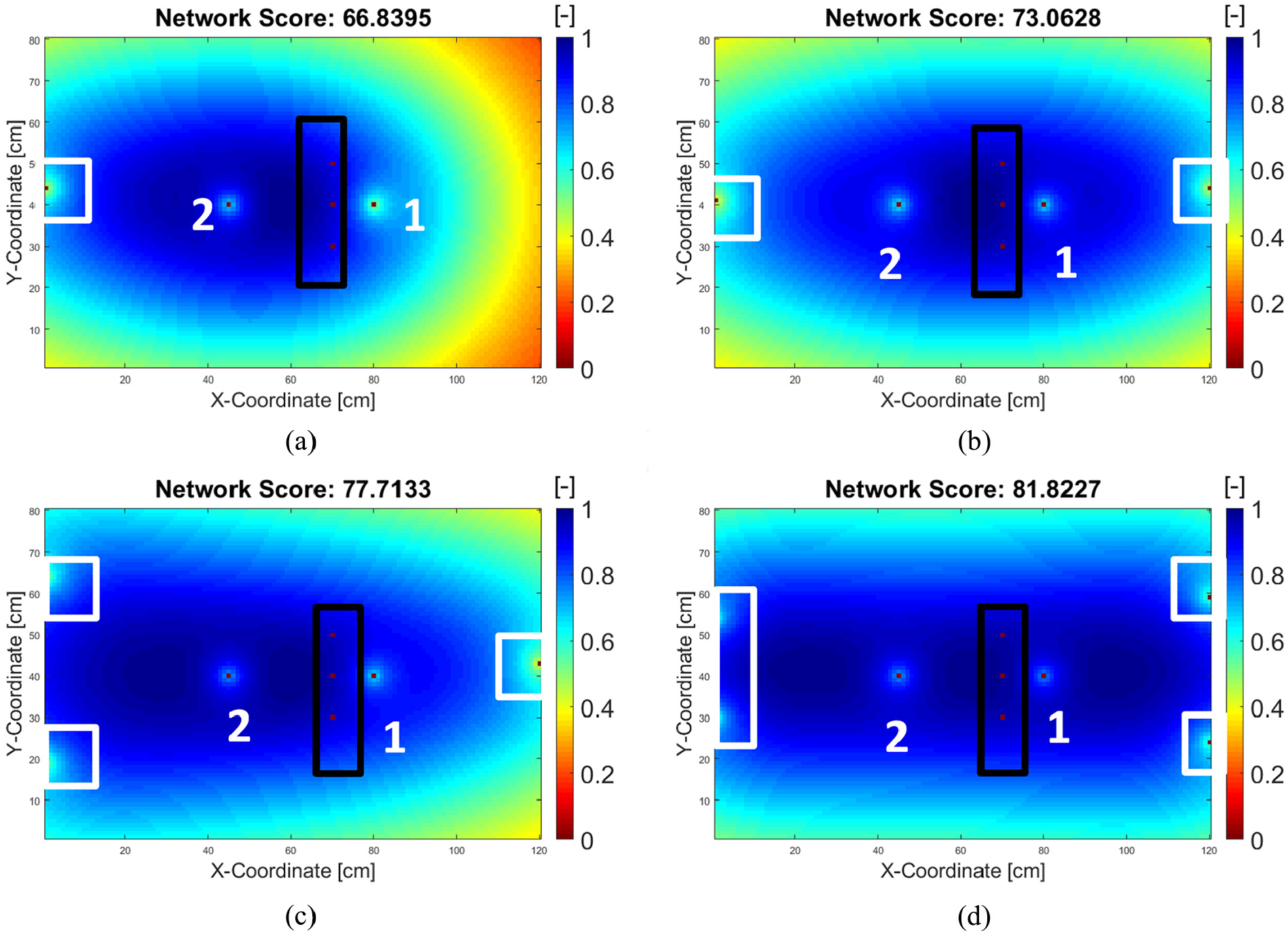
Network score for integrated SHM with 2 sensors for hotspot and (a) 1, (b) 2, (c) 3, and (d) 4 sensors for random damage detection, respectively. The first- and second-best hotspot SHM sensors are denoted by number 1 and 2.

The black and white rectangles signify the rivet hole and stochastic SHM sensor location, respectively. It can be concluded from Figure 15(a) to (d) that the network scores are lower than those from the solution generated by the pure GA; however, we think that this hybrid approach is the best way to compensate the conflicting objectives between hotspot and global SHM sensor placement.

Experimental validation

Experimental design

Hotspot SHM

As previously described in section “Methodology,” a hybrid approach that combines a hotspot and a global SHM sensor network design was made for an aluminum plate of size 100 × 50 cm with eight rivet holes using the simulation parameters given in Ewald et al. ²⁴ The hotspot location is assumed to be at 75|20 cm with a maximum damage tolerance size of a 16-cm fatigue crack (from tip to tip). Figure 16(a) and (b) depicts the wave propagation at t = 100 µs in the baseline and artificially cracked plate, respectively, where Figure 16(c) is the subtracted result of Figure 16(a) and (b).

Figure 16.

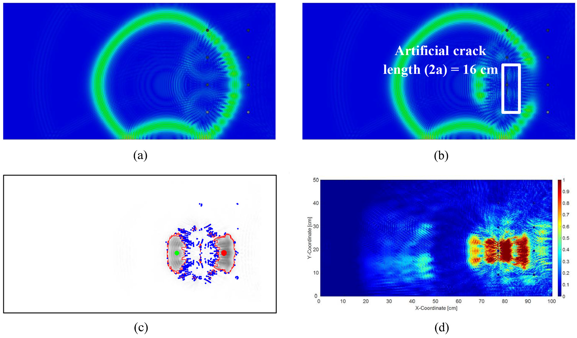
Simulated wave propagation in (a) baseline/pristine and (b) artificially cracked plate. (c) The subtracted result of image (a) and (b), where the centroids of largest and second-largest blob are marked by green and red dots, respectively. (d) Fused differential image from all time frames between 25 and 250 µs.

There are several blob centroids of interest, as depicted in Figure 16(c) and marked by the blue dots, where the largest and second-largest blobs are marked by green and red dots, respectively. The fused images from wave propagation times between 25 and 250 µs are depicted in Figure 16(d), and after averaging the blob centroids from all time frames, the best hotspot sensor coordinates found after using blob detection algorithm were 65|21 cm and 84|20 cm.

Integrated approach on global and hotspot SHM

After finding the hotspot sensors’ locations of 65|21 cm and 84|20 cm, the rest of the locations were determined by the GA. To minimize the number of PZT used in the experiments, we tested two sample networks: (1) 3 global + 2 hotspot sensors, and (2) 5 global + 2 sensors hotspots. For conciseness, the first network will be denoted as “3 + 2,” while the latter will be denoted as “5 + 2” from this point onwards. The sensor coordinates determined by the GA are depicted in Figure 17(a) and (b).

Figure 17.

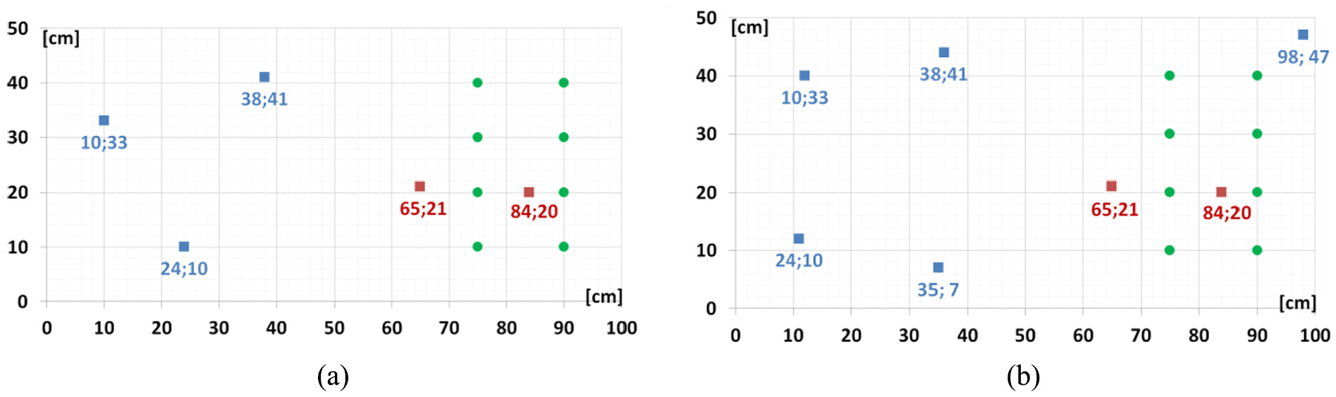
Sensor positions for (a) 3 + 2 network (scenario 1A) and (b) 5 + 2 network (scenario 1B). The red dots signify the hotspot sensors and the blue dots signify the rest of the global sensors that are determined by the genetic algorithm.

Multiple PZTs could additionally act as actuators to send excitation signals, and this would generate a larger dataset. Ideally, to reach the energy level that corresponds to the maximum network score, all actuators should be excited at the same time. For the 3 + 2 network, this would require five waveform generators. We do not have this amount of necessary hardware; therefore, for demonstration purposes, we only excited the hotspot sensor located at 65|21 cm; thus, only a fraction of the previously described signal power in equation (6) was used. The available hardware during the test were a Picoscope 6402A oscilloscope, an Agilent Waveform generator 33500B, standard BNC cables, a radial PZTs American Piezo APC-850 (Ø 9.52 mm, thickness = 1 mm, resonance frequency f_r = 207 kHz), and a desktop PC with Waveform Builder Pro and software from Picoscope installed. The experimental setup is depicted in Figure 18.

Figure 18.

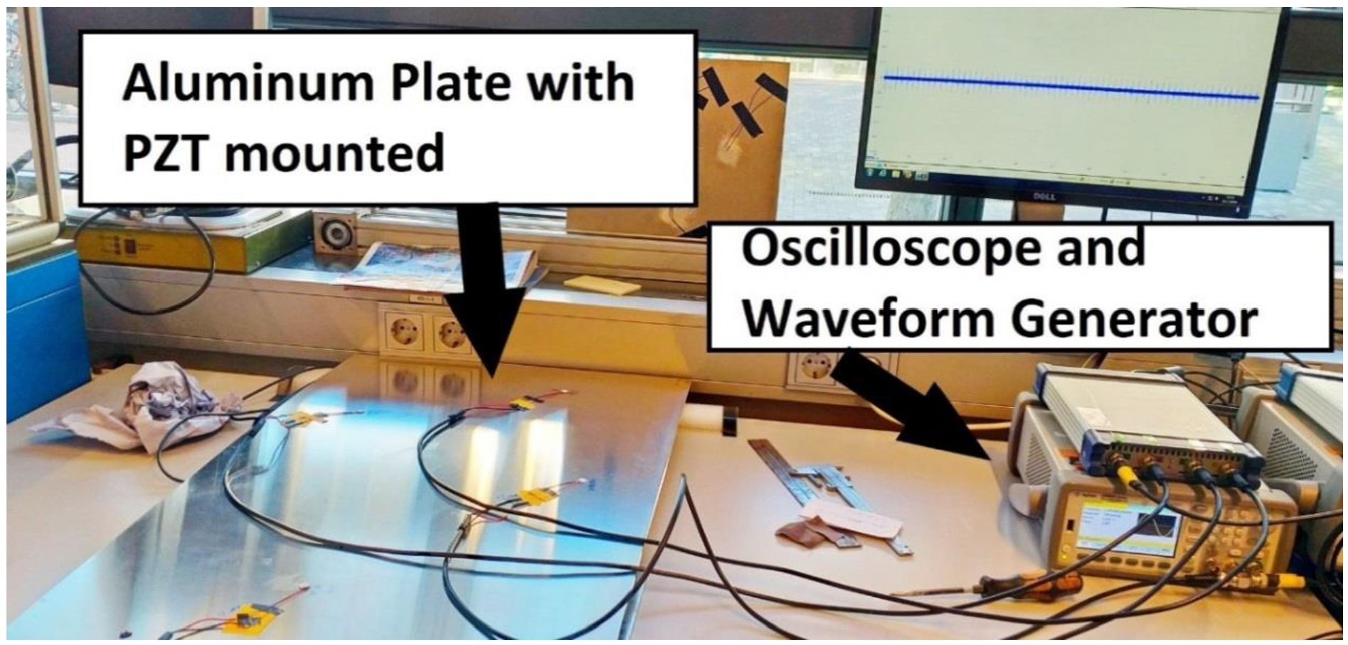
Experimental setup.

As we have radial mode PZTs with a thickness smaller than the diameter, normally it is the S₀-mode which is the predominant waveform that will be actuated and sensed by the PZT. ⁵¹ From eight specimens, two plates must be assigned as baseline; otherwise, the residual time-trace cannot be calculated. The baseline from the 3 + 2 and 5 + 2 network will be designated as scenarios 1A and 1B, respectively. As scenarios 2 and 3 have very large and visible damage (almost 30 cm), we can expect that the 3 + 2 network will be more than sufficient to identify this damage, and accordingly since scenarios 6 and 7 have a hardly noticeable barely visual impact damage (BVID), the denser 5 + 2 network is assigned to them. Finally, to compare the damage localization performance from both networks, the 3 + 2 and 5 + 2 network were assigned to scenarios 4 and 5, respectively.

Experimental details

In order to experimentally validate our sensor network configuration to detect both random and hotspot damage occurrences, we tested several damage scenarios as given in Table 2. An artificial fatigue crack was created by milling a slot adjacent to the rivet hole. The length of the artificial crack in a real application would be determined according to the damage tolerance criteria. For this study, we assumed it to be 8 cm from tip to tip, that is, including the rivet hole with a diameter of 1 cm.

Table 2.

Damage scenarios tested using aluminum 7075-T6 of size 100 × 50 × 0.2 cm.

Scenario	Heighth (m)	EnergyEImpact (J)	Velocityv (m/s)	Description of impact	Impact epicenter (cm)	Hotspot crack coordinates (cm)	Sensor network
1A	None These are baselines						3 + 2
1B							5 + 2
2	2.0	80.4	6.3	CVID, ca. ½ plate breaks	27; 24	None	3 + 2
3	2.0	80.4	6.3	CVID, ca. ½ plate breaks	27; 24	75; 20	3 + 2
4	1.7	68.4	5.8	VID, ca. ¼ plate breaks	20; 35	None	3 + 2
5	1.7	68.4	5.8	VID, ca. ¼ plate breaks	20; 35	None	5 + 2
6	1.6	64.3	5.6	BVID, only dent	27; 24	75; 20	5 + 2
7	1.6	64.3	5.6	BVID, only dent	27; 24	None	5 + 2

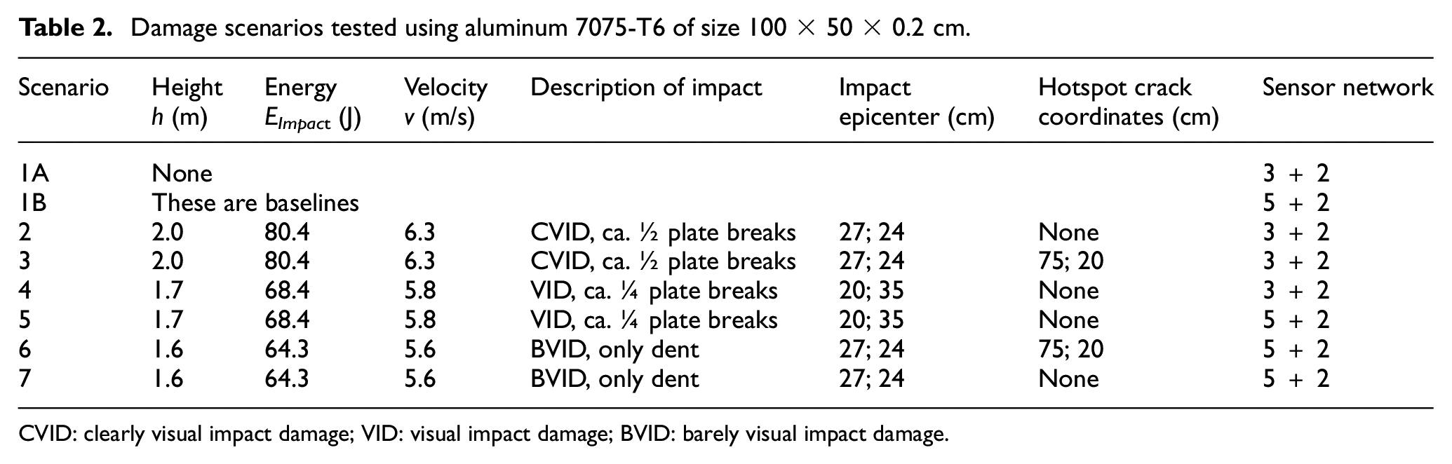
CVID: clearly visual impact damage; VID: visual impact damage; BVID: barely visual impact damage.

Due to the limitations of the dimensions of the fixation table of the impact tower (see Figure 19(a)), we reduced the dimensions of the plate to 100 cm × 50 cm as depicted in Figure 19(b) and repeated the procedure given in section “Integrated approach using blob detection and GA.” Depending on the impact type (hail impact, tool drop, ground collision), the impact energy could vary. For instance, a tool drop has a typical energy lower than 28 J, ⁵⁰ while hail impact energy during taxiing can reach up to 157 J ⁴⁹ and this can reach 3900 J ⁴⁹ during cruise. The TU Delft impact tower was operated at up to its height limit h = 2.0 m, which corresponds to an impact energy E_Impact of 80.4 J, as given in Table 2. This impact energy was sufficient to cause a large visible damage on the test coupon (see Figure 20(a)).

Figure 19.

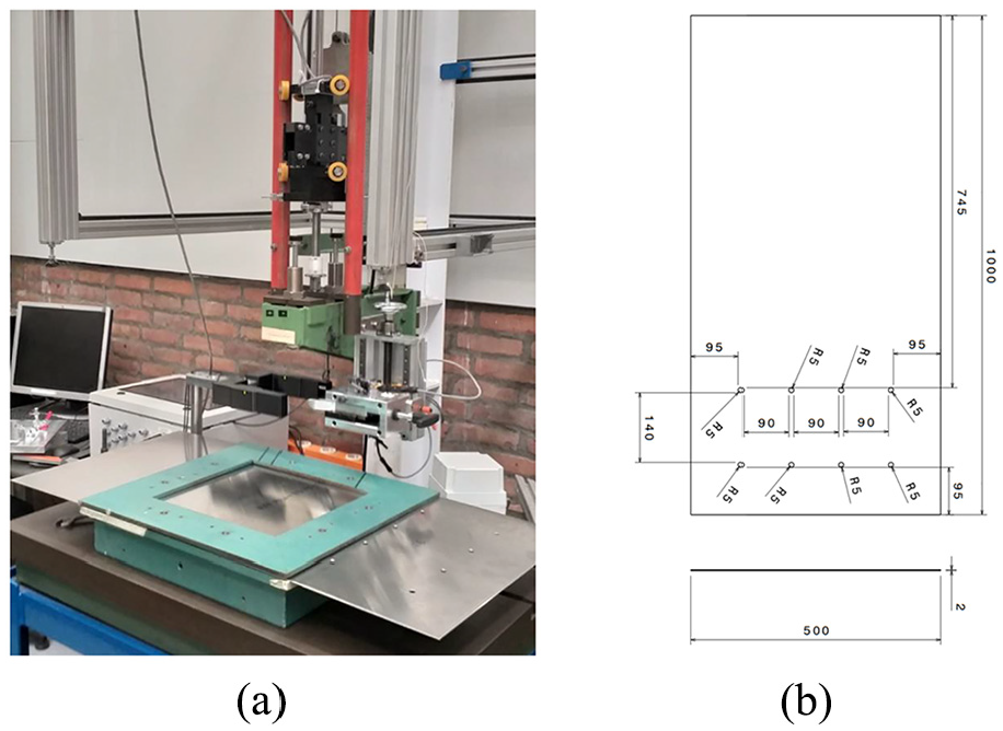
(a) Impact test setup and (b) dimension of the specimen in mm (including the rivet holes).

Figure 20.

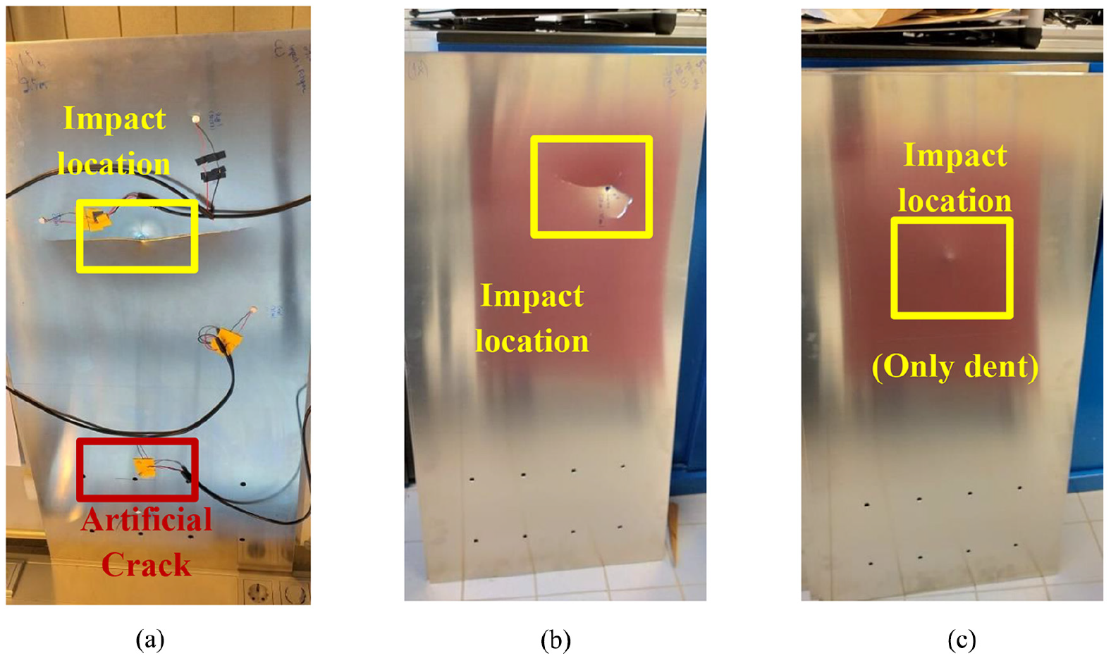
Example of damaged aluminum plates from scenario (a) 3, (b) 5, and (c) 7 of Table 1, respectively.

The maximum mass m that can be attached to the impactor is 2.4 kg (made of Tungsten), making the total impact mass 4.1 kg (including the mass fixation). During the testing period, a spherical impactor shape and fixator holder with sharp corner were available and thus were chosen. It is true that this mass is heavier than typical hail, but if we assume the potential energy E_Potential is fully converted to kinetic energy E_Kinetic this corresponds to impact velocities between 5.60 and 6.26 m/s—which is typically slower than hail impact even during taxiing. As an illustration, the damaged aluminum plates from scenarios 3, 5, and 7 are depicted in Figure 20(a) to (c).

Experimental result and discussion

To validate the consistency of each specimen setup, the cumulative CCs between the baseline and each damage scenario were calculated. The PZT pulsing actuation used the trivial 5-cycles Hann sinusoid (at f = 200 kHz), and the signal amplitude was recorded by the oscilloscope. As the hotspot sensor at 65|21 cm is used as an actuator, the only sensor which is available at the same location on every specimen is the one located at 84|20 cm. The normalized baseline signals, their envelope, and the corresponding cumulative CC are depicted in Figure 21. The CC can be calculated for any time length, for instance, the CC of the baseline signals and between the baseline envelopes until 300 µs are 0.9254 and 0.9366, respectively. This is to be expected, since even in an ideal experimental case, two similar and pristine plates can still have a difference in measurement due to material properties or in the presence of minor defects inside the materials.

Figure 21.

Baseline for scenario 1A and 1B at sensor located at 84|20 cm. The full results can be found in our Github.

Moreover, background noise and vibration from nearby equipment in the laboratory can cause a low-frequency signal oscillation. For this reason, we heuristically band pass the signal between half and double of the resonance PZT frequency (100–400 kHz) to isolate the low and high-frequency noise. Theoretically, an optimization on the band pass is needed; however, this was not the main purpose of our study. Since the plate dimensions are 100 × 50 cm and assuming that the S₀-mode is traveling at 5300 m/s, at 300 µs the wavefront would have covered a traveling distance of 2.12 m.

Fatigue crack detection

There is neither a need for damage localization nor damage classification for hotspot SHM placement as both the location and critical damage size will have been predicted according to damage tolerance design. Logically, only the SHM detection function applies here. As can be seen from Figure 22(a), there is an 80% decrease in the amplitude of both signals and the envelope between 36 and 53 µs, which corresponds to a traveling distance of 19 cm for the S₀-mode, which is exactly the distance between the actuator and the sensor. Accordingly, the CC of the signals and the envelope drops below 0.3 at 36 µs. Assuming that the measurement instrument is working properly (e.g. no defective cables or equipment), such a huge decrease in amplitude (80%) clearly signifies the lack of wave scatter in the propagation path between sensor and actuator. As such, it can be assumed that the crack emerging from the rivet hole has already blocked a significant portion of the wave propagation path. Figure 22(b) can be explained in the same way.

Figure 22.

(a) Scenario 1A versus 3 and (b) scenario 1B versus 6. The full results can be found in our Github.

Impact localization

While the detection of hotspot damage typically only requires an observation of amplitude change, impact localization also requires a signal observation regarding phase shift to extract information to calculate the travel distance of a particular Lamb wave mode. As an example, a comparison of the signal waveforms, envelopes, and their corresponding CC between the baseline (scenario 1A) and scenario 2 from network 3 + 2 at two different sensing locations are given in Figure 23(a) and (b).

Figure 23.

Comparison between signals waveforms, envelopes, and CC of the scenario 1A (baseline) and 2 (damaged) at the sensor located at (a) 84|20 cm and (b) 38|41 cm.

Since the CC_Envelopes only considers half of the signals and does not consider the incremental variation of the amplitude within the envelope, it is less sensitive toward the time shifts in the original signal waveforms, as can be seen in Figure 23(a) between 60 and 90 µs, marked in red dotted rectangle. On the other hand, CC_Envelopes is quite sensitive toward amplitude change, especially when the amplitude suddenly drops, such as between 180 and 200 µs, marked in Figure 23(b) in purple dotted rectangle. During this period, CC_Signal also drops, although this occurs in less dramatic way, that is, 0.9678–0.8713 for CC_Envelopes in comparison with 0.8337–0.7942 for CC_Signal. Figure 23(b) can be explained in the same manner.

As stated in the section “Experimental result and discussion,” the CC of the baseline signals and between the baseline envelopes until 300 µs are 0.9254 and 0.9366, respectively. For this reason, we can only consider that a damage would occur if the CC drops below these numbers. However, the CC would not only drop just because of the damage, we must consider all error propagation factors, such as an inhomogeneous amount of applied superglue between the PZT and plate surface, geometrical tolerances such as length, width, thickness of the plate and the rivet holes, the exact coordinate of the sensor placement, potential micro-defects within the plate, and so on. For this reason, it would be wise to consider a threshold CC that is slightly below these numbers, but still above 0.5 (CC = 0.5 means 50% correlation), otherwise all information that is contained below the threshold will be suppressed, too.

Along with the objective stated in section “Introduction” and Thiene et al., ¹⁸ the purpose of this article is definitely not to propose a novel signal processing method or new feature to calculate DI, but rather to propose a sensor network placement method that is DI-free and can be coupled with any signal processing. As an example, we consider a threshold of CC_Envelopes = 0.9 (which is <0.9254) and a CC_Signal = 0.8 (which is <0.9366). Thus, if both CC values drop below these thresholds, it is considered as significant. The original waveform and the signal envelope from the baseline (1B) and the damaged plate (scenario 5) and their CC captured by PZTs located at 12|40 cm and 11|12 cm is depicted in Figure 24(a) and (b).

Figure 24.

Comparison between signals waveforms, envelopes, and CC of the scenario 1B (baseline) and 5 (damaged) at the sensor located at (a) 12|40 cm and (b) 11|12 cm.

After determining the threshold, the first thing to consider is the time-of-arrival (TOA). Since both CC values are always changing every time increment, it is wise to take the TOA where the CC either (1) reaches its local optima or (2) stabilizes as a local plateau. For brevity, in both these cases CC is denoted as CC*. An example for Case (1) is given in Figure 24(a), where the TOA of the CC*_Signal and CC*_Envelope are at 124.0 and 128.6 µs, respectively. An example for Case (2) is given in Figure 24(b), where the TOA of the CC*_Signal and CC*_Envelope is at 120.9 and 150.8 µs, respectively. The TOA of course might change if the threshold is lowered or raised.

For simplification, we consider only the TOA of the first local optima and the first local plateau. In future work, the desired technique can be combined with more advanced signal processing however in line with our objective: we would like to know how well our hybrid sensor placement method works if it is coupled with conventional signal processing. The localization of the impact damage can be triangulated by calculating the elliptical distance between actuator and two different sensor positions, according to equations (17a) and (17b)

$$\begin{array}{c}\multicolumn{1}{c}{d_{S_0(\mathrm{Path}1)}=||P_{\mathrm{Actuator}}-P_{\mathrm{Damage}}||}\\ +||P_{\mathrm{Damage}}-P_{\mathrm{Sensor}1}||=v_{S_0}·\mathrm{TO}{A}_{\mathrm{Sensor}1}\hfill \end{array}$$

(17a)

$$\begin{array}{c}\multicolumn{1}{c}{d_{S_0(\mathrm{Path}2)}=||P_{\mathrm{Actuator}}-P_{\mathrm{Damage}}||}\\ +||P_{\mathrm{Damage}}-P_{\mathrm{Sensor}2}=v_{S_0}·\mathrm{TO}{A}_{\mathrm{Sensor}2}\hfill \end{array}$$

(17b)

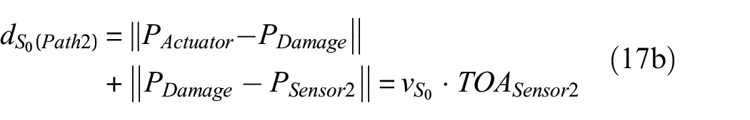
In equations (17a) and (17b), $d_{S_0(\mathrm{Path}1)}$ and $d_{S_0(\mathrm{Path}2)}$ are the sums of the Euclidian distance from the actuator to the damage and the damage to the sensor indexed with location 1 and 2 measured from each position P of either the actuator or damage, respectively. P_Actuator, P_Sensor, and P_Damage are the x- and y-coordinates of the actuator, corresponding sensor, and damage, respectively. $v_{S_0}$ and TOA_Sensor are the velocity of the S₀-wavemode and the time of arrival at the corresponding sensor location, respectively. P_Damage can be obtained by solving equations (17a) and (17b) simultaneously. By repeating this step for all actuator–sensor pairs, a distribution of predicted P_Damage can be obtained. For every solved quadratic equation, there are a maximum of two solutions. An example of these calculations using TOA from CC*_Envelope for a single actuator–sensor pair is given in Table 3. Note that the full table is too long to be presented here.

Table 3.

Predicted damage location based on TOA-triangulation from various damage scenario.

Scenario	x-y-Coordinate (in cm) of			TOA of CC*Envelope (in µs) from		Predicted damage x-y-coordinates (in cm)
	Actuator	Sensor 1	Sensor 2	Sensor 1	Sensor 2
2	65|21	84|20	10|33	197.9	113.7	22|26 OR 21|39
3	65|21	84|20	24|10	40.5	131.4	79|78 OR 16|25
4	65|21	24|10	10|33	200.5	110.7	Complex Root
5	65|21	84|20	12|40	202.3	128.6	21|31 OR 18|52
6	65|21	35|7	36|41	208.9	150.8	22|56 OR 59|67
7	65|21	84|20	12|40	204.3	131.4	21|31 OR 17|53

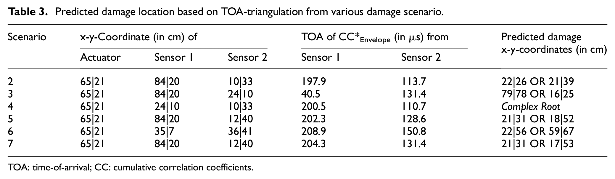
TOA: time-of-arrival; CC: cumulative correlation coefficients.

Not every single solution is useful, for instance, in scenario 1A–3, the first predicted coordinate at 79|78 cm, which lies outside of the plate; thus, the other solution which is at 16|25 cm is taken as the accepted predicted location. In scenario 1A–4, both solutions are complex roots so they cannot be considered anymore. In this case, only the roots that fulfill the constraint (i.e. positive real numbers within the dimensions of the plate) are taken as an accepted solution.

The reason that sometimes there are no accepted solutions is because in equations (17a) and (17b), all TOA(CC*) are multiplied by S₀-wavemode velocity since we assume that the dominant Lamb mode for excited radial PZT is the S₀-mode. This is an oversimplification because generally, both fundamental Lamb modes are always present, that is, after the wavefront encounters inhomogeneities such as rivet holes and plate boundaries, wave mode conversion occurs. To avoid this, a Lamb wave mode separation technique such as Xu K ⁵⁶ can be used to sort in which group the TOA belongs to. For now, it is enough to consider all accepted predicted damage locations and to calculate the distribution of these predictions. The distribution of the predicted damage locations is summarized in Figure 25(a) to (d), which shows predicted damage locations from scenarios 2, 4, 5 and 7, respectively. As can be seen from Figure 25(a), even a simple algorithm can easily localize a large damage size (about ½ of plate impacted).

Figure 25.

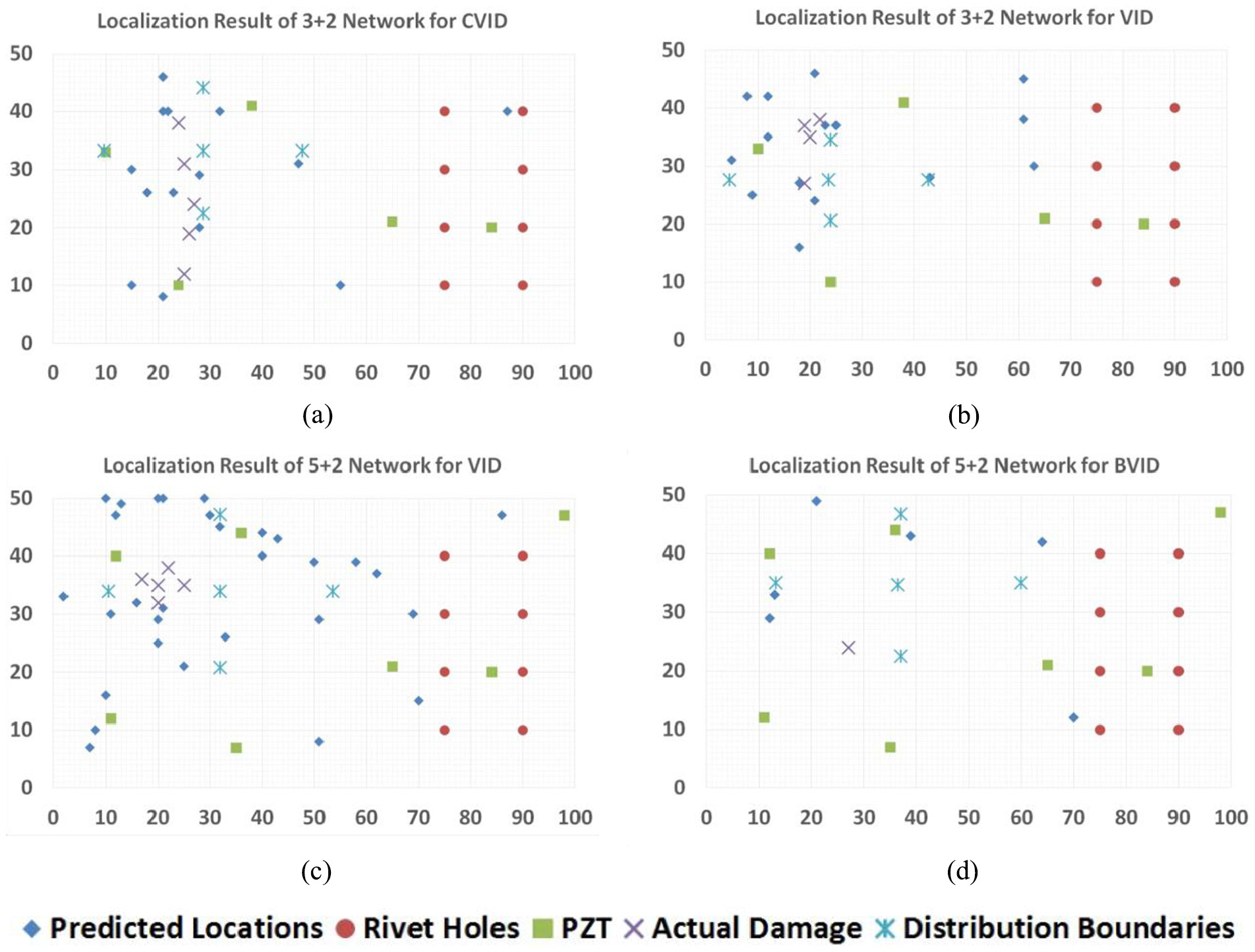
Damage localization result from scenario (a) 2, (b) 4, (c) 5, and (d) 7.

As can be seen from Figures 25(a) and 26(a), the simple algorithm can easily localize a large damage size (about ½ size of the plate height, that is, 30 cm), although there is an area that was not covered by the distribution as the damage itself is quite large. Furthermore, for the localization of smaller impact damage (about ¼ plate, that is, impacted in scenario 4 and 5) which are depicted in Figure 25(b) and (c) and Figure 26(b) and (c), respectively, the determination of damage location based on TOA calculation outputs provides a relatively reliable localization. This is in contrast with BVID, which barely causes a smaller dent on the surface where in this case, even the denser network is not able to predict the damage location in a sufficient manner as depicted in Figures 25(d) and 26(d). Taking a closer look into the quantification of the localization performance, we calculated several criteria as given in Table 4 as follows:

1. Averaged Euclidian distance δ : the distance between each predicted damage location P_x, _y (which is just the distribution mean) and the epicenter of the actual damage epicenter A_x, _y without considering the multi-site damage;

2. Mahalanobis distance M : the distance between actual damage epicenter without considering the multi-site damage and the probability distribution of all predicted damage locations;

3. Standard deviation σ_x and σ_y for both x- and y-axis;

4. Percentage R which is ratio between elliptical area covered by vertex σ_x and σ_y divided by plate size, which is 100 × 50 cm = 5000 cm², for scenario 2, 4, 5, and 7: these elliptical areas can be seen in Figure 26 already.

Figure 26.

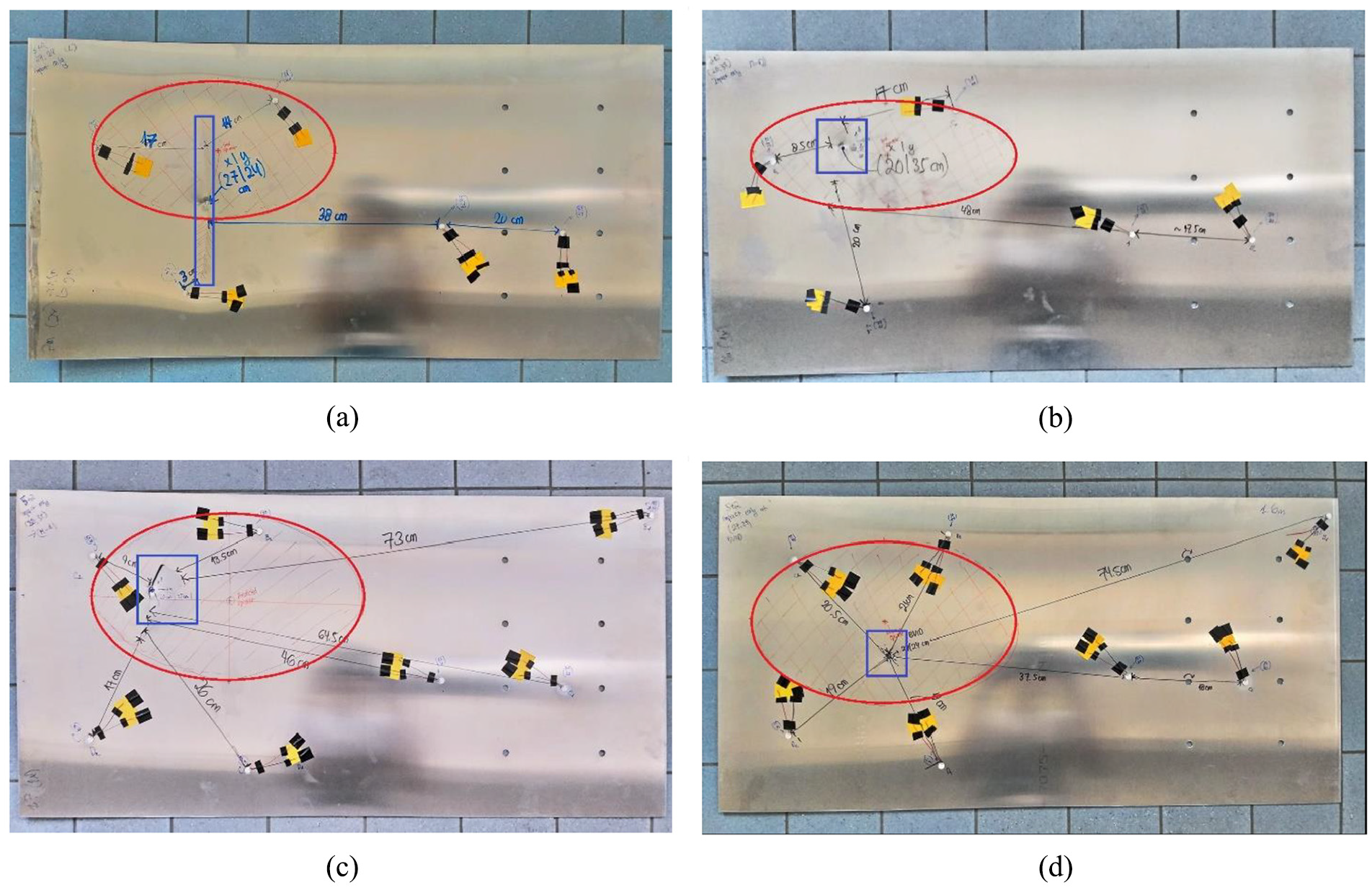
Real plate from scenario (a) 2, (b) 4, (c) 5, and (d) 7. The blue rectangles indicate the impact damages where the red ellipse are the distributions of predicted damage locations.

Table 4.

Euclidian and Mahalanobis distance between the predicted and actual impact epicenter.

Scenario	Ax, y (cm|cm)	Px, y (cm|cm)	δ (cm)	M (unitless)	σx|σy (cm|cm)	R
2	27|24	29|33	9.5	4.438*10−3	19|11	13.0%
3	27|24	24|28	5.0	4.665*10−3	19|7	8.3%
4	20|35	27|34	6.8	2.990*10−3	20|8	10.2%
5	20|35	33|33	12.8	3.824*10−3	21|12	16.2%
6	27|24	26|30	5.8	2.033*10−3	21|13	17.2%
7	27|24	37|35	14.3	1.531*10−3	23|12	17.8%

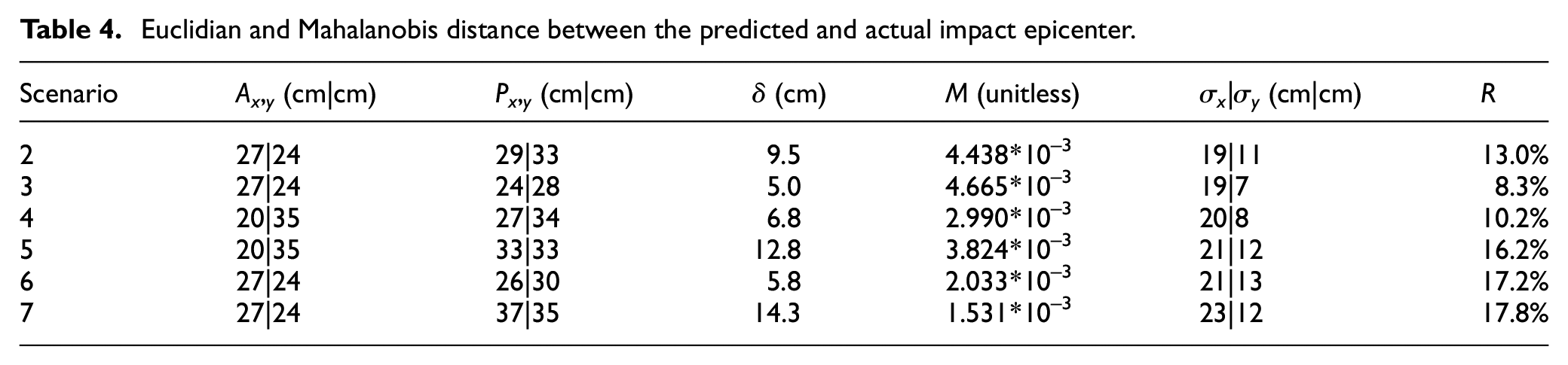
As it can be seen from Table 4, the Euclidian distances between the predicted and actual epicenter vary between 5.0 and 14.3 cm. Note that in scenario 2–5, the damage is quite large, that is, not only dents and therefore it occupies multiple locations and the actual damage locations are covered by R. In scenarios 6 and 7, R is large, but the damage size is small (dents Ø = 1 cm), which poses a limitation of the damage detection algorithm, because the Lamb wave mode at this particular PZT frequency (200 kHz, wavelength λ = 2.65 cm) is not a good match with the damage size. The difference between scenarios 6 and 7 is only the artificial fatigue crack located at 75|20 cm for scenario 6, as described in section “Fatigue crack detection.” For scenario 7, the average error on Euclidian distance is 14.3 cm and the ratio R is 17.8%.

Practically, if scaling our approach for a larger-sized structure (e.g. 5 × 5 m), then at least 4 m² (about ⅙ or 16.7% of the surface) must still be scanned manually. As stated previously, our sensor network pattern is designed to work independently of any signal processing; thus, to increase accuracy in the future, the signals could be first separated using method described in Xu ⁵⁶ and then processed further using the delay and sum method for sparse reconstruction described in Nokhbatolfoghaihai. ⁵⁶

Thus, when scaling up our results to a business case, the approximated reduced man-hours using the integrative approach is about 83%, even if our sensor network is less dense than those proposed by Soman and colleagues^19,55 and Ismail et al. ²⁰ In Soman and Malinowski, ⁵⁵ they suggested that for nine sensors, an area 90.2% within an aluminum plate with a size of 1 m × 1 m if the coverage is defined as the percentage of an area that lies in the sensing range of a single sensor–actuator pair. A further adaptation for sensor density must be considered if a temperature change is involved as reported by Croxford et al. ⁵⁶ They reported that for a small temperature change (less than 1°C), 5 sensors/m² in an aluminum plate is enough for baseline subtraction in pulse-echo technique with 1-MHz central frequency. The density becomes absurdly high (97 sensors/m²) if a large temperature change (more than 10°C) is introduced. Fortunately, Lamb wave SHM with a central frequency higher than 500 kHz is very rare as such high-frequencies will typically induce the unfavorable higher-order Lamb modes, especially in a plate thicker than 4 mm.

Clarke ⁵³ and Croxford ⁵⁵ considered that SHM systems to be successful if those combine (1) good sensitivity to defects, that is, good damage detection capability, and (2) preferably with localization and identification, with (3) a low sensor density. While such a denser network as has been proposed by Soman et al.^19,55 and Ismail et al., ²⁰ we think they may increase the sensitivity and thus can reach at least 95% man-hours reduction—however, on the other side, the investment cost must also be taken into consideration. If the investment cost overweighs its benefit, we start to doubt the practicality and the usefulness of the SHM system when the SHM system is intended primarily to reduce the maintenance cost.

Furthermore, we believe this figure tends to be overestimated because in airline operation, many unpredictable things occurred (sensor dies, oscilloscope is broken, cable is torn, etc.). In a worst case where we can only reach 50% of the promised reduced man-hours, the integrative approach would still count 41.6% instead of 83% man-hours reduction. Airlines typically spend around 30% of their budget for the maintenance, so if the man-hours are reduced by 41.6%, this would still save them at least 12.5% of the operating expenses. This is a very broad figure, but we can expect the calculation above to be quite realistic.

It is often forgotten that the purpose of SHM is not to replace NDT completely, but to determine whether a further NDT inspection of a certain aircraft part is needed during unscheduled maintenance or not. Therefore, we believe that by reducing the inspection man-hours by at least 41.6%, we consider that our hybrid sensor placement method with a minimum number of sensors for hotspot and global damage detection contributes to design strategies for Lamb wave SHM.

Conclusion

In this work, we demonstrated that a sensor network topology for hotspot SHM for detection of predictable crack location can be merged with the probabilistic approach without sacrificing too much of the global sensitivity. To do so, first, the hotspot sensor locations are determined according to the largest centroid based on blob detection algorithm. To determine the sensor positions for detecting random damage, three search algorithms were compared: global random search, greedy, and GA. Global random search has the lowest performance, and the GA has the best performance. Accordingly, as per the No Free Lunch Theorem, the GA took the most computational resources—this can be either in time or space while the random search took the least computational resources. The performance and required computational resources of the greedy algorithm lies in between global random search and the GA.

Since the specimen size used in our work was not too large and the computational time for every iteration search was below 1 h, we decided to use the GA to determine the global sensor positioning. It is also worth to mention that, in line with Mallardo et al., ¹⁷ our results suggest that global sensor positioning tends to work well in an open area but not very suitable for complex geometry such as placement close to stringers and fasteners. The reason the GA is placing sensors in impractical locations is due to unprecise engineering constraints formulation; thus, the GA search space becomes very large. Our recommendation for future work is thus a more precise engineering constraints definition.

Nevertheless, with this hybrid approach, we demonstrated that sensor networks can detect fatigue cracks and locate randomly occurring damage, if these do not occur at the same time. We believe this likelihood is small, but nevertheless, it might be interesting in future study to understand the probability of fatigue crack and impact occurring at the same time.

Given the results in section “Experimental result and discussion,” we consider that our hybrid approach based on blob detection algorithm and search metaheuristics can partially address sensor positioning problem in active ultrasonic SHM in scalable manner—especially when the detection requirement is not too high (such for BVID). However, for placing a much larger numbers of sensors in a larger and complex structure, we suggest using the greedy algorithm instead of the GA to compensate for the network performance and the computational effort required.