Sage Journals: Discover world-class research

Abstract

The method herein proposed provides a novel perspective about data processing within structural health monitoring, which is essential for automated real-time monitoring and assessment of civil engineering structures. The low- and high-frequency contents of the forced vibration response of a structure are used to train and test artificial neural networks for the purpose of damage detection. In the context of several damage scenarios, the different versions of the networks are compared with each other with the aim of verifying which are the most efficient regarding novelty detection (one-class classification). The data related with the high-frequency response showed to contain more useful information for the proposed damage detection algorithm, when compared with the low-frequency response data (typically modal). In view of that, high frequencies should be given more attention in future research about their application in connection with structural health monitoring systems.

Keywords

Structural health monitoring artificial neural networks damage detection data-based method high-frequency response analysis

Introduction

Disasters involving bridges still take place these days, even though circumstances indicate that it should be progressing in the opposite direction with evolved technology and sensing devices, as well as with the stricter safety measures and maintenance procedures practiced nowadays. Very recently the abrupt collapse of the Morandi Bridge¹ in Genoa, Italy, which caused the death of 43 people, has revived the concern regarding the conservation of existing bridges in operation. A preliminary investigation links the bridge collapse to a combination of poor design, questionable building practices, and inadequately planned or implemented maintenance. Hopefully, this unfortunate incident (Figure 1) will trigger or reestablish the investment in such infrastructures, mainly in maintenance work, which has dropped significantly in some European countries in the last years (Figure 2).

Figure 1.

Morandi Highway Bridge collapse in Genoa, Italy.

Figure 2.

Genoa bridge collapse. The graph shows that Italy has slashed its investments in infrastructures.

Within structural engineering, structural health monitoring (SHM) consists of a number of practices and strategies that permit the acquisition of information about the current state of a structure and to make future predictions when implemented. Monitoring should be incorporated into the inspection system, with the advantage of continuously producing information that can be later used and compared with new measurements. The need for monitoring of a structure can be motivated by varied reasons—damage, bearing capacity, remaining lifetime, passenger comfort, and so on—the first of which sets the focus of this article. A big part of what damage detection is about deals with identifying what characteristics of the structure better express the presence of damage, if it is present—the so-called damage features. These features can be extracted from measurement data, directly or indirectly, which nowadays can be collected in massive amounts. It is thus important to reach an understanding on what parts of the data are actually crucial to retain for the damage detection process and what parts can be dismissed. These parts can be obtained from the whole measured signal through the application of signal processing techniques, for example frequency filters.

Damage identification techniques in civil engineering structures, including bridges, have consistently focused on the monitoring of modal-based damage sensitive features, as these are directly related to intrinsic parameters of the structure such as its stiffness. Validation is carried out mainly through numerical validations and these normally limit themselves to modal data. There is a good understanding of the modal data and thus, traditionally, focus is put on the lower part content of the frequency spectrum. However, damage is typically a local phenomenon, and it is known that local response can be captured by higher frequency modes² while the global response is captured by the lower frequency modes. This is evident in Khoa et al.³ with the case study of the Sydney Harbour Bridge. When comparing the frequency response function (FRF) of the structure between the measured responses obtained from the healthy and damage cases, it is observed that the damage effects are more visible at high frequency.

Several works exist about the effectiveness of methods that use high-frequency excitation for structural deterioration and damage detection. Within the high-frequency range, the wavelength of the excitation is small and sensitive enough to notice minor changes in the integrity of the host structure. In Heckman,⁴ for example, high-frequency seismograms are used for damage detection when the presence of damage produces high-frequency signals. These occur, for example, due to the acoustic emission that occurs during crack propagation or after damage as already occurred, with the opening and closing of the crack. In Yan and Chen,⁵ high-frequency piezoelectric signatures via the reverberation matrix method are used to perform quantitative damage detection. Numerical simulations show that the impedance spectrum is capable of identifying some new resonant peaks due to local damages growth in the high-frequency range.

The SHM problematic, more specifically in a context of pattern recognition, can be broken down into four parts:⁶ Operational Evaluation; Data Acquisition, Normalization, and Cleansing; Feature Extraction and Data Compression; and Statistical Model Development. These previously mentioned works mainly target an investigation within part 2—Data Acquisition—which includes the selection of suitable excitation and measurement methods. However, to the present knowledge of the authors of this article, literature directed at looking into the high-frequency response of the excited structure for damage identification is scarce or unavailable. Such investigation would pertain to part 3—Feature Extraction and Data Compression—that deals with the selection of the best features for damage detection, among other aspects that follow data collection.

A method for SHM and damage detection supported by machine learning is proposed in this article. The novelty and focus is placed on the study of the frequency content of the measured forced vibration response signal (limited to accelerations in this article) and how that affects the quality of the damage detection process. Numerical and experimental case studies are investigated in order to validate the proposed method. Recognition that the success in damage detection using the proposed method is greater when only data associated with high-frequency response is accounted for in the learning process (opposite to only low-frequency response) can be important. Such finding could change the way how damage detection methods in SHM, typically designed in terms of modal parameters, are implemented and accentuate the potential of databased methods supported by machine learning.

Damage detection using SHM

Damage present in a structure is expected to yield changes on its dynamic properties that can be perceived on the structure’s response: onset of cracks, loosening of bolted joints, corrosion, and fatigue. For instance, natural frequencies are relatively easy to measure, and significant changes can be used to identify damage. Depending on the complexity of the used techniques and detail in the collected information, a further robust SHM system may permit to reach the higher stages of damage identification,⁷ such that it is possible to localize and quantify the extension of damage.

Methods for damage detection

Well-established theoretical-based methods that apply such techniques are known as vibration-based damage detection (VBDD) methods, and their applicability for damage detection in civil engineering structures has been substantial as shown by an extensive repertoire of papers.^7–9 The underlying idea behind VBDD methods is that damage-induced changes in the physical properties of the structure (mass, damping, and stiffness) will cause detectable changes in the modal properties (natural frequencies, modal damping, and mode shapes). As such, damage can be identified by tracking changes in the normal vibration of the structure. These methods have therefore the advantage of delivering results that are quite intuitively interpreted. Other advantages are that the location of damage does not need to be known a priori, contrary to what happens to local damage detection methods (e.g. ultrasonic). Yet, as mentioned earlier, damage is a local phenomenon. This downside can affect the application of VBDD methods as, from a testing standpoint, higher frequency responses of the structure at ambient conditions are more difficult to excite since more energy is required to produce measurable response at those range of frequencies. Moreover, the easily extracted lower sensitive modes are quite sensitive to changing environmental and operational conditions.¹⁰

If a model is to be used for damage detection, for example, based on the finite element method (FEM), the accurate modeling and the development of a robust inverse algorithm are fundamental. However, FEM has as a major disadvantage that a large number of finite elements and nodes ought to be involved for accurately predicting high-frequency response of a structure. As the finite element model mesh becomes finer, the associated mass and stiffness matrices grow in size, creating large needs of storage and computing time. Moreover, the higher frequency content that can expose existing damage is sensitive to local conditions and geometry, which is often unknown or omitted during numerical modeling.

Alternatively, local techniques such as acoustic emissions¹¹ or guided ultrasonic waves¹² can perform damage detection with great precision but are quite expensive as these methods require high-tech hardware as well as well-trained operators, becoming just inconceivable for large structures.

Nowadays, artificial intelligence and machine learning are all the more applied to solve problems in several engineering branches, including civil engineering. Algorithms can be developed and used for feature extraction, data normalization, classification, regression, and statistical model development with artificial neural networks (ANNs) being one of the most commonly used algorithms. ANNs trained with dynamic data gathered from a healthy structure seem to successfully predict the healthy dynamic behavior of said structure. These predictions can be compared with the actual future measurements on the structure, and if significant differences are found above a specified threshold one can be confident that the structure is behaving differently than normal and that damage may be present. Used together with well-established statistical methods, these emerging machine learning techniques can certainly become helpful in the field of SHM.

Signal processing and filtering

Vibration is typically characterized by three parameters—displacement, velocity, and acceleration—and the sensitivity of the sensors that measure said parameters varies with the frequency of the vibration. According to Tsang,¹³ the general practice is to use displacement reading sensors with low-frequency signals, velocity reading sensors with signals in the middle ranges of frequency, and acceleration reading sensors with high-frequency signals.

Filtering can be used to improve the quality of SHM as most monitoring systems handle data that contain not only the original testimony of the structure’s behavior, which can lead to damage detection, but also the undesirable distorting issues such as those caused by noise from sensor sources and changing environmental and operational conditions. As such, Figure 3 describes the several possible uses of filters when defining the input for the algorithm, which will be investigated in this article.

Figure 3.

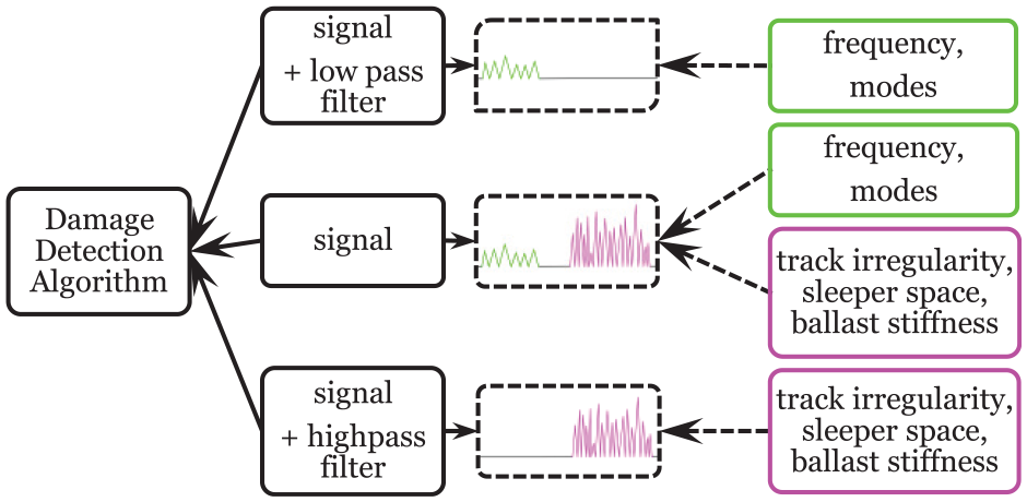
Three possible inputs for the algorithm.

Methodology

In this section, the methods comprising the proposed approach are presented and described.

ANNs

ANNs trained with measurement data acquired in a healthy structure can help to predict the expected normal behavior of the structure.¹⁴ The predictions respecting the baseline behavior can be compared with future measurements on the bridge. If significant differences are found above a specified threshold, a fault analysis alert will be triggered, based on which one can estimate the likelihood of the structure being damaged and act upon that information. 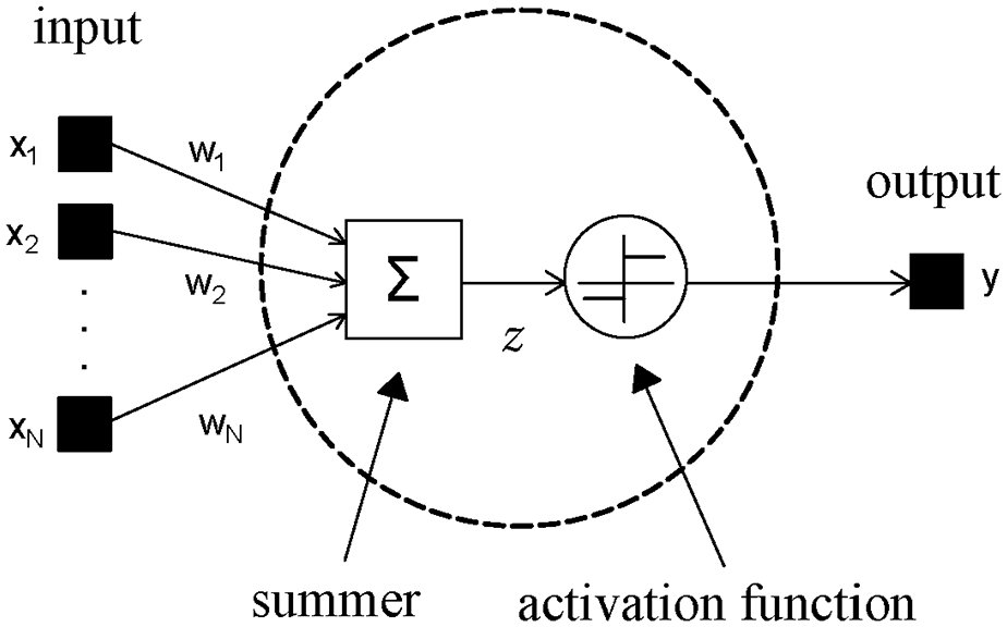The ANN structure is made of neurons (Figure 4) and layers (Figure 5), in a nutshell: inputs $x_{N}$ are multiplied by corresponding weights $w_{N}$ (a bias term can added) before being passed to the body of the neuron and summed together. The sum $z$ is then passed through a nonlinear activation function within the commonly used step function (Heaviside) linear, logistic (sigmoidal), and hyperbolic tangent functions. The neuron fires, that is, passes the signal to the next neuron, if the weighted sum $z$ exceeds some predefined threshold.

Figure 4.

Model of the artificial neuron.

Figure 5.

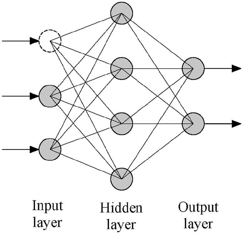
Layers of the artificial neural network.

The proposed method is validated with two case studies: one with a numerical model of a bridge and another with measurements collected from an existing bridge. In the former, train passages with similar characteristics are simulated over healthy and damaged scenarios to generate dynamic response data. ANNs are taught to learn the structural reference behavior based on the generated healthy data. The training data in the case study will be limited to the vertical accelerations of the bridge deck, but it could also be extended to strain, temperature, humidity, and so on. ANNs have normally one input layer, one hidden layer, and one output layer, and the number of input neurons is determined by the number of features in the training data: if, for example, 10 acceleration inputs are given then the network will have 10 input neurons. Empirical rules-of-thumb¹⁵ exist for determining how many hidden neurons there should be. Further description about the ANNs training process can be found in subsections “Model aspects and uncertainties,”“Data collection,” and “The ANN” under the “Case study I: numerical experiment” section in this article.

Performance of the method for damage detection

Once the ANN is trained, its predictions can be compared with future actual measurements on the targeted structure or with model generated data (both healthy and damaged), where significant differences given as the root mean squared error (RMSE) may indicate the presence of damage. The information coming from the several sensors can be combined (equation (1)), and the condition of the structure can be quantified by one number—a damage index (DI). One possible way to carry out this combination is through the Mahalanobis distance,¹⁶ which gives a measure of the distance between a point P and a distribution D. The distance is a measure of how many standard deviations P is from the mean of D. The equivalent reasoning in light of the case studies is that we compare each newly obtained DI (in healthy or damage conditions) to the cloud of DI points that we take as the reference (in healthy condition). Therefore, the DI is given according to the expression

DI (s) = \sqrt{{(RMSE (s) - μ (s))}^{T} . {σ_{xy}}^{- 1} . (RMSE (s) - μ (s))}

(1)

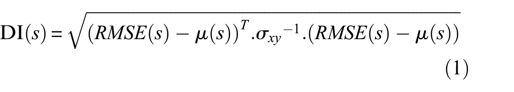
where, for each train speed $s$ (equivalent to one train passage), $RMSE$ is the prediction error, $μ$ is the mean prediction error of the reference distribution D, and $σ_{xy}$ is the covariance matrix of the reference distribution D.

In a second phase, low-pass (LP) and high-pass (HP) filters with appropriate cutoff frequencies are applied to the original measured healthy data and the ANNs are retrained for each case. The performances of the method based on each of the three ANNs (unfiltered, LP, and HP signal) are compared with each other.

Despite the many positive outcomes, it is not fully understood how the ANNs learn from the training data samples. ANNs are in fact seen as black-box models,¹⁷ contrasting with more interpretable models such as regression and decision trees. The black-box issue, in a sentence, consists of the following: the approximation given by the ANN will not give any insight on the form of f, the function being approximated. There is no simple link between the weights of the inputs and f. Even the analysis of which input characteristics are the most important is an open problem and thus, for a better grasp on this, an iterative trial–error process is in some way necessary. This means that while using the whole signal for the learning process it is basically impossible to tell which part of the signal the ANN puts more focus on, that is, which parts of the signal are the richest in information in what concerns the damage features. One way to perform such verification is by applying several signal processing techniques to the data prior to the learning process and then, evaluate which produce changes in the results, for the better.

The dependency of the DI on the chosen threshold, while having into consideration correct and incorrect diagnosis, can be represented graphically. The receiver operating characteristic (ROC) curve (Figure 6) is a graphic that illustrates the performance of a binary classifier (in this case the ANN) as a function of an adjustable threshold, showing exactly the information that is of prominence in problems of damage detection. To be more specific, the ROC curve shows the information about type I and type II errors for all the possible choices of the threshold. A type I error, also known as false positive (FP), occurs when a healthy structure is deemed as damaged. On the other hand, a type II error, also known as false negative (FN), occurs when existing damage in a structure goes undetected. In Figure 7, for illustration, a threshold is chosen such that the percentages of true and false classifications are TP = 83.3%, TN = 94.7%, FN = 16.7%, and FP = 5.3%. The threshold can be adjusted according to the maximum acceptable error of each type. If, for example, FNs are believed to be associated with worse consequences, under certain circumstances, then it may be sensible to raise the threshold in order to decrease this type of error. At the same time, this decision will adversely result in the increase of FPs. It is important to keep in mind that one ROC curve is suitable for a unique damage scenario, meaning that the ROC curves for two distinct damage scenarios will be different. In principle, a more severe damage will amplify the difference between the behaviors of a healthy and a damaged structure, thus making the existence of damage more detectable. In other words, one expects the false classifications (FPs and FNs) to decrease with increasing damage severity. Naturally, additional factors come into play as well and the location of damage in the structure is one of them.

Figure 6.

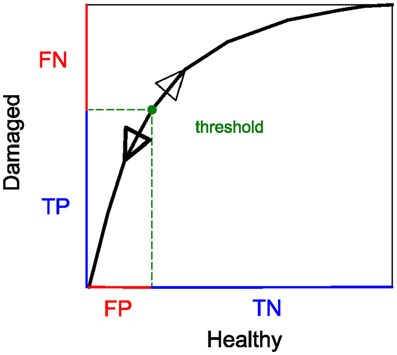
Generic receiver operating characteristic curve.

Figure 7.

Different detection thresholds () for the prediction errors obtained for a number of observed healthy () and damaged () samples yield different percentages of true (TN and TP) and false (FP and FN) classifications.

The frequency range of the signal

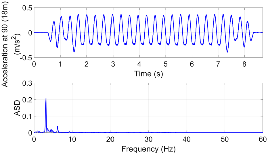
The raw unfiltered data cover a range of frequencies: the lower frequency response associated with the modal properties of the structure such as modal stiffness and damping (Figure 8); the higher frequency response associated with track irregularity and train–track–bridge interaction (TTBI) phenomena (Figure 9). It can be seen how important it might be to take into account these last aspects that arise in reality—if considered, the strength of the energy in the amplitude of the spectrum increases at higher frequencies where variations in the signal become stronger, as shown by Figure 9. The upper representation shows a time series signal (in this case, the vertical acceleration at a certain section of the bridge), and the bottom displays the amplitude spectral density (ASD).

Figure 8.

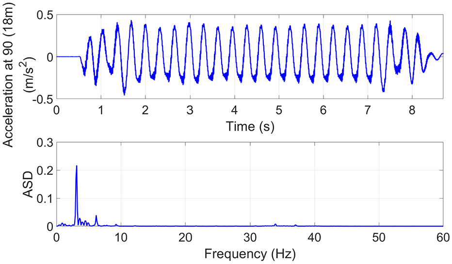
Model including a smooth track and TTBI.

Figure 9.

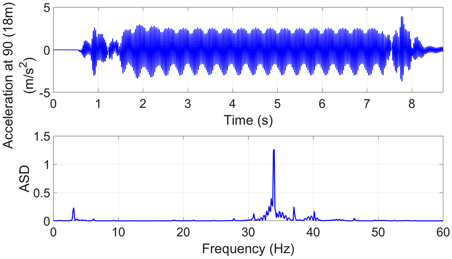
Model including a non-smooth track (i.e. a track with irregularities) and TTBI.

Since damage is typically a local phenomenon as already mentioned, it is reasonable to expect that the higher range of modal frequencies are contributing the most for damage detection, as these modes are more sensitive to local effects. The combination of filtered data and ANNs as an instrument for damage detection can be investigated for instance by using low- and high-pass filters to cut off the high- and low-frequency components of the bridge dynamics, respectively, and using separately each of the obtained trimmed signals to retrain and test the networks. The results attained from testing each trained network can be compared with the results from the original one (that uses unfiltered data), enabling to understand if the selected frequency range has indeed a significant effect in the learning of the ANNs. In particular, it is to be investigated if the consideration of the lower frequencies can be negligible when the data are obtained from measurements.

Now, it has been proven that the modal low-frequency data are not worthless per se in the damage detection process, as many studies have shown, including one by the authors of this article where the method is only validated with data obtained from a simplified FE model. If using measurements from a real structure or from a full model including TTBI that takes into consideration aspects such track irregularities, such as what is done in this article, it can be proven that the high-frequency data are better for damage detection in general. It remains to be stressed out again that the conclusion is valid for the method herein proposed and if low- and high-frequency data are both available, which will more likely happen when the system is to be deployed out in the field.

Case study I: numerical experiment

In this section, the methodology presented in the previous section is applied to a case study based on a numerical model of a bridge, developed with the intention of verifying the proposed approach. Main focus is put on the TTBI model and on the Mahalanobis distance as means for novelty detection (one class classification).

The bridge

The measurement of the dynamic response of bridges is a common procedure in the assessment of such complex structures. The type of excitation source–designated forced vibration can be used to excite the bridge by an external force, in this study activated by a crossing vehicle, which can produce high enough response amplitudes that can ease the interpretation of results. It is important to stress that the high-frequency content of the measured signal is forced vibration. This does not invalidate the method but is rather its strength: as mentioned before, it is difficult to excite and identify the high-frequency modes; however, using this method, one can avoid modal identification. There is enough information in the high-frequency forced vibration to successfully identify damage, as it will be shown in the “Results” subsection under the current section.

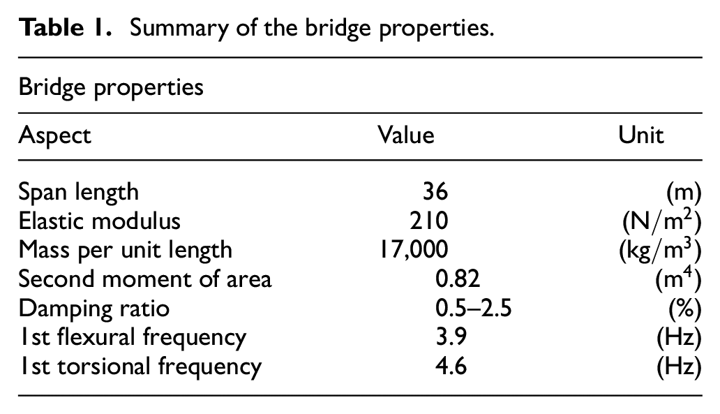
A case study is developed based on a 36-m long composite bridge located in the north of Sweden—the Skidträsk Bridge (Figure 10). The bridge consists of two simply supported steel beams and a concrete deck that carries a single ballasted railway track. The fundamental properties of the bridge are specified in Table 1, and additional aspects of the structure can be found in Cantero et al.¹⁸

Figure 10.

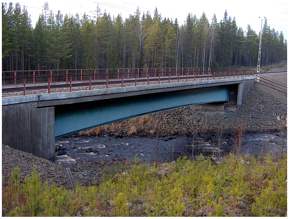
The Skidträsk Bridge.

Table 1.

Summary of the bridge properties.

Bridge properties
Aspect	Value	Unit
Span length	36	( $m$ )
Elastic modulus	210	( $N / m^{2}$ )
Mass per unit length	17,000	( $kg / m^{3}$ )
Second moment of area	0.82	( $m^{4}$ )
Damping ratio	0.5–2.5	(%)
1st flexural frequency	3.9	(Hz)
1st torsional frequency	4.6	(Hz)

The FE model

A 2D rigid contact model that includes the effects of TTBI is used in this study based on the previous work of Arvidsson,¹⁹ which enables to account for aspects such as track irregularities. The element size in the FE model is assumed to be 20 cm which, for a bridge length of 36 m, gives a total of 180 elements. The coupled equations of motions are solved by direct integration. Given the complexity and detail of the model, comprehensive description about its characteristics such as vehicle, track, beam, wheel–rail contact, profile definition, and so on are found in Arvidsson.¹⁹ Figure 11 shows a scheme of the TTBI model.

Figure 11.

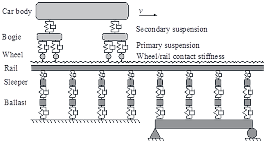
TTBI model. Different track models, vehicle models, and wheel–rail contact models can be chosen.

The Skidträsk Bridge is regularly subjected to the loading of two particular types of trains, a commuter passenger train and a freight train. For the purpose of this study, however, the real trains designed for the line are substituted by the universal train HSLM models, in particular HSLM-A1.

Model aspects and uncertainties

Throughout its life span, a structure will be subjected to more or less varying loads at the same time that the building materials naturally age. Such varying circumstances are propitious for the development of damage, which can compromise the structural safety, and thus need to be considered. In this article, hundreds of simulations of train passages over the bridge were performed under the following conditions:

The train type and bridge are the same over all the simulations that are carried out. This seeks to ensure that predictions are reliable as perceived changes in the response of the structure will not be due to changes in loading conditions;

The speed of the train changes within a certain range, from simulation to simulation (see subsection “Data collection” in the current section);

A healthy structure is considered in one version of the simulations (for training and testing of ANNs) but not in a second and posterior versions where different damage case (DC) scenarios are considered (for testing of ANNs);

Gaussian distributed white noise was posteriorly used to corrupt the acceleration time-histories straightly originated from the simulations.

Supplementary simulations were performed in order to have an overview of different settings and assumptions of the model and how those affect the results, namely the frequency spectrum of the structure’s response:

An irregular track is considered in one version of the simulations but not in a second version (Figures 8 and 9);

The TTBI is considered in one version of the simulations but not in a second version (Moving Force solution), both with irregular track (Figures 9 and 12).

Only the scenarios with irregular track and TTBI (Figure 8) are analyzed further in the case study given the aim of the article.

Figure 12.

Model including a non-smooth track (i.e. a track with irregularities) and Moving Force solution.

Data collection

Accelerations are recorded at selected locations—1, 2, and 3 in Figure 13. Choosing the sensor location is not a simple task but, reasonably, one could think that the points of the bridge that experience the largest response (e.g. displacements) should be the instrumented locations. For a simply supported bridge, the preferable points are at 1/4, 2/3, and 1/2 of the span length (Figure 13, sensors 1, 2, and 3, respectively).

Figure 13.

Bridge scheme: sensor locations (•) and damaged element ().

The sampling frequency with which the input data are given to the ANN, that is to say the time interval between two consecutive input data points, can affect the ANN’s performance. It may be so that the original sampling frequency is too high to acquire the information one needs. Sampling too fast and using the correspondent data to train an ANN may lead to the most accurate predictions but that is achieved at the expense of significantly time-consuming training periods. This suggests that in some cases it may be reasonable to down sample, so as to exclude redundant information. This is however dependent on the bridge and excitation method, hence it is important to look at the amplitude spectrum of the measured signals from which the training data are obtained. In this case, the computational time is quite reasonable even when the original sampling frequency is considered, and therefore the authors opted to provide input data to the ANN at such frequency. The sampling frequency is 1000 Hz, and the data are measured as long as the train is going over the bridge. A total of 250 trains traveling within a speed range described by the normal distribution $(μ, σ) = (200, 2)$ are observed and, for each, the acceleration time history is saved. Noise was posteriorly added to the generated acceleration time histories. After several simulation sets and by looking at the output signal, a noise simulation of 5% magnitude ended up being chosen.

In order to separate and obtain low- and high-frequency contents, a fourth-degree Butterworth filter is applied and the cut off frequency is set to be 20 Hz in reference to the amplitude spectrum of the measured signals obtained in a similar fashion to those in Figures 8, 9, and 12. 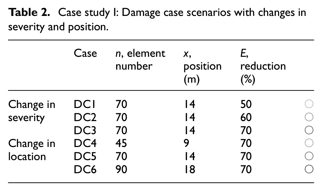The structural damage model is implemented as the reduction in a contribution to the element stiffness matrix equivalent to a scalar reduction of the elastic modulus ( $E$ ) of the material. In the context of the numerical model, this means decreasing the stiffness of the element closest to the chosen damage position. The damage extension can be adjusted without difficulty by reducing the stiffness of more elements.

Several local DC scenarios corresponding to different positions and magnitudes of damage are investigated as DC scenarios, shown in Table 2. Each DC is tried out independently noting that DC3 and DC5 are the same but used in two different groups—change in severity and change in location. Although a 50% reduction (and higher) in stiffness can appear exaggerated, this value is difficult to relate to because the extent is also important. These percentages are rather given as a qualitative description of damage and the minimum detectability of the method, also as a ground for comparison with alternative methods, falls outside the scope of this work.

Table 2.

Case study I: Damage case scenarios with changes in severity and position.

	Case	$n$ , element number	$x$ , position (m)	$E$ , reduction (%)
Change in severity	DC1	70	14	50
	DC2	70	14	60
	DC3	70	14	70
Change in location	DC4	45	9	70
	DC5	70	14	70
	DC6	90	18	70

The ANNs

There is no clear recipe for the optimal ANNs configuration, especially given the nature of problems that can be solved by this set of algorithms. Thus, it is key to train several networks while varying some aspect of their configuration and look at their performance, in order to understand which are the best settings.

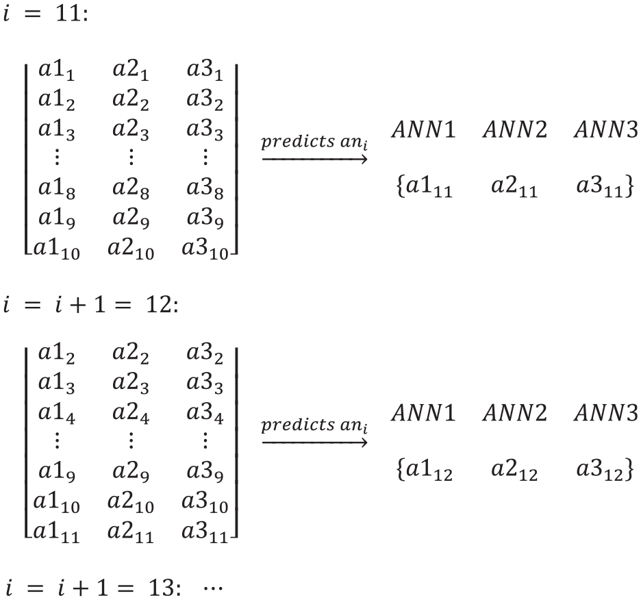
The Neural Network toolbox in MATLAB was used to apply the ANNs to the present case study. To predict the output, which is the current acceleration at one point of the structure coincidental with one sensor, the 10 previous accelerations of each sensor were used, meaning a total of $30 = 10 \times 3$ input neurons. As such, it is not the entire time series that is given as input but only a few discrete values in the vicinity of the point that the ANN is predicting. A sliding window method is applied to predict the following points of the time series dataset. One separate network was trained for each of the three sensors: the input matrix is the same for all but each predicts a different element of the output vector (Figure 14). In addition, it should be noted that while it is true that the predicted accelerations are not entirely dependent on the acceleration given as input, there is a strong correlation between them.¹⁴ It is this correlation than the ANN exploits.

Figure 14.

Case study I: input matrix and output vector for each time instant i. In $a n_{i}$ , $n$ stands for the sensor number (1, 2 or 3) and $i$ for the time instant.

As mentioned earlier, the optimal selection of the ANN training and architectural parameters can be an exhaustive process. Judging which input features (damage-sensitive) are relevant is an open problem as well. As such finding the optimal ANN model turns out to be a trial–error process which is case dependent. In this sense, limited number of configurations were tested and each was obtained from a different combination of parameters that have to be specified: the number of neurons in the hidden layer, the training algorithm, the amount of input data, and so on. The best configuration was considered to be the one that gives an optimal balance between the ANN’s ability to predict and the computational time required for training. Based on the results and for this case study, an ANN with eight hidden neurons was used. During the first attempts more neurons were used but that did not only increase tremendously the computing time as it did not yield any improvements in the network’s predicting accuracy. The training time with eight hidden neurons takes about one hour. The total amount of data sets is split into 170 and 50 for training and test, respectively. In turn, during the training phase the algorithm divides the data into training/validation/testing in the proportions 70%/15%/15%, respectively. The ANNs used are feed-forward neural networks,²⁰ and the training algorithm is the Levenberg–Marquardt backpropagation²¹ algorithm. Training is carried out according to trainlm with the parameters set to default values and hyperbolic tangent sigmoid as transfer function.

Results

The current section shows some of the relevant results obtained from the analysis of the case study.

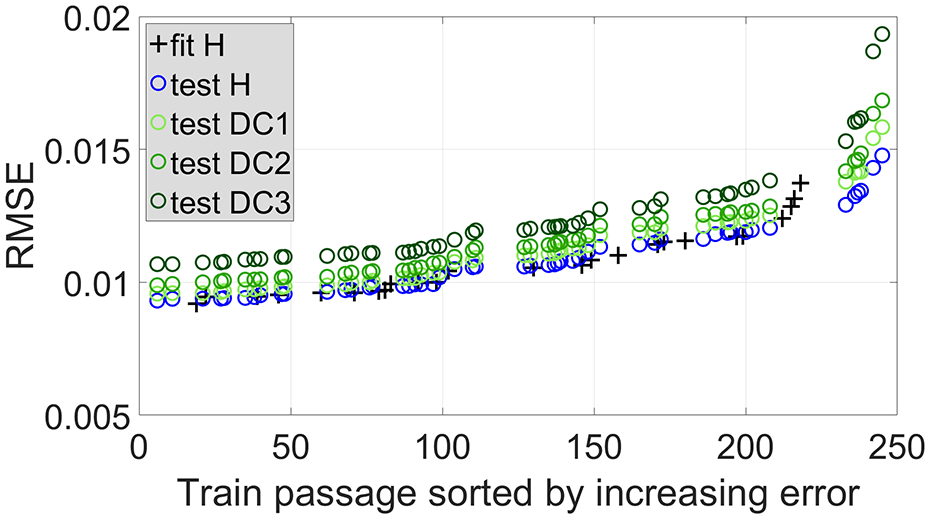
Different magnitudes and locations of damage were tried out according to Table 2. For example, looking at sensor 3 (at mid-span) and if unfiltered data are analyzed, testing the ANN with measured data from healthy (H) and DC1–DC3 gives rise to the prediction errors ( $m / s^{- 2}$ ) shown in Figures 15 and 16, ordered by increasing error or increasing train speed, respectively.

Figure 15.

Prediction error sorted by increasing error for sensor 3 and DC1–DC3.

Figure 16.

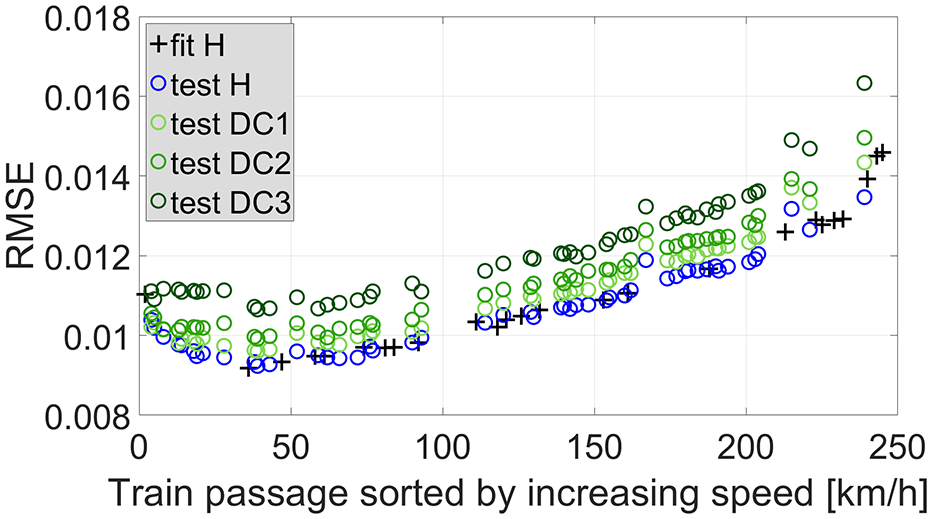
Prediction error sorted by increasing speed for sensor 3 and DC1–DC3.

An obvious separation is found between the prediction errors related with testing data for healthy () and damaged () conditions. The larger the damage, the larger the expected separation, which provides a first qualitative assessment of the damage severity.

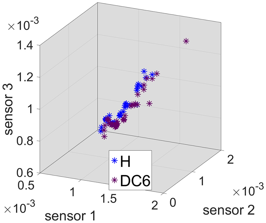
Figure 17 shows a three-dimensional plot of the prediction errors related with testing data for healthy () and DC6 () conditions and for each sensor (one per axis) with unfiltered data. The same plots for HPF (high-pass filter) and LPF (low-pass filter) data are shown in Figures 18 and 19, respectively.

Figure 17.

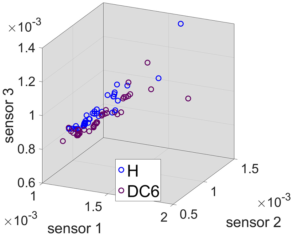
Prediction errors for all sensors: unfiltered data.

Figure 18.

Prediction errors for all sensors: HPF data.

Figure 19.

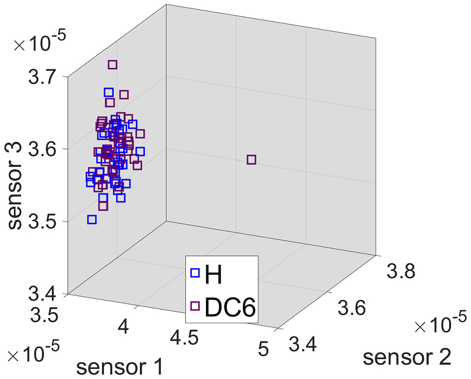
Prediction errors for all sensors: LPF data.

Two clouds of points corresponding to the two conditions are easily differentiable to the naked eye in the unfiltered and HPF cases, whereas for the LPF case the two clouds of points are indistinguishable. In fact, the separation between unfiltered and HPF is very similar, suggesting that, if given the unfiltered data, the algorithm will focus on the high frequency content, as expected.

This phenomenon can be verifiable through numbers. From the covariance matrix $(σ_{xy})$ of the reference distribution, one can obtain the correlation coefficient $(ρ_{xy})$ , which is a normalized measurement of how two variables in a data set are linearly related. When unfiltered data are used

{ρ_{xy}}^{U} = \frac{σ_{xy}}{σ_{x} σ_{y}} = [\begin{matrix} 1.0000 & 0.9113 & 0.9289 \\ 0.9113 & 1.0000 & 0.9776 \\ 0.9289 & 0.9776 & 1.0000 \end{matrix}]

(2)

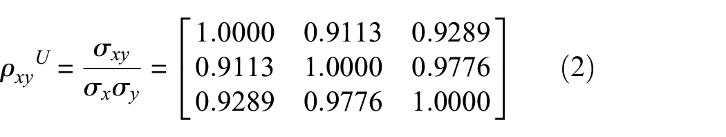
where a perfect correlation of each sensor with itself is evident, as well as a very strong positive correlation between different sensors.

The same happens when HPF data are used, with

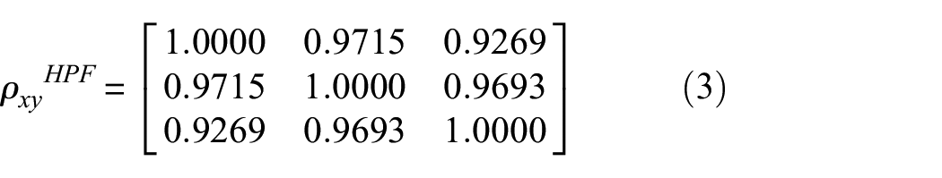
{ρ_{xy}}^{HPF} = [\begin{matrix} 1.0000 & 0.9715 & 0.9269 \\ 0.9715 & 1.0000 & 0.9693 \\ 0.9269 & 0.9693 & 1.0000 \end{matrix}]

(3)

However, when LPF data are used the correlations are noticeably non-existent as

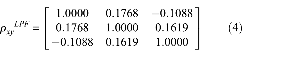
{ρ_{xy}}^{LPF} = [\begin{matrix} 1.0000 & 0.1768 & - 0.1088 \\ 0.1768 & 1.0000 & 0.1619 \\ - 0.1088 & 0.1619 & 1.0000 \end{matrix}]

(4)

Each sensor (or ANN) makes predictions for one specific point in the structure. To acquire more accurate information on the state of the structure, the information coming from all available sensors can be combined. As such, for each train passage, the prediction errors of sensors 1, 2, and 3 can be combined into one DI according to equation (1).

To better understand how the DIs turn out for each state of the structure, Figures 20 to 22 show the box plots regarding the DIs for DC4, DC5, and DC6, respectively, considering unfiltered, HPF, and LPF data. Box plots graphically display data through five measures: the extremes, the upper and lower hinges (quartiles), and the median. The spaces between the different parts of the box indicate the degree of dispersion and skewness in the data, and the individual points, falling outside the extremes, represent outliers. One of the advantages of this method is that it is nonparametric, meaning that it displays variations in samples of data without making any assumptions of the underlying statistical distribution.

Figure 20.

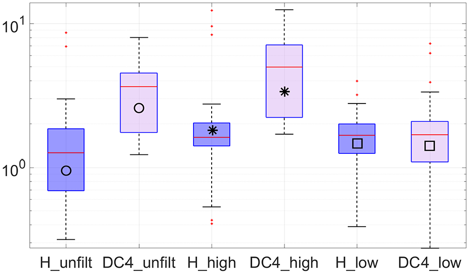
Unfiltered, HPF, and LPF boxplots of damage indexes associated with DC4 (y-axis in log-scale).

Figure 21.

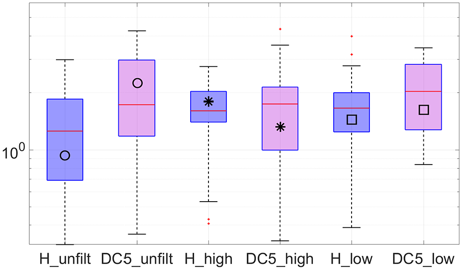
Unfiltered, HPF, and LPF boxplots of damage indexes associated with DC5 (y-axis in log-scale).

Figure 22.

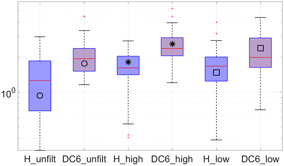
Unfiltered, HPF, and LPF boxplots of damage indexes associated with DC6 (y-axis in log-scale).

Looking at Figure 20, it is undeniable that healthy and DC4 states are hardly distinguishable from each other if LPF data (□) are used, implying that the system is not capable of detecting said damage. Contrarily, if HPF data (*) are used, said damage is easily identified as the healthy and damaged boxes do not even overlap. Similar detectability using HPF data is evident in Figure 22, regarding D6. In the light of DC5 (Figure 21), drawing conclusions about the preference of LPF data over HPF data for the purpose of damage detection is more vague.

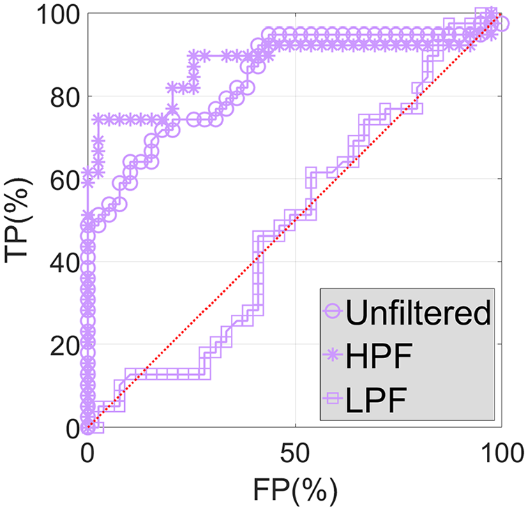
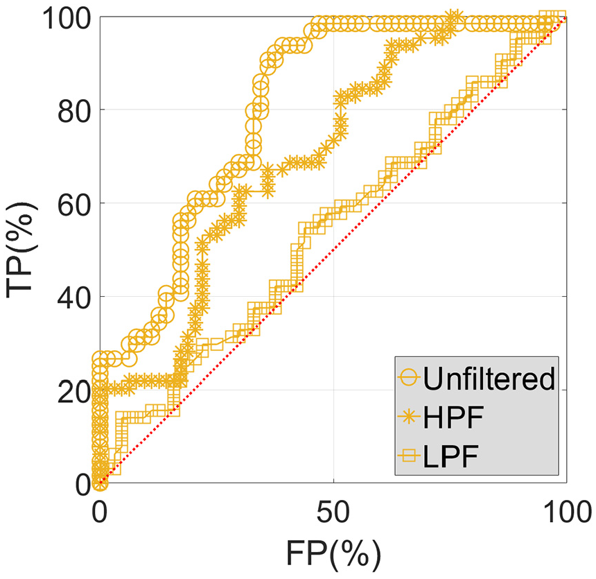
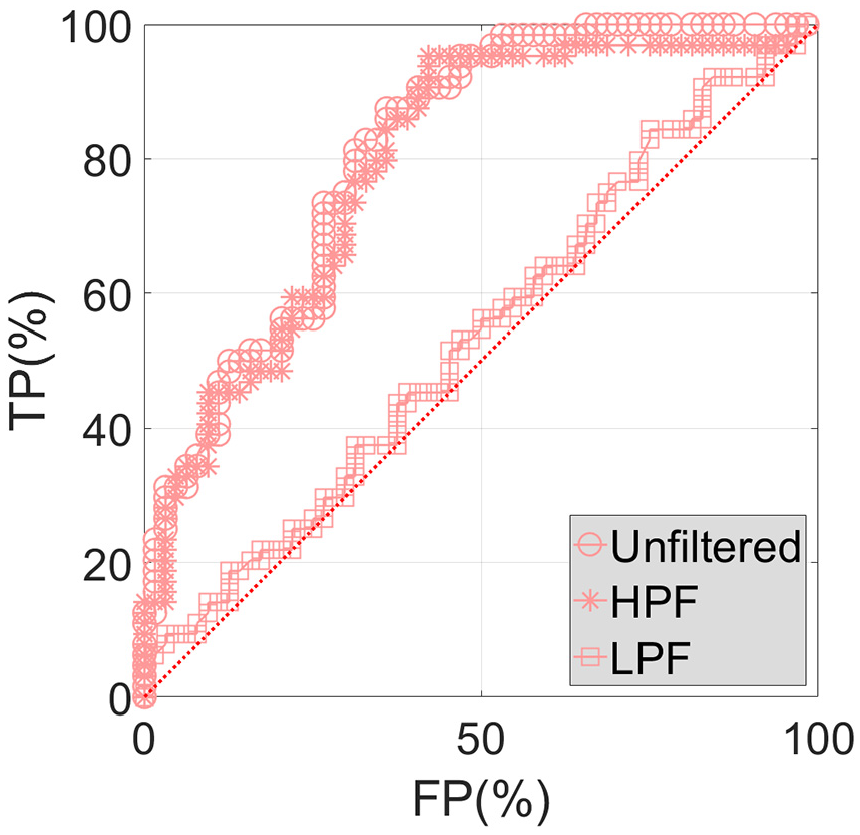
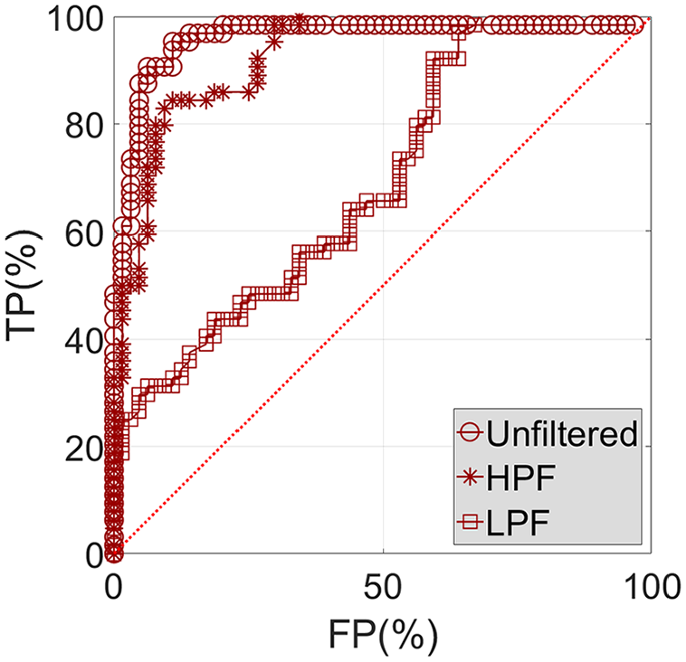
Based on a significant number of DIs (in this case 39) for which the diagnosis and the true condition is known (either healthy or damaged), ROC curve analysis can be used to determine the ability of the diagnostic test (the monitoring system) to predict the condition. Once calculated the prediction errors and thus DIs, detection thresholds of different magnitudes can be tried out. For each of these, a DI will either fall above or below, indicating positive or negative detection, respectively. As we know the true condition associated with each DI, we can label each detection instance as being a true or a false positive and the ROC curves can be created. Further description about ROC curves and the process to obtain them can be found in Neves.²² Figures 23 to 25 show the ROC curves associated with DC4, DC5, and DC6, respectively, considering unfiltered, HPF, and LPF data.

Figure 23.

Unfiltered, HPF, and LPF ROC curves associated with DC4.

Figure 24.

Unfiltered, HPF, and LPF ROC curves associated with DC5.

Figure 25.

Unfiltered, HPF, and LPF ROC curves associated with DC6.

In Figures 23 and 25, the ROC curves associated with unfiltered and HPF data are very similar to each other, while the ROC curve associated with LPF data are clearly separable, particularly in Figure 23. This shows the inferior ability of the system to perform damage detection based solely on LPF data.

Figure 24, which shows the ROC curves associated with DC5, is an example of how it is not always possible to demonstrate that HPF data are better than LPF data for the purpose of damage detection based on ANNs. Nonetheless, in the majority of the DC scenarios it is possible to verify precisely that, while the opposite (LPF data being better than HPF data) never occurs. This means that in the worst situation HPF and LPF data enable the damage detection system to perform with the same quality, although the tendency is for the former to do better than the latter.

Case study II: field experiment

In this section, the methodology presented in the “Methodology” section is applied to a case study based on measurements performed on an existing bridge, developed with the intention of verifying the proposed approach. Main focus is given to the ROC curves.

The bridge

The Old Lidingö Bridge (Figure 26) located in Stockholm, Sweden, was constructed between 1917 and 1925 and was initially designed to be used by pedestrians, road vehicles, and heavy freight trains. Due to the growing traffic demands, in 1971 road traffic was relocated to the newly built Lidingö Bridge and later, in 1978, freight train traffic was discontinued in the Old Bridge. At the moment, it carries one rail track that serves the light rail with a daily average of nine thousand travelers, as well as a pathway designated for pedestrians.

Figure 26.

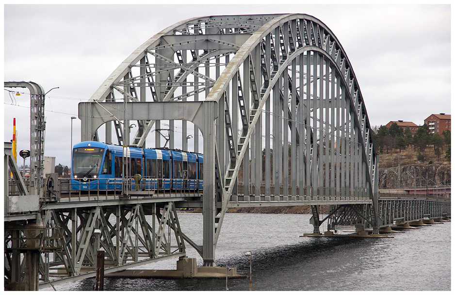
The Old Lidingö Bridge.

The Old Lidingö Bridge is a steel truss bridge with a total length of 740 m. With 140 m, the longest span consists of a riveted steel arch. The remaining spans are made of riveted steel trusses located below the deck and the end span on both sides is made of a grid of beams.

The bridge has been subject to considerable long periods of high loads induced by freight train traffic in the past, and it is well known that time-dependent degradation processes such as corrosion and fatigue can cause severe damage. Significant damage caused by fatigue has not been reported but severe corrosion (Figure 27) has been documented during the inspections. Other reported types of damage are missing rivets and bolts and defective bearings. A summary of the results of 2015 inspections is provided in Ahne.²³ According to the results of a measuring campaign performed in May 2012, reported in Karoumi,²⁴ unusual large movements had been noticed at support 6 during inspection of the bridge. That motivated in part the placement of sensors as described in the next section.

Figure 27.

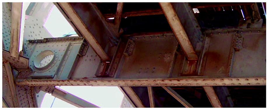
Heavily corroded crossbeam.

The monitoring system

The most recent ongoing measurements in the Old Lidingö Bridge are expected to enable the long-term monitoring of the structure’s condition, as well as to follow up the actual behavior at critical parts of the bridge. A wireless sensor network (WSN) system was installed, and the sensor locations are shown in Figure 28.

Figure 28.

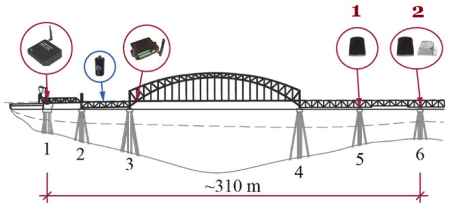
The wireless monitoring system.

In order to test the system’s performance and reliability, the number of sensors is intentionally limited in the system installed so far. The system configuration is however susceptible to adjustments and can be expanded according to necessity. Based on the outcome of previous inspections, the system consists at the moment of one node for strain measurements close to support 3, a total of three nodes for acceleration measurements in supports 5 and 6, and one inclinometer at support 6. A gateway for data aggregation is located at support 1, and the energy harvesting device is located in the span between supports 2 and 3. A gateway of type WSDA-1500-LXRS for data aggregation is located at support 1. The node for strain measurement close to support 3 is of type V-Link-200 with four channels for uniaxial strain gauges. At support 5, one accelerometer node of type GLink-200 is located. Support 6 is instrumented with two accelerometers, one G-Link-2G and one GLink-200, and one inclinometer of type SST440 connected to the WSN through a V-Link-200. All parts of the WSN are delivered from the company LORD MicroStrain Sensing Systems. More detailed information about the sensors can be found in Leander et al.²⁵

Data collection

Data have been continuously collected by the WSN system since September 2017. Daily measurements are performed during three periods of the day: around 8 a.m., 12 a.m., and 12 p.m., the latter corresponding to a period where there is no traffic on the bridge. Contrasting with the previous numerical case study, reality is much more complex and it may be imperative to account for operational and environmental variability when designing a response-based damage detection system. If the monitoring is meant to be performed continuously and structural states over very different seasons are meant to be assessed and compared with the reference state, it is important that the training data cover a large span of time. That should enable the system to account for temperature fluctuations over the year when making predictions regarding the response of the structure. Alternatively, a narrower time interval may be used for training the ANN, if one can ensure that the predictions to be made will fall in a time interval with similar temperatures of that used for training the ANN. The sampling frequency of the signal is 64 Hz. This sampling frequency is significantly lower than the one used in the previous case study due to limitations of the monitoring setup in the Old Lidingö Bridge. For a wireless system, reducing the sampling rate allows to extend the service life of the batteries as far as possible and above 64 Hz the power consumption increases quite fast.²⁶ In the present study, only the data of the two triaxial accelerometers—sensors 1 and 2—placed in supports 5 and 6 respectively (Figure 28), were considered for the analysis, in particular vertical accelerations. In order to separate and obtain low- and high-frequency contents, a fourth-degree Butterworth filter is applied and the cut off frequency is set to be 6.4 Hz in reference to the amplitude spectrum of the measured signals obtained in a similar fashion to those in Figures 8, 9, and 12.

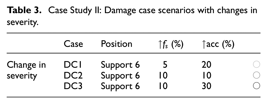
Measurement data corresponding to damaged scenario were created to test and validate the damage detection algorithm. Since the condition of the bridge did not change during the monitoring campaign, the damage is introduced artificially into data from the reference state. This is done by simulating a loss of stiffness in one of the monitored supports that would lead to an increase in the vibration amplitude and a reduction in the frequencies present in the signal. The increased amplitude (↑acc) is achieved by multiplying the signal by a fixed factor. The reduction in the frequencies of the signal is achieved by re-sampling the data to a higher frequency↑ $f_{s}$ ), thus shifting all the frequencies present in the signal by a fixed factor.

Several DC scenarios (Table 3) are tested: in all cases, damage is assumed to be located at support 6, but the damage severity varies from case to case.

Table 3.

Case Study II: Damage case scenarios with changes in severity.

	Case	Position	↑ $f_{s}$ (%)	↑acc (%)
Change in severity	DC1	Support 6	5	20
	DC2	Support 6	10	10
	DC3	Support 6	10	30

The ANNs

Once more, the Neural Network toolbox in MATLAB was used. In this case study, both input and output data comprise, just like in the first case study, acceleration measurements: the former consists of the past acceleration data from both the sensors, and the latter consists of the current acceleration at one of the two sensors. Similarly to what happens in the previous case study, the ANN configuration here chosen is the product of an empirical process. The 10 previous accelerations of each sensor were used, meaning a total of $20 = 10 \times 2$ input neurons (Figure 29). One single network was trained to predict for sensor 2 at support 6 and, for that ANN, 20 hidden neurons were used. The total amount of available data sets, spreading over several months (September 2017–March 2018) with fluctuations of air temperature between 18°C and –13°C, is split into 200 and 65 for training and test, respectively. In turn, during the training phase the algorithm divides the data into training/validation/testing in the proportions 70%/15%/15%, respectively. The ANNs used are feed-forward neural networks and the training algorithm is the Levenberg–Marquardt backpropagation algorithm. Training is carried out according to trainlm with the parameters set to default values and hyperbolic tangent sigmoid as transfer function.

Figure 29.

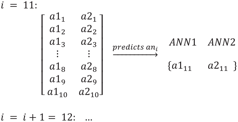
Case study II: input matrix and output vector for each time instant i. In $a n_{i}$ , $n$ stands for the sensor number (1, 2) and $i$ for the time instant.

Results

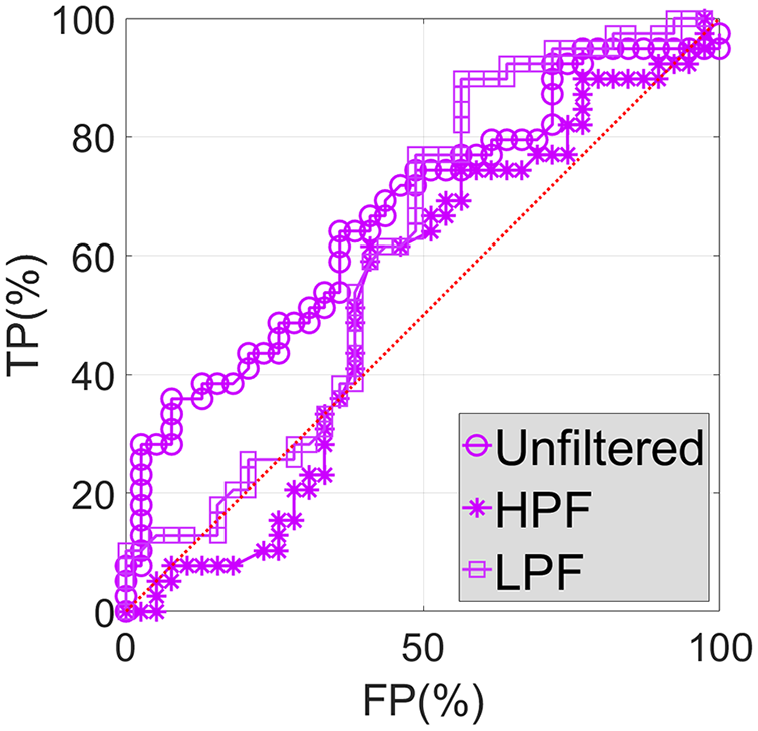
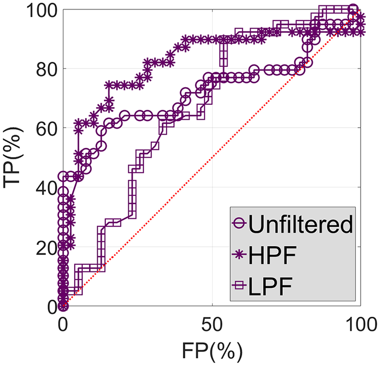
Based on a significant number of DIs (in this case from 65 data samples) for which the diagnosis and the true condition is known (either healthy or damaged), the ROC curve can be used to determine the ability of the diagnostic test (the monitoring system) to predict the true condition. Figures 30 to 32 show the ROC curves associated with DC1, DC2, and DC3, respectively, considering unfiltered, HPF, and LPF data.

Figure 30.

Unfiltered, HPF, and LPF ROC curves associated with DC1.

Figure 31.

Unfiltered, HPF, and LPF ROC curves associated with DC2.

Figure 32.

Unfiltered, HPF, and LPF ROC curves associated with DC3.

As expected DC3, as the most severe DC, is associated with the best ROC curves (Figure 32). In particular, the curve concerning the unfiltered data is an almost perfect ROC curve (this exhibits an inverted L shape). While all curves tend to improve with the severity of damage, it is notorious that the ROC curves concerning LPF data are quite unsatisfactory in all studied cases. This first important conclusion means that providing such data to the system that performs damage detection leads to poor results, with detection being made with nearly 50% accuracy: an instance, independently of its true condition (healthy or damage), has equal probability of being correctly or incorrectly labeled. This is clearly shown in Figures 30 and 31, where the ROC curve respecting LPF data is practically depicted as 45-degree line. The second important conclusion to retain is that the ROC curve pertaining the HPF data is quite similar to the one pertaining the unfiltered data, as anticipated. Following the latter conclusion, it is important to note that even though the use of unfiltered data is sufficient, and thus adding an extra step for filtering is unnecessary, the main idea to retain by showing this graphs is, in any case, that the accuracy of the ANN is coming mainly from the high-frequency part.

Conclusion and future research

A method for SHM and damage detection supported by machine learning is proposed in this article. In light of two case studies, numerical and experimental, the proposed method was implemented and validated. It was shown that the method is sufficiently robust when performing novelty detection (one-class classification), even in the presence of noisy measurements. When looking at the frequency domain, the presence of damage appears to have the largest effect in the higher frequencies of the spectrum, suggesting that damage detection based on characteristic features of the structure may be more efficient when applied to data measurements originated from high-frequency forced vibrations. The verification of this hypothesis was executed by trying out ANNs trained with different data sets associated with just low-frequency or just high-frequency data or both. Several conclusions can be made based on the attained results:

The Mahalanobis distance is a helpful tool to bring together the information from all sensors that constitute the monitoring system. The collected information can be articulated into a single value—a DI—representative of the condition of the monitored structure;

The numerical experiment case study showed that the correlation coefficients between the sensors are remarkably low for LPF data and significantly high for HPF data (and unfiltered data). This could suggest that a damage detection system making use of such sensors will barely take any advantage of the use of multiple sensors as the information by them provided individually cannot be integrated.

The numerical experiment case study showed through boxplots that, overall, the HPF data used alone for both training and testing is mainly responsible for the accuracy in damage detection when compared with LPF data;

The field experiment case study showed that with increasing damage severity, the respective ROC curves (unfiltered, LPF, and HPF) seem to improve. Such improvement is higher for unfiltered and HPF ROC curves, whereas it is minimal for the LPF ROC curve. This is an undeniable indication that the algorithm will focus on the high-frequency content if unfiltered data are provided.

The most valuable outcome of this article, albeit limited to the proposed ANN-based method, is that the focus on high-frequency acceleration response for the purpose of SHM, more particularly intended for damage detection, deserves further investigation.

Furthermore, none of the case studies aims at validating the ability to find real damages or quantify the damage states. However, they can be called validations considering the ability to detect anomalies in the response of the structure. With this objective in mind and in light of two case studies of different nature, the proposed method has shown to work. The authors suggest thus that it would be interesting to apply the proposed approach to other existing bridges. It could be one where for example, even given the unavailability of damaged data, some sort of intervention (e.g. repair) has taken place and where monitoring data are available both before and after said intervention. This would allow to comprehend how smaller degrees of change in the behavior of the monitored structure would affect the ability of the method for novelty or damage detection. Moreover, ascertaining what is the smallest damage that makes successful detection possible is desirable in order to determine the sensitivity of the method. This would certainly add value and increase the credibility of the proposed ANN-based approach for damage detection.

Footnotes

Funding

The author(s) received no financial support for the research, authorship, and/or publication of this article.

ORCID iD

Ana C Neves

References

Italy bridge collapse: what might have caused it? BBC, August 2018, https://www.bbc.com/news/world-europe-45188668

Doebling

Farrar

Prime

, et al. Damage identification and health monitoring of structural and mechanical systems from changes in their vibration characteristics: a literature review. Shock Vib Digest 1996; 30(2): 91–105.

Khoa

NLD

Alamdari

Rakotoarivelo

, et al. Structural health monitoring using machine learning techniques and domain knowledge based features. In: Zhou

Chen

(eds) Human and machine learning. Human–computer interaction series. Cham: Springer, 2018, pp. 409–435.

Heckman

. Damage detection in civil structures using high-frequency seismograms. Pasadena, CA: California Institute of Technology, 2013.

Yan

Chen

. Structural health monitoring using high-frequency electromechanical impedance signatures. Adv Civil Eng 2010; 2010: 429148.

Farrar

Worden

. Structural health monitoring: a machine learning perspective. Chichester: John Wiley & Sons, 2013.

Rytter

. Vibration based inspection of civil engineering structures. PhD Thesis, Aalborg University, Aalborg, 1993.

Farrar

Doebling

Nix

. Vibration-based structural damage identification. Phil Trans Math Phys Eng Sci 2001; 359(1778): 131–149.

Carden

Fanning

. Vibration based condition monitoring: a review. Struct Health Monit 2004; 3(4): 355–377.

10.

Casas

Moughty

. Bridge damage detection based on vibration data: past and new developments. Front Built Environ 2017; 3: 4.

11.

Bhuiyan

Bao

Poddar

, et al. Toward identifying crack-length-related resonances in acoustic emission waveforms for structural health monitoring applications. Struct Health Monit 2017; 17(3): 577–585.

12.

Moll

Kathol

Fritzen

, et al. Open guided waves: online platform for ultrasonic guided wave measurements. Struct Health Monit 2019; 18: 1903–1914.

13.

Tsang

. Condition-based maintenance: tools and decision making. J Qual Mainten Eng 1995; 1(3): 3–17.

14.

Neves

Gonzalez

Leander

, et al. Structural health monitoring of bridges: a model-free ANN-based approach to damage detection. J Civil Struct Health Monit 2017; 7(3): 689–702.

15.

Swingler

. Applying neural networks: a practical guide. London: Academic Press, 1996.

16.

Yeager

Gregory

Key

, et al. On using robust Mahalanobis distance estimations for feature discrimination in a damage detection scenario. Struct Health Monit 2019; 18(1): 245–253.

17.

Benítez

Castro

Requena

. Are artificial neural networks black boxes? IEEE Trans Neural Network 1997; 8(5): 1156–1164.

18.

Cantero

Ülker-Kaustell

Karoumi

. Time–frequency analysis of railway bridge response in forced vibration. Mech Syst Signal Process 2016; 76–77: 518–530.

19.

Arvidsson

. Train–track–bridge interaction for the analysis of railway bridges and train running safety. Stockholm: KTH Royal Institute of Technology, 2018.

20.

Schmidhuber

. Deep learning in neural networks: an overview. Neural Network 2015; 61: 85–117.

21.

Press

Teukolsky

Vetterling

, et al. Numerical recipes in C. Cambridge: Cambridge University Press, 1992.

22.

Neves

. Structural health monitoring of bridges: model-free damage detection method using machine learning. Stockholm: KTH Royal Institute of Technology, 2017.

23.

Ahne

. Sammanfattning av 2015 års inspektioner—Gamla Lidingöbron. Rapport 2015—12—03 [Summary of the 2015 inspections—Old Lidingö Bridge. Report 2015-12-03]. Stockholm: Grontmij Anläggningsunderhåll, 2015.

24.

Karoumi

. Gamla Lidingöbron: Fördjupad analys av mätta accelerationer på fundament 6 och 8 [Old Lidingö Bridge: comprehensive analysis of measured accelerations on foundations 6 and 8]. Stockholm: KTH Byggvetenskap, 2012.

25.

Leander

Karoumi

Rohner

, et al. Smart condition assessment, surveillance and management of critical bridges. In: 1st international conference on health monitoring of civil & maritime structures (HeaMES), London, 2018.

26.

https://s3.amazonaws.com/download.microstrain.com/Power+Profiles/G-Link-200+power+profile+v12_43124/G-Link-200+power+profile+v12_43124.htm

The influence of frequency content on the performance of artificial neural network–based damage detection systems tested on numerical and experimental bridge data

Abstract

Keywords

Introduction

Damage detection using SHM

Methods for damage detection

Signal processing and filtering

Methodology

ANNs

Performance of the method for damage detection

The frequency range of the signal

Case study I: numerical experiment

The bridge

The FE model

Model aspects and uncertainties

Data collection

The ANNs

Results

Case study II: field experiment

The bridge

The monitoring system

Data collection

The ANNs

Results

Conclusion and future research

Footnotes

Funding

ORCID iD

References