
Abstract
Wheel condition assessment is of great significance to ensure the operation safety of trains and metro systems. This study is intended to develop a Bayesian probabilistic method for online and quantitative assessment of railway wheel conditions using track-side strain-monitoring data. The proposed method is a fully data-driven, nonparametric approach without the need of a physical model. To enable defect identification using only response measurement, the measured dynamic strain responses of rail tracks during the passage of trains are processed to elicit the normalized cumulative distribution function values representative of the effect of individual wheels, which in conjunction with the frequency points are used to formulate a probabilistic reference model in terms of sparse Bayesian learning. Through cleverly realizing sparsity by introducing hyper-parameters and their priors, the sparse Bayesian learning makes the resulting model to exempt from overfitting and generalize well on unseen data. Only the monitoring data in healthy state are needed in formulating the reference model. A novel Bayesian null hypothesis significance testing in terms of scale-invariant intrinsic Bayes factor, which does not suffer from the Jeffreys–Lindley paradox, is then pursued in the presence of new monitoring data collected from possibly defective wheel(s) to detect wheel defects and quantitatively assess wheel condition. The proposed method in fully Bayesian inference framework is verified by utilizing the real-world monitoring data acquired by a distributed fiber Bragg grating–based track-side monitoring system and comparing with the offline inspection results.
Keywords
Introduction
Passenger safety is the highest priority in mass transportation. This is especially true in modern high-speed rails in view of their mass transportation volume and fast speed. If a high-speed train runs in failure, it will result in a disastrous loss of mass lives and rail infrastructure. The current rail operation control systems do not have the functions of online detection of structural health and real-time response to potential structural failure, since in the current practice structural faults or damage are detected offline in depots or maintenance yards at scheduled time intervals. However, structural faults may occur during in-service operation; this issue is especially important for the high-speed trains that are in a high frequency of services. In this regard, development of effective online structural fault diagnosis methods is a core focus for preventing catastrophic failure as well as prolonging the service life of high-speed rails.
Wheel condition assessment is of great importance to ensure railway safety and to reduce the maintenance cost of railway infrastructure. Wheel defects because of wheel out-of-roundness, such as wheel flats, wheel shells, and wheel polygonization, can induce damage to both train and rail track, trimming down safety and ride comfort of in-service trains and increasing operation and maintenance costs for railway system.1–3 Early detection of wheel condition and timely re-profiling or replacement of defective wheels confer great benefits in railway safety and economy. During the past several decades, offline inspection and online monitoring techniques have been proposed for wheel condition assessment. Incipient offline inspection measures wheel profiles at workshop by contact-type measurement devices together with visual inspections. 3 The inspection procedure is often costly in time and must be performed on a maintenance schedule. More time-effective ways are using noncontact-type measurement devices such as ultrasonic waves.4,5 Online monitoring techniques allow detection to be conducted in real time, aided by various sensing technologies such as piezoelectric accelerators,6–9 piezoelectric strain gauges,10–12 fiber Bragg grating (FBG) sensors,13–15 acoustic emission sensors, 16 and laser sensors.17,18 The online monitoring techniques for rail system are categorized into onboard monitoring and track-side monitoring in accordance with the deployment of sensors. Onboard monitoring installs sensors on in-service trains, that is, particularly useful to monitor the deterioration of rail infrastructure such as rail track defects,19–21 rail fasteners,22,23 and rail irregularities. 24 The track-side monitoring6,7,10–18 installs sensors on tracks or surrounding areas, with the purpose of detecting the condition of in-service trains including wheel qualities.
Apart from various monitoring techniques, diagnosis and prognosis algorithms are at the core of research to realize precise wheel condition assessment. Belotti et al. 7 explored high-frequency wavelet coefficient maxima from vertical accelerations of rails as an indicator of wheel flats. Jia and Dhanasekar 8 investigated local wavelet energy average from vertical accelerations of bogies for identifying wheel flats. Based on wheel impact load detector, Stratman et al. 10 proposed the maximum dynamic ratio (MDR) for wheel condition assessment. The MDR is defined as the ratio of maximum dynamic impact loads to static axle loads, and its value of 3 has been adopted as a threshold for flawed wheels in European Union. 12 In line with an FBG-based track-side monitoring system, Wei et al. 13 defined a wheel condition index that is linearly proportional to the averaged strain alterations of rail bending but inversely proportional to train speed. Filograno et al. 14 suggested that a 70% increase in strain energy of rail bending with respect to noise levels is a good measure of significant wheel defects. However, the aforementioned deterministic diagnostic algorithms are incapable of dealing with the uncertainties resulting from measurement of noise or error and randomness in wheel–rail interactions. Statistical models are deemed to achieve more reliable and persuasive diagnostic results. 25
Statistical approaches have recently been developed for wheel condition assessment. Skarlatos et al. 6 attempted to establish a fuzzy-logic model for undamaged wheels by correlating maximum acceleration amplitudes with nominal train speeds and 1/3-octave bands from 80 Hz to 5 kHz. The statistical hypothesis test was conducted to investigate the probability of existence of wheel flats and the damage extents. Krummenacher et al. 12 proposed two automatic detection algorithms for wheel defects by means of machine learning methods. One algorithm employed support vector machine to learn and classify wavelet features extracted from the wheel impact load monitoring data, and the other automatically learned the original monitoring data and classified wheel conditions using deep artificial neural networks. The proposed methods could achieve at least 10% improvement in identifying wheel defects in comparison with the MDR, but defect extents were not identifiable. Liu and Ni 15 assumed a Gaussian distribution for the normalized rail bending strain and employed the Chauvenet’s criterion to signal wheel defects. Zhang et al. 9 proposed a Bayesian dynamic linear approach for modeling ride quality evolution due to deteriorating wheel qualities and for probabilistic assessments of wheel condition with the use of onboard monitoring data of acceleration acquired from the running train.
This article aims to develop a Bayesian machine learning approach for online wheel condition detection using the track-side strain-monitoring data. The proposed method features the following merits: (a) it uses only the dynamic strain responses of tracks collected during the passage of trains; (b) it is fully data-driven and requires only the monitoring data collected in healthy state in formulating the reference model; (c) by means of sparse Bayesian learning (SBL), the built probabilistic reference model exempts from overfitting and bears favorable generalization ability due to sparsity embedded by SBL; and (d) the proposed method accounts for uncertainties arising from measurement and modeling errors. Toward the above, the Fourier amplitude spectra (FASs) of the measured track dynamic strain responses in healthy state are obtained to elicit normalized cumulative density functions (CDFs) that characterize the patterns of healthy wheels. The CDFs together with the corresponding frequency points are then used as outputs (response variables) and inputs (explanatory variables) to train a probabilistic reference model by means of SBL.26,27 There exist various sources of uncertainties in the measured track dynamic strain response data such as measurement noise and variability in the stochastic wheel-rail dynamics. The SBL allows the uncertainties arising from measurement and modeling errors to be accounted for in the model formulation. More importantly, through introducing hyper-parameters and sparsity-inducing priors, the SBL elicits a probabilistic regression model exempting from overfitting in terms of highly sparse representation. When new monitoring data on track dynamic strain responses coming from the effect of a possibly defective wheel are made available, the discrimination between the new measurements and the model predictions is evaluated in terms of an intrinsic Bayes factor (IBF) for defect detection and quantification. The IBF is derived through Bayesian null hypothesis significance testing (BNHST) which does not suffer from the Jeffreys–Lindley paradox.
The remainder of this article is organized as follows. Section “Feature extraction through track-side monitoring” describes the feature extraction from raw measurement data acquired by an FBG-based track-side monitoring system. Section “Model formulation by SBL” describes the formulation of a probabilistic reference model by means of SBL. Section “Bayesian hypothesis testing for wheel defect detection” delineates the detection of wheel defects and quantitative assessment of wheel condition by BNHST and scale-invariant IBF. Finally, section “Conclusion” gives the conclusions drawn.
Feature extraction through track-side monitoring
Track-side monitoring system
As illustrated in Figure 1, the FBG-based track-side monitoring system for this study consists of two arrays of FBG strain sensors deployed on two parallel tracks of a rail segment, two optical cables, a high-speed optical interrogator, and a desktop or notebook computer. To facilitate the detection of minor wheel defects, the sensors are densely deployed along rail length but the instrumentation needs just to cover a range of rail slightly longer than the wheel perimeter. The FBG sensors are connected through optical cables to a high-speed optical interrogator which is controlled by a computer for data acquisition and processing. Both the interrogator and the computer can be located far away from the instrumented rail to facilitate remote monitoring.
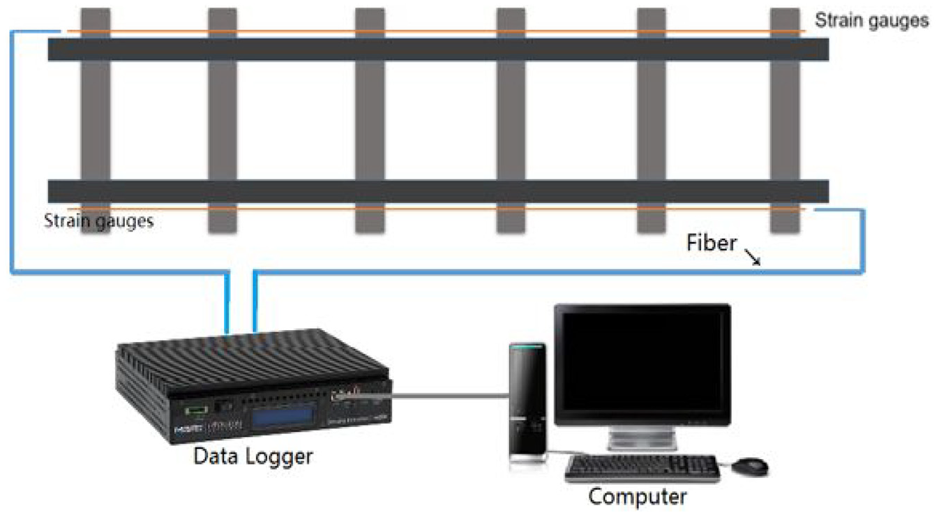
Track-side monitoring system using distributed FBG strain sensors.
Figure 2 shows the deployment of the track-side monitoring system on an in-service rail. In this implementation, each sensor array comprises 21 FBG gauges evenly spaced at 0.15 m intervals on rail foot of each single track, and the total instrumentation range reaches 3.0 m to enable the sensing of rolling action of the whole circumference of the wheel tread (the diameter of wheel is 0.92 m). Both the optical interrogator and the computer are operated in an auxiliary office which is about 120 m away from the monitoring area. The FBG sensors have been calibrated in laboratory before their installation to obtain strain sensitivity and temperature sensitivity, but in general the temperature compensation is not necessary as the time for online monitoring of the passage of a whole train just lasts for a few seconds, during which the environmental temperature does not change dramatically. The wheel-rail rolling friction may cause heating and cooling effects on the top surface of the rail, such that, the rail temperature varies to some extent, but such effects mainly influence the area of rail head and are less significant in rail foot.28,29 When both FBG strain gauges and temperature sensors are deployed, it is easy to compensate the effect of varying temperature by subtracting from the measured strain a thermal-induced ingredient which is equal to a constant coefficient times the difference between the measured instant temperature and the recorded temperature at the installation of the sensor. 30
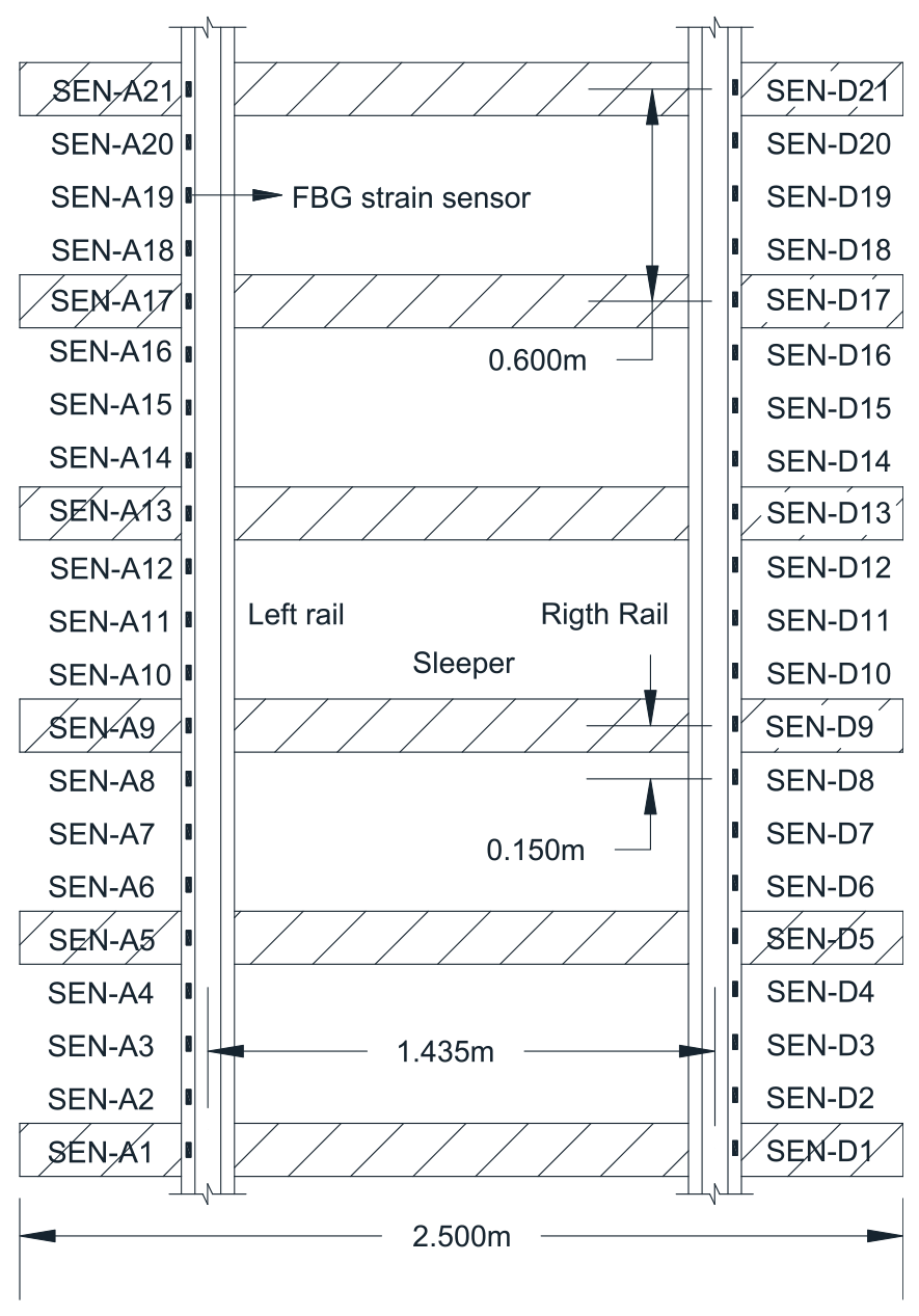
Deployment of FBG sensors.
Figure 3 illustrates the time history of longitudinal (bending) strain at rail foot monitored by the FBG sensor SEN-D2 (refer to Figure 2) when a typical eight-car passenger train passes through the instrumented rail at a nominal speed of 10 km/h. The sampling frequency
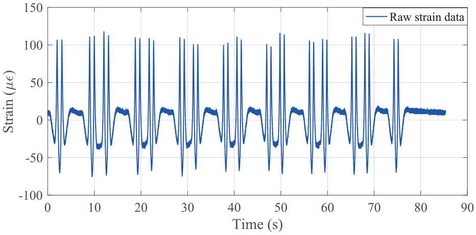
Rail foot strain recorded by SEN-D2.
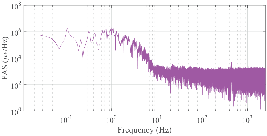
FAS of rail foot strain recorded by SEN-D2.
Data pre-processing
To obtain the information relevant to wheel quality, Filograno et al. 14 proposed an empirical formula to extract the wheel-sensitive response ingredients from rail strain-monitoring data, which is

where
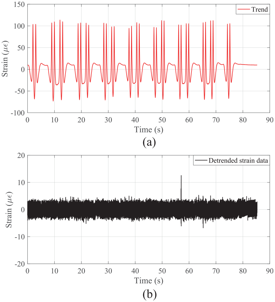
Rail strain recorded by SEN-D2: (a) trend response components containing frequencies lower than
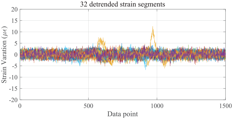
32 detrended datasets extracted from rail strain recorded by SEN-D2.
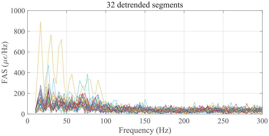
FASs of 32 detrended datasets recorded by SEN-D2.
Feature extraction
After obtaining the FAS, its values
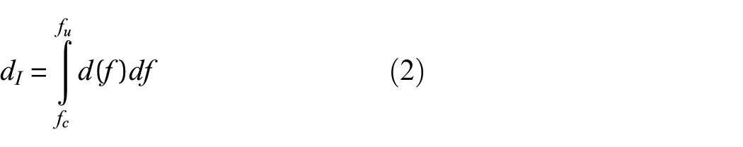
When a discrete Fourier transform (DFT) is employed,
where
where
The values of CDF range between 0 and 1 in
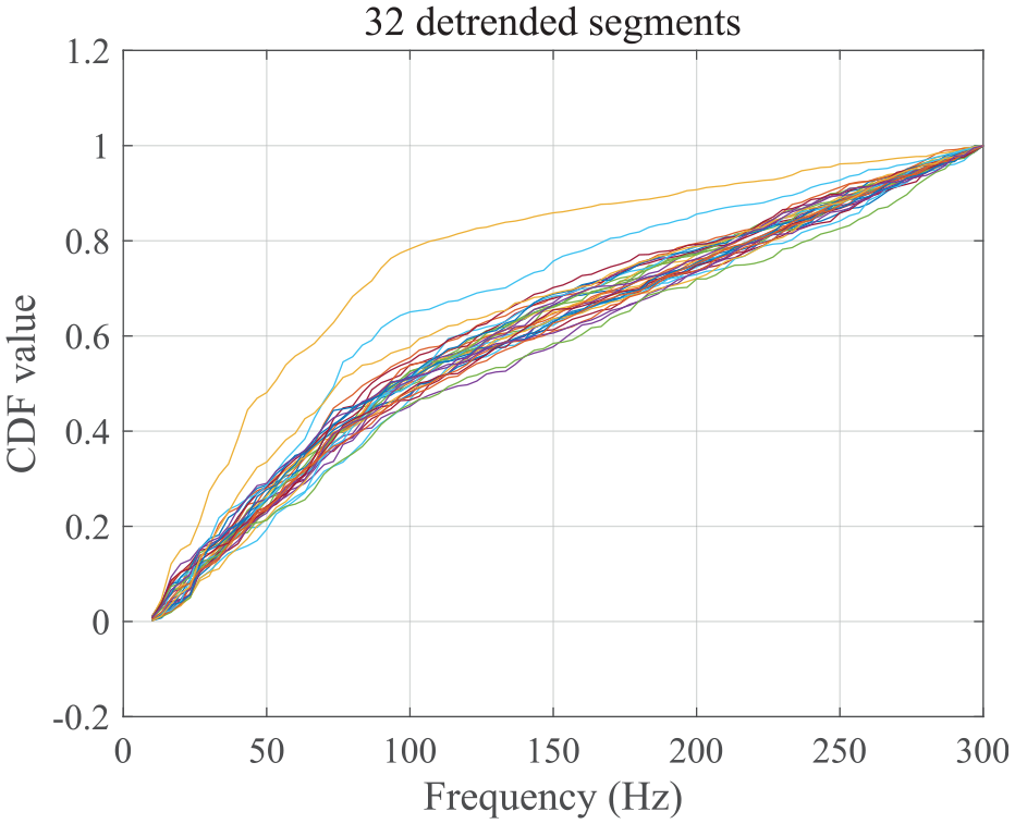
CDFs for normalized FASs of 32 detrended datasets recorded by SEN-D2.
Model formulation by SBL
SBL
SBL26,27 is a nonparametric machine learning approach that shares characteristics in common with support vector machine,
32
but produces probabilistic model outputs with dramatically few basis functions. Its ability of sparse representation and accurate prediction is primarily due to the Bayesian setting where uncertainty is taken into consideration and “inactive” basis terms can be automatically pruned through introducing hyper-parameters in the prior distributions of weight parameters (sparsity-inducing priors).
33
As a result, the SBL exempts from the problem of overfitting which often occurs in classical least-squares and penalized least-squares. Due to the above merits, there has been an increasing interest in the application of SBL for structural health monitoring (SHM).34–38 The basic theory of SBL for regression analysis is briefly introduced below. Given a dataset of input–output pairs

A nonparametric approach for modeling
where
where
where
and the prior for the noise level
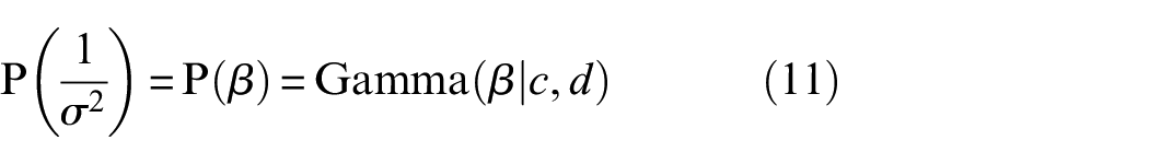
where

with the gamma function
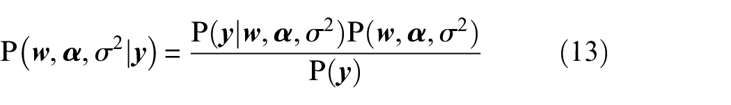
Typically, it is difficult to compute the joint posterior

where
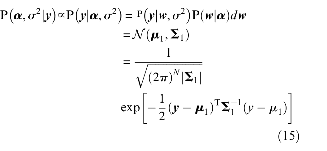
where


with
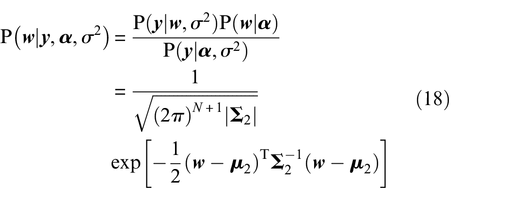
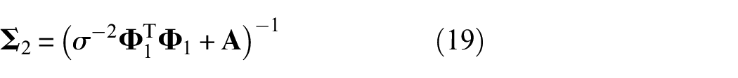
where the posterior covariance and mean vector for the weights are, respectively, given as

Given the most-plausible point estimators
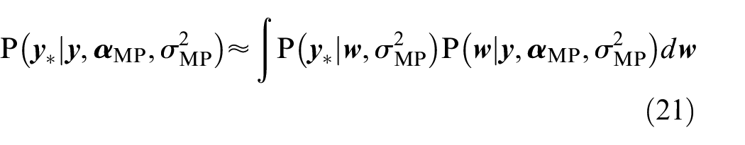
where
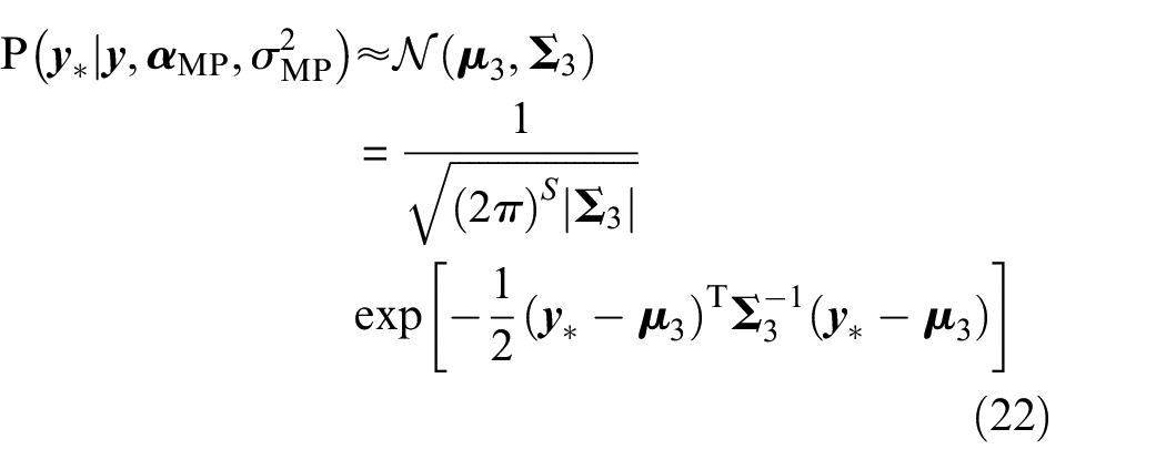
with


where
Implementation for model learning
In general, monitoring data at the model training stage is lopsided: it is prodigal in healthy state, but niggard (even null) in defective state. Wheel defects are diverse in type and extent, and monitoring data from defective wheels of each type can be very limited. By contrast, data for healthy wheels are often abundant. In the worst case where undamaged data are also not available, it is necessary to resort to a precise and validated physical model such as a high-fidelity wheel–rail interaction model and the method is no longer free of model. This study is intended to develop a nonparametric reference model using only the monitoring data from healthy wheels in the training phase, with which defective wheels can be identified in the testing phase. To help account for uncertainties arising from different sources, this model is established in a probabilistic framework by means of SBL. In this section, the monitoring data acquired by the sensor SEN-D2 as described in the preceding section are taken as an example to illustrate the model training by SBL and this process can be easily applied to other sensors.
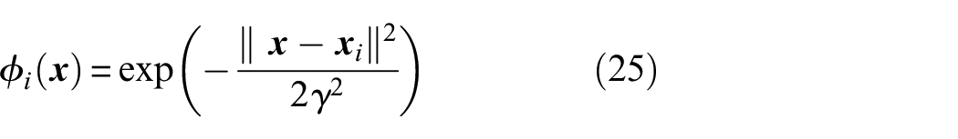
The monitoring data of rail foot strain response acquired by the sensor SEN-D2 contain the information about all 32 wheels (refer to Figure 3). The sequence of data is then separated and filtered to obtain the detrended datasets (Figure 6), their FASs (Figure 7), and normalized CDFs (Figure 8) stemming from individual wheels. The probabilistic model is trained in terms of SBL using the normalized CDFs which are elicited from the data collected by the sensor SEN-D2 during multiple trips of the train with all the wheels being in healthy state. Because of good adaptability, the Gaussian kernels are employed in this study as basis functions, given by
where
where
where
where
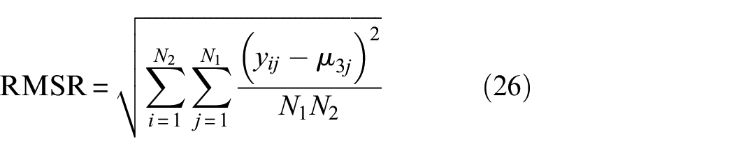
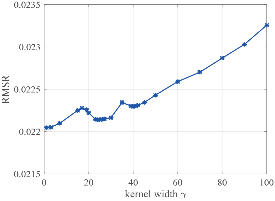
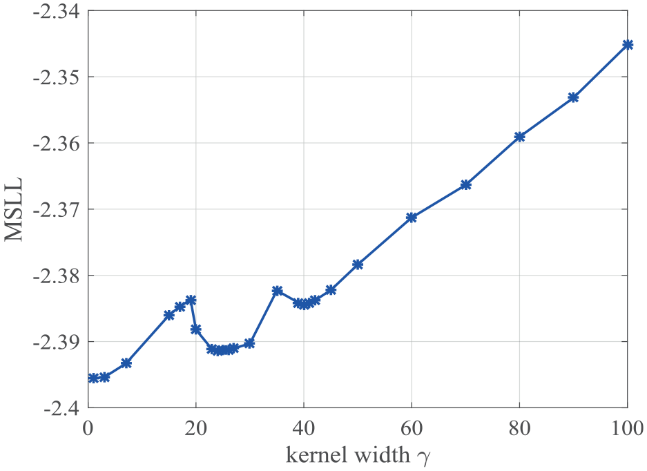
Then, SBL model is trained by successively increasing the kernel width
Model training with different kernel widths: (a)
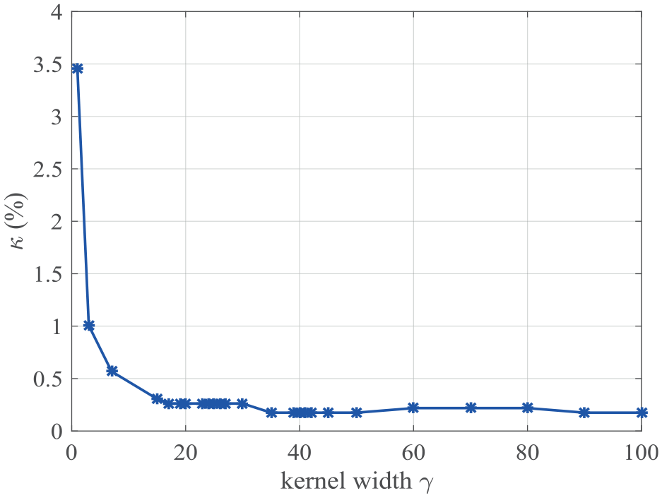
Sparsity ratio
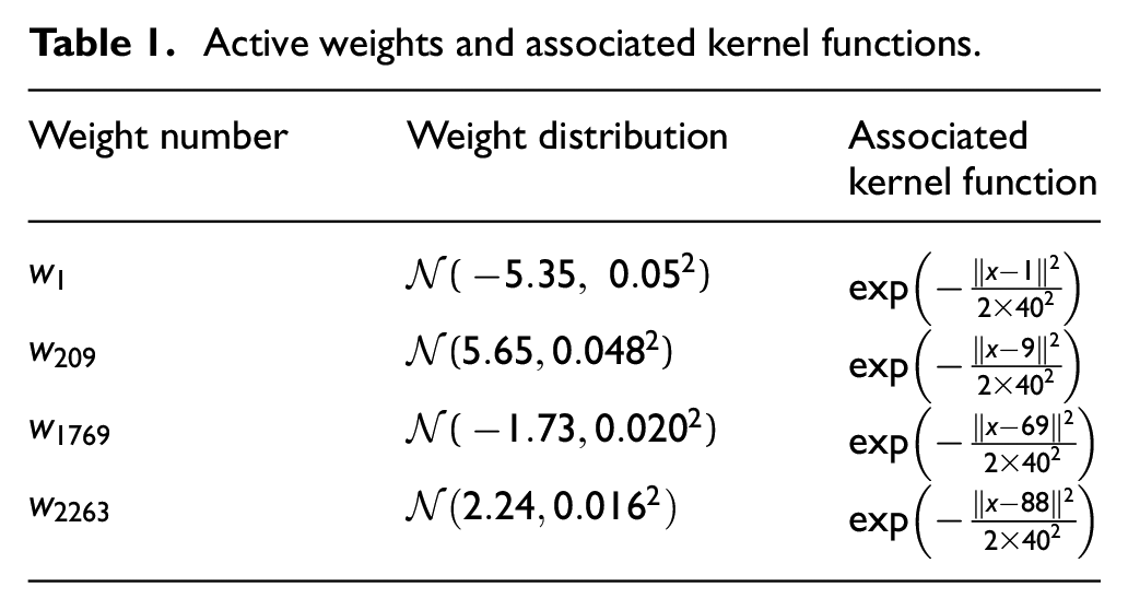
Active weights and associated kernel functions.
To validate the benefit of the SBL framework, a comparative study is conducted using the non-sparse Bayesian generalized linear (BGL) 40 model to learn the same training data. Table 2 provides a comparison between the SBL and the BGL models in terms of three performance indices. It is seen that while the learning performance in terms of RMSR and MSLL is comparable between the SBL and the BGL models, the SBL model utilizes dramatically fewer basis functions (much lower sparsity ratio), giving rise to a much simpler probabilistic model with stronger prediction ability.
Performance comparison of SBL and BGL models.
SBL: sparse Bayesian learning; BGL: Bayesian generalized linear; RMSR: root mean square residual; MSLL: mean standardized log loss.
In this study, the SBL model is formulated using the data collected under the nominal running speed of 10 km/h. This is due to the fact that the track-side monitoring system is often installed at a location immediately before trains arrive at a railway station or terminal, for the ease of operation, management, and maintenance. As a result, it allows both low-speed trains and high-speed trains to pass the monitoring area at a fixed speed. Certainly, the SBL model can be adaptive to a wide range of running speeds by incorporating an extra variable (train speed) in the basis functions in equation (25) if enough data covering different train speeds are available.
The formulated model is deemed to be robust to loading conditions as the loading conditions, such as fully loaded and non-loaded trains, do not significantly influence the wheel defect-incurred impact on the railway track, which has been validated by both numerical modeling 41 and field test. 1 Environmental conditions, such as wet track, ice, debris, and extremely temperature, may affect the pattern of wheel–rail interaction. To ensure the reliability of defect detection results by the proposed method, it is preferable to collect the monitoring data in the testing phase under the similar environmental conditions as to obtain the training data.
The model does not evolve with time because it is formulated to represent the initial defect-free state of railway wheels. If new monitoring data collected later are confirmed from healthy state as well, the model can be refined using the newly collected data as explained in the following section. In principle, the model does not need to be updated over time. Instead, the model can be utilized to investigate the deterioration of wheel condition over time.
Bayesian hypothesis testing for wheel defect detection
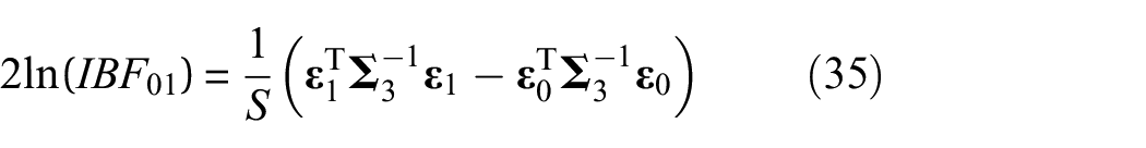
A variety of diagnostic criteria are available for damage or fault identification and quantification. In recognizing the shortcomings of the commonly used distance-based diagnostic methods, statistical hypothesis tests have gained growing interest in SHM applications. For example, Bayesian point null hypothesis testing (BPNHT) has been attempted for damage or fault identification and quantification in terms of Bayes factor.40,42,43 It is more robust than the distance-based diagnostic methods in that its resulting risk is averaged over the priors for unknown parameters in the hypotheses. However, the BPNHT is sensitive to the priors of the unknown parameters, giving rise to the so-called Jeffreys–Lindley paradox. In this study, we introduce a novel damage diagnostic logic in terms of BNHST and IBF, which does not suffer from the Jeffreys–Lindley paradox and the effect of sample size (data scale).
BNHST
In the previous section, a probabilistic model has been formulated by SBL using monitoring data in the state of healthy wheels. This model characterizes the stochastic CDFs in healthy state. Thus, a null hypothesis


where
where
where

Kass and Raftery
46
suggested interpreting
where
As identical Gaussian kernels are used in the model trained by SBL, the predicted uncertainties can be approximated by
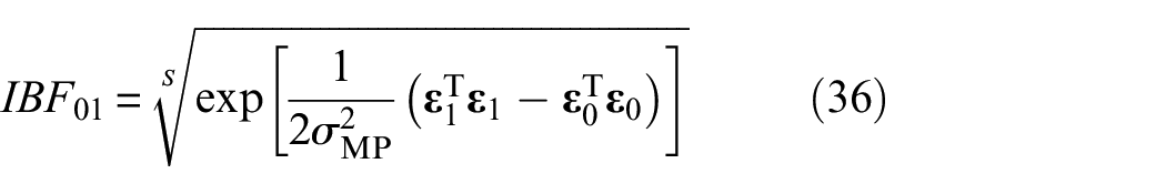
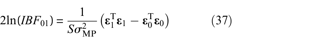
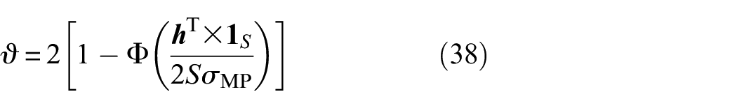
Accordingly, the false-positive diagnostic risk
When new monitoring data from potentially defective wheel(s) are made available, the predicted expectations
If the new monitoring data are confirmed from healthy state, the newly collected data can be used to update or refine the current SBL model by taking the joint posterior distribution
In comparison with the new defect-sensitive features characterized by the SBL model, the raw defect-sensitive features cannot be directly adopted to perform Bayesian hypothesis significance testing in the presence of new monitoring data because their uncertainties are not quantified. Moreover, the raw and the new features have different feature inputs and thus they are not directly comparable.
Diagnostic results of wheel defects using a single sensor
A blind test was later conducted by replacing some healthy wheels by defective wheels and running the train equipped with defective wheels on the rail instrumented with the track-side monitoring system. It provides in-situ monitoring data to verify the proposed wheel defect detection method. Moreover, after the blind test, the suspected defective wheels have been delivered to a workshop for offline wheel radius deviation measurement. As such, a comparison between the online diagnostic results by the proposed method and the offline inspection results can be made. It is worth noting that the monitoring data collected by a single sensor might be unable to capture the defect-relevant information in case the minor defective tread (e.g. a small flat) did not roll over the rail section deployed with the sensor; it would result in a false negative if using only the data from the single sensor. When using the monitoring data from all the deployed sensors, more reliable defect detection results would be obtained because the effect of minor defective tread must be sensed by at least one sensor if the sensors are densely deployed along a rail segment longer than the wheel perimeter. In the following section, both the wheel defect detection results using the monitoring data from a single sensor (SEN-D2) and from all the sensors are presented.
In the implementation of the proposed method, the shift parameters are set to be
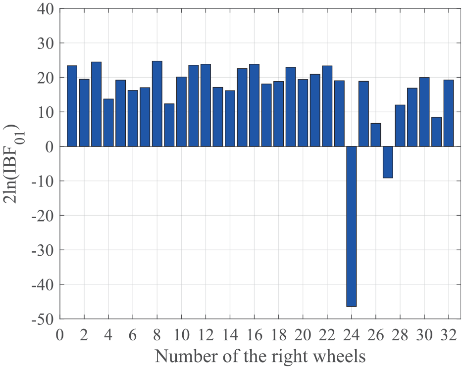
Condition assessment of right wheels using monitoring data from SEN-D2 deployed on right rail track.
Diagnostic results of wheel defects by integrating all sensors
The wheel defect detection is then pursued using the monitoring data from all sensors deployed on one side of the rail. As we are interested in finding defective wheels, the smallest IBF is used in the assessment, which is given by

where
Figure 14 provides the diagnostic results on the condition of the right wheels using the monitoring data from all 21 sensors deployed on the right rail track. It can be seen that the IBFs associated with the 1st, 6th, 24th, 27th, and 31st right wheels are negative, suggesting that the five wheels are potentially defective with different degrees. The 24th wheel is most heavily defective, while the 31st wheel is most weakly defective. With IBFs being positive, the other right wheels are diagnosed as healthy. By comparing Figure 14 with Figure 13, it is found that using only the monitoring data from the sensor SEN-D2 fails to identify the defects on the 1st, 6th, and 31st right wheels, while the results from the two settings indicate defects on the 24th and 27th wheels.
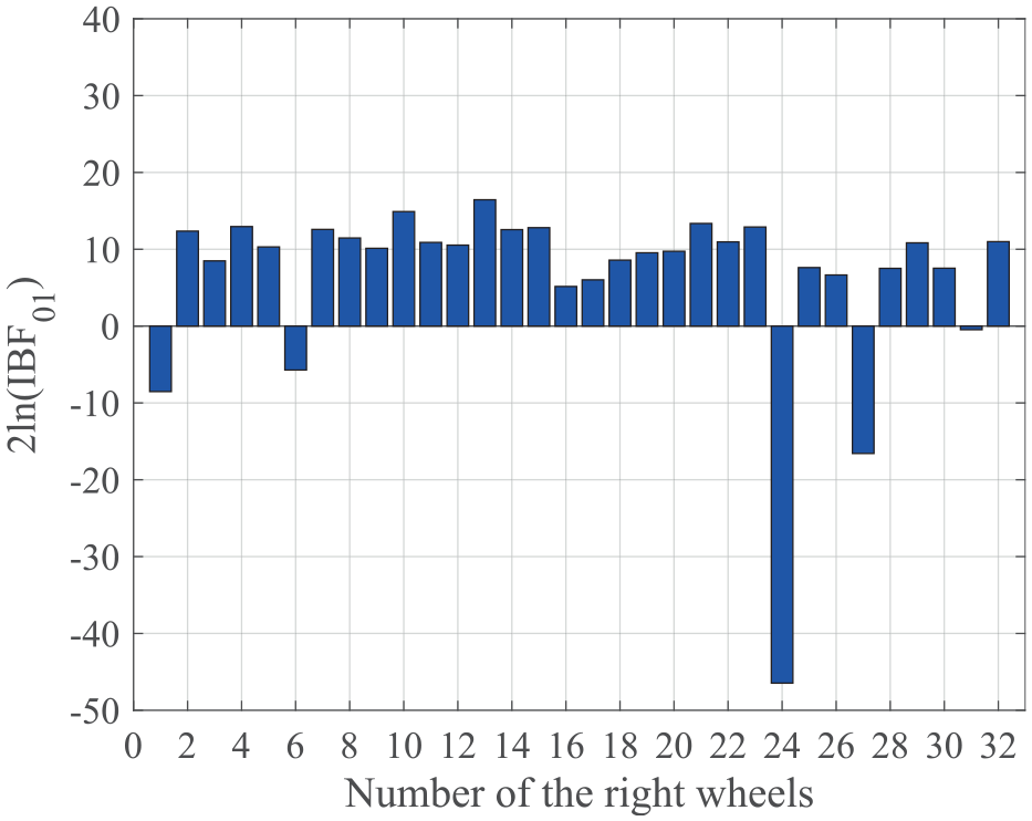
Condition assessment of right wheels using monitoring data from all sensors deployed on right rail track.
Figure 15 illustrates the diagnostic results on the condition of the left wheels when using the monitoring data from all 21 sensors deployed on the left rail track. It is observed that the IBFs for the 1st, 6th, and 27th wheels are negative, indicating that the three wheels are defective with the 27th wheel being most heavily defective. The other left wheels are diagnosed as healthy. The values of IBFs provide a quantitative measure to assess the degree of wheel defects. Smaller values of IBF indicate in general worse wheel conditions.
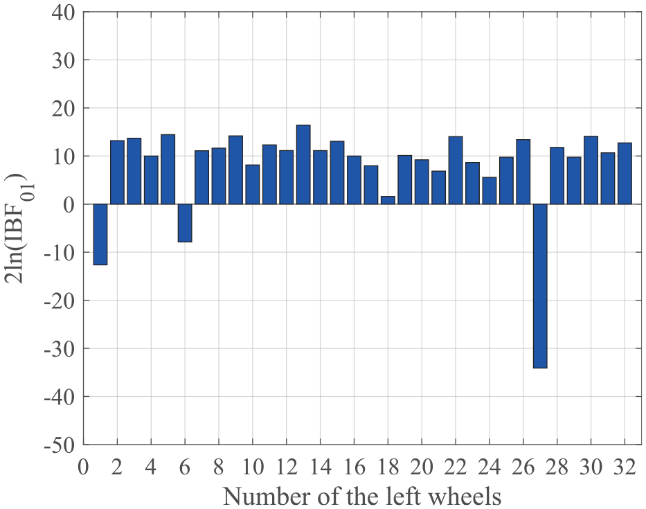
Condition assessment of left wheels using monitoring data from all sensors deployed on left rail track.
To validate the diagnostic results by the proposed online method, offline inspection on the suspected defective wheels was conducted afterwards in a workshop. The offline wheel radius deviation measurement indicates that the 1st, 6th, 24th, and 27th right wheels, and the 1st, 6th, and 27th left wheels are indeed defective, with large flats found on the 24th (36.0 mm in length), 27th right wheel (26.9 mm), and the 27th left wheel (34.6 mm). Although the 31st right wheel is diagnosed as weakly defective by the proposed method, it is in fact healthy. This warns us of the diagnostic risk imposed by the proposed method. Overall, the diagnostic results by the proposed online method are in good agreement with the offline measurement results.
Conclusion
A Bayesian machine learning approach for online detection of wheel defects and condition has been proposed in this study. With the aid of an FBG-based track-side monitoring system, CDFs for the normalized FASs of rail foot strain responses in the healthy state of wheels are extracted as characteristic features to train a probabilistic reference model by SBL. In the Bayesian probabilistic framework, the formulated model can account for uncertainties arising from the monitoring data (e.g. measurement noise and variability in the stochastic wheel–rail dynamics) and modeling error, and the SBL enables the model to perform well in either characterizing the training data or predicting unseen data. Because only a few basis functions are involved in the model, its computational efficiency is quite competitive especially on prediction, enabling fast diagnosis in wheel condition assessment. The diagnostic logic in terms of BNHST and scale-invariant IBF allows the unsupervised defect detection to be executed in a fully probabilistic inference context, ranging from the probabilistic model development in the training phase to the wheel defect diagnosis in the testing phase.
The proposed method is verified using the in-situ monitoring data acquired by a track-side monitoring system during the passage of a train with all wheels being healthy and with some wheels being defective, respectively, and is validated through comparing the diagnostic results obtained by the proposed online method and by the offline wheel radius deviation measurement. It turns out the following findings: (a) when using CDFs as characteristic features, a sparse representation of the probabilistic model containing only a few basis functions (four Gaussian kernels in the case of the optimal kernel width
Footnotes
Funding
The author(s) disclosed receipt of the following financial support for the research, authorship, and/or publication of this article: The work described in this paper was supported by a grant from the Research Grants Council of the Hong Kong Special Administrative Region, China (grant no. PolyU 152014/18E). The authors would also like to appreciate the funding support by the Innovation and Technology Commission of Hong Kong SAR Government to the Hong Kong Branch of Chinese National Rail Transit Electrification and Automation Engineering Technology Research Center (grant no. K-BBY1).