Validation of a procedure for the evaluation of the performance of an installed structural health monitoring system

Abstract

Validation of the performance of guided wave structural health monitoring systems is vital if they are to be widely deployed; testing the damage detection ability of a system by introducing different types of damage at varying locations is very costly and cannot be performed on a system in operation. Estimating the damage detection ability of a system solely by numerical simulations is not possible as complex environmental effects cannot be accounted for. In this study, a methodology was tested and verified that uses finite element simulations to superimpose defect signals onto measurements collected from a defect-free structure. These signals are acquired from the structure of interest under varying environmental and operational conditions for an initial monitoring period. Measurements collected in a previous blind trial of an L-shaped pipe section, onto which a number of corrosion-like defects were introduced, were utilised during this investigation. The growth of three of these defects was replicated using finite element analysis and the simulated reflections were superimposed onto signals collected on the defect-free test pipe. The signal changes and limits of reliable detection predicted from the synthetic defect reflections superimposed on the measurements from the undamaged complex structure agreed well with the changes due to real damage measured on the same structure. This methodology is of great value for any structural health monitoring system as it allows for the minimum detectable defect size to be estimated for specific geometries and damage locations in a quick and efficient manner without the need for multiple test structures while accounting for environmental variations.

Introduction

Low-frequency guided wave inspection allows for the rapid full-volume screening of tens of metres of pipework from a single inspection position. ¹ During an inspection, a wave pulse is induced into the pipe via a ring of piezoelectric ² or magnetostrictive^3,4 transducers attached to its outer wall. Changes in the cross-sectional area of the pipe wall will cause part of the propagating guided wave to be reflected.^5,6 These thickness changes can be caused by a number of benign features such as welds and pipe supports or by the growth of defects produced by corrosion or erosion. Reflected signals are recorded by the transducer ring such that, using the propagation time and reflection amplitude, the axial position and approximate cross-sectional area (CSA) change of the reflector can be determined.

In the framework most commonly used in industrial applications of guided wave screening of pipelines, a single collection is made with a detachable transducer ring. The measurement is subsequently interpreted manually by an inspector and defect locations determined. This approach is very time-consuming, and the inspection sensitivity and the probability of detection of a defect are dependent on the skill and experience of the individual operators. Repeated access to a pipe section is also highly costly, and therefore, there has been strong interest in advancing from the standard single inspection guided wave measurements to a structural health monitoring (SHM) system permanently installed on site, thus allowing for the continuous collection and interpretation of data. It was shown that such an SHM system based on an independent component analysis (ICA) algorithm^7,8 will allow for defects as small as 0.5%–1% cross-sectional area loss to be identified ⁹ reliably. This corresponds to an improvement in the minimum detectable defect size by a factor of around 5 compared to standard single inspection investigations. Guided wave SHM systems using piezoelectric transducers have also been investigated for structures other than pipes such as aircraft parts.^10,11

The purpose of this article is to evaluate the validity of a methodology used to assess the performance of a given SHM system regardless of the specific signal processing procedure employed. The methodology will be exemplified using an ICA-based SHM procedure as this was utilised by the authors in a previously conducted blind trial. ⁹ The authors appreciate that a large body of work exists on different methods of damage evaluation; however, a full discussion of this would distract from the purpose of this article. The reader is, however, encouraged to review other signal processing methods which have been investigated, for example, Gaussian mixture models.^10–13

Knowledge of the damage detection ability of a health monitoring system is of great importance to an operator as it allows for an informed statement to be made about the maximum size of defect that could be missed. For standard guided wave inspection, the minimum detectable defect size of the system is best estimated from the average noise level of a collection. This allows the operator to determine the detection threshold, which is usually set to be about twice the amplitude of the noise. This is not an appropriate approach for a health monitoring system as the smallest detectable defect signals can be below the noise level of the individual measurement.

The determination of the damage detection ability of a health monitoring system has a multitude of challenges. First, the probability of detection of the system is not solely determined by the equipment and the SHM procedure but also by the general condition of the pipe, as well as the environmental changes it undergoes during monitoring. Second, the false alarm rate is also of great concern in monitoring applications as the costs of following up defect indications can be substantial. The receiver operating characteristic (ROC) curve ¹⁴ is a valuable performance metric as it plots the probability of detection against the probability of false alarm. Unfortunately, determining the ROC curve for an SHM system is even more difficult than for a non-destructive testing (NDT) inspection system. This is due to the fact that the effect of environmental variations and potential transducer/instrumentation drift over a long period, as well as the changes due to damage of different types and severity at different locations, must be evaluated. This would involve an impractical number of test structures in the operational environment and an extensive programme of damage introduction over a long period. The environmental and operational conditions of the SHM system will also vary between different structures, thus causing results obtained from one setup not necessarily being transferable to others.

Another approach is to simulate the received signal; modern computational resources mean that it is relatively straightforward to reliably predict the signature produced by damage in guided wave measurements, even when it has a complex shape. ⁵ However, reliable prediction of signal changes due to environmental and other variability is much more difficult; on the other hand, obtaining experimental data with environmental variation on an undamaged structure is easy. Liu et al. ¹⁴ proposed a methodology of measuring data over multiple environmental cycles on an undamaged structure and synthetically adding damage to the resulting signals; this approach enables the addition of damage at different locations with different growth patterns and the investigation of other practical parameters such as the extent of environmental changes, damage severity and frequency of readings. They illustrated the approach of the guided wave monitoring of a single length of pipe in the laboratory with simple, flat-bottom hole defects.

The performance prediction methodology introduced by Liu et al. can be of great value for any kind of SHM system which collects frequent data. Since the damage detection ability of an installed health monitoring system depends not only on the measurement equipment used but also on the general state of the inspected structure, its geometry and the extent of environmental variations, the minimum defect size detectable in practice is difficult to determine at the design stage or even when the system is installed. By superimposing defect reflections obtained from finite element (FE) simulations onto measurements collected from a monitored structure in a constant state, it becomes possible to include environmental and other structure-specific effects in a synthetic monitoring dataset; these complex effects could never be obtained by the use of FE analysis on its own. The synthetic dataset generated with this methodology can then be subsequently used to determine the damage detection ability of the SHM procedure of interest. Therefore, this novel approach will allow the operator of a given SHM system to make much more accurate predictions of the minimum defect size expected to be found reliably on the specific monitored structure or of the maximum defect size yet undetected. This article will investigate whether the use of simple defect geometries in FE simulations can satisfactorily predict the minimum defect size detectable by an installed SHM system.

A blind trial of guided wave monitoring on a pipe system including a number of welds and a 90° elbow into which defects at different locations were introduced in stages has recently been conducted. ⁹ The defect dimensions were recorded at each stage of growth and readings were taken over multiple temperature cycles before the introduction of any defects. This therefore provided an ideal opportunity to validate the proposed performance prediction method ¹⁴ on a more complex pipe system with more realistic damage shapes and growth patterns, and this study is reported here.

The methodology section describes the setup of the test pipe used to grow a number of corrosion-like defects as well as the setup of the FE models used to replicate these. In the same section, the procedure of combining artificial defect reflections and real baseline data is discussed. The following section presents the results of the study and compares the damage detection ability of the processing scheme of real and artificial damage growth. The final section gives concluding remarks on the validity of the proposed procedure to estimate the damage detection ability of an SHM system.

Methodology

All guided wave measurements presented in this article were collected on a temperature-controlled test pipe section. Using a Guided Ultrasonics Ltd permanently installed gPIMS sensor and associate instrumentation. ¹⁵ The guided wave sensor (gPIMS) was permanently attached onto an L-shaped pipe with an outer diameter of 8 in. Two straight pipe sections of length 7 and 2 m, respectively, were connected via a 1.5D 90° bend. The transducer ring was located 2.5 m from the bend on the longer straight section. A schematic of the setup can be seen in Figure 1. The trial was conducted by three independent parties. ESR Technology ¹⁶ set up the pipe section, collected measurements and was responsible for the introduction of damage into it. Guided Ultrasonics Ltd ¹⁵ supervised the setting up of the transducer ring and with assistance of the Imperial College NDE group evaluated the collected data using the ICA-based SHM algorithm. ESR technology and Imperial College had no contact during the trial, ensuring its full blindness.

Figure 1.

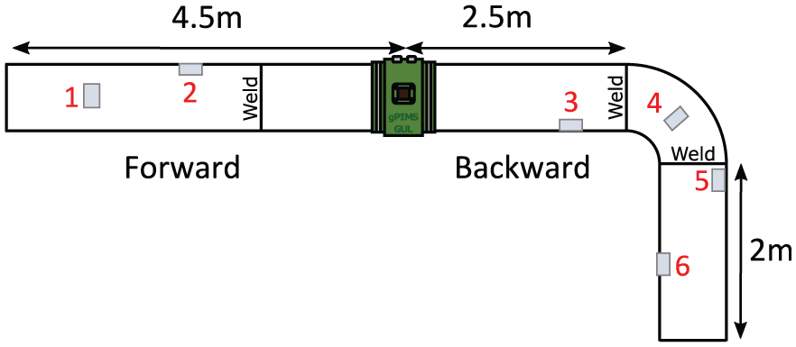
Setup of the pipe used to investigate performance of the SHM system. An 8-inch schedule 40 pipe of lengths 7 m and 2 m was connected by a 1.5D bend. Weld located at a distance of approximately 2 m in the forward direction. Defect positions highlighted in grey and numbered in red.

A heating cable was helically wrapped around the outside of the pipe, allowing for its temperature to be controlled. The setup was cycled between room temperature and 60°C while measurements were collected. About 300 baseline measurements were taken at various temperatures during cycling and prior to any introduction of damage. Defects were introduced into the pipe at six different locations as indicated in Figure 1. Three defects were placed on the long straight pipe section onto which the gPIMS was attached. A single defect was introduced on top of the 1.5D bend approximately half way along it, and two more damage sites were located past the bend. The defects were introduced into the setup by grinding away small amounts of material from the outside of the pipe using a diamond burr; no grinding was performed while a measurement was being made. The size of each of the defects was increased in 10 steps, after each of which precise measurements of its dimensions were taken; the cross-sectional area loss at each stage of the damage growth could thus be calculated. This article will focus on the growth of three out of the six defects – two on the longer of the two straight pipe sections (defects 1 and 2) and another close to a weld just past the pipe bend (defect 5). All three defects presented in this article were introduced at different times, that is, the defects were grown to their 10th and final stage before damage at a different location was initiated. Since the defects were relatively small, they have little effect on the signal transmitted past them and incident on any features further down the pipe; therefore, reflections from later defects will be little affected. However, a defect introduced between the monitoring ring and another defect will cause a change in the coherent noise floor past its location. This can affect the visibility of the later damage due to superposition of its reflection with the coherent noise.

FE models were created based on the measured dimensions of the defects during the growth process simulating the torsional T(0,1) guided wave reflections from these discontinuities. The predicted FE defect reflections could then be superimposed onto a number of damage-free collections of the test pipe section at the same locations at which the real defects were later introduced. Datasets with the real and the artificial defect reflections were then investigated using an ICA-based SHM algorithm so that the monitored growth for both cases could be compared. A flowchart of the procedure can be seen in Figure 2.

Figure 2.

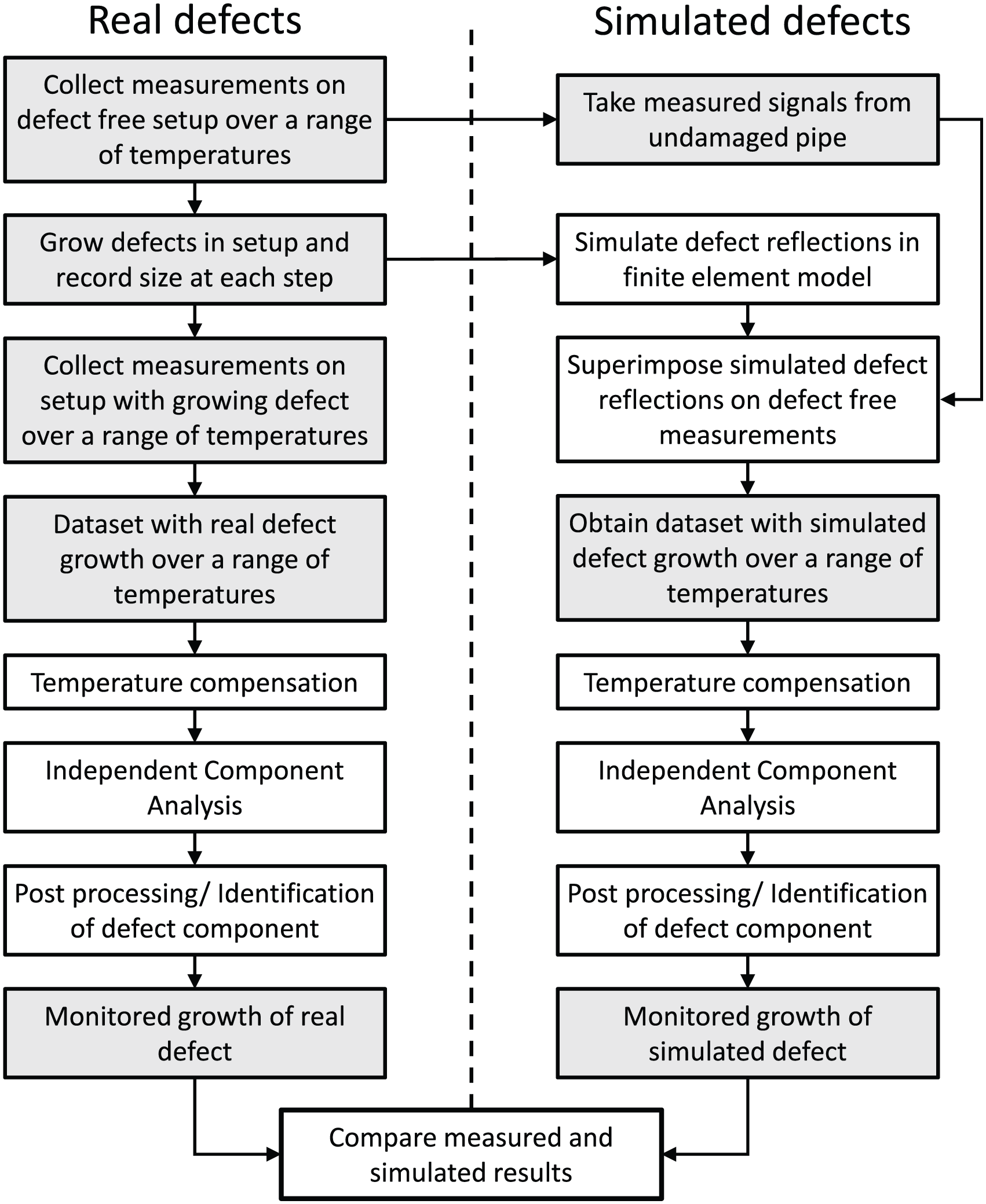
Schematic of process of comparing real defect growth to artificial defect growth superimposed onto real data collections. Grey boxes indicate data. White boxes indicate operations on data.

Data collection

For the proposed procedure of superimposing simulated defect reflections and real guided wave measurements, a large number of collections from the test pipe setup are required. A non-dispersive torsional T(0,1) guided wave signal was excited by the transducer ring which works in pulse-echo mode. The Hanning-windowed eight-cycle excitation signal used had a centre frequency of 25.5 kHz. An example plot of such a measurement, collected in both directions from the transducer ring location, can be seen in Figure 3. Due to the non-dispersive nature of the T(0,1) mode, all signals could be plotted in the spatial domain by simple conversion with the T(0,1) wave velocity in carbon steel. The signals are normalised to the cut end reflection of the straight pipe section (forward direction as determined by the sensor orientation). The reflection from the cut end past the pipe bend is significantly reduced in amplitude and the mode conversions induced by the passing of the signal through the 1.5D bend cause severe distortions in the shape of the reflected wave packet. The reflection from the weld at a distance of approximately 2 m from the transducer ring is highlighted in the plot. The pipe bend can be identified in the signal trace by the reflections from its two welds connecting it to the straight pipe sections, as seen in Figure 3 at approximately 2.5 and 3.2 m from the measurement position.

Figure 3.

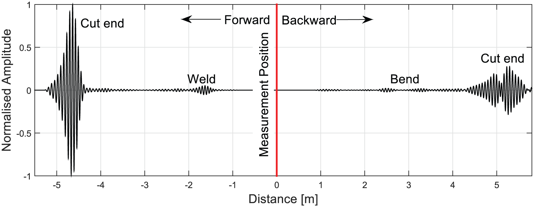
Example of A-scan measured on the defect-free test pipe in the forward and backward directions.

Artificial defects

With knowledge of the exact axial, circumferential and radial extent of the introduced defects, it was possible to replicate these using an FE model. This was achieved by first creating an undamaged mesh of the L-shaped pipe setup using ABAQUS CAE. The mesh was generated with 300 brick elements around the circumference of the pipe and 4 elements across the pipe wall thickness. The meshed geometry was exported to MATLAB in order to introduce defects of the same dimensions as those measured on the experimental setup over the course of the trial into the FE model. Using the measured dimensions of the real defects, ellipsoidal depressions were introduced into the pipe wall by compressing a number of elements of the FE mesh in the radial direction. Figure 4 shows a cut-away view of the mesh for defect 2 at its 10th and final growth stage. Individual FE models were generated for the 10 growth stages for each of the three investigated defects, yielding 30 models in total. The T(0,1) input signal was introduced into the FE model by displacing a ring of nodes on the surface of the pipe in the tangential direction. After introducing the desired defect shapes, the models were solved in the time domain using the ABAQUS explicit solver. This procedure has been reported in previous works.^5,6,17 A ring of monitor nodes was used to record displacements in all spatial dimensions. The T(0,1) mode was extracted by summing the tangential displacement of all the monitoring nodes, as discussed in Lowe et al. ¹⁸

Figure 4.

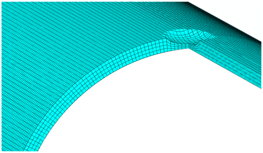
Cut-away view of FE mesh used to replicate the final growth stage of defect 2.

The changing temperature of the pipe was not considered when using FE simulations to generate defect reflections. This is reasonable as the reflection coefficient from a defect is unlikely to be significantly affected by the small temperature-induced material property changes. However, the position of the defect reflections when superimposed onto the baseline data was determined by the temperature of each guided wave collection, as the temperature-induced velocity changes do affect the arrival times. However, possible changes to the phase of the induced signals were not considered, which could cause some variation between results of real defects and those replicated via FE simulations.

Reflections from defects in the straight pipe sections positioned before the bend were simulated by analysing the reflections in a straight pipe; since the T(0,1) mode is non-dispersive, the propagation distances are not relevant as a time delay can be added as required during the superposition process. However, when considering reflections from defects located past the bend, it was important to include the approximate bend geometry in the model as the signal incident on the defect is significantly affected by propagation round the bend, and the time delay induced by the bend is not as simple to determine as for a length of straight pipe.

Rather than exciting the guided wave signal at the ring position, the T(0,1) mode was induced at the cut end of the pipe. This meant that the wave travelled only in one direction from the excitation, thereby avoiding early reflections from the free end that would complicate the signal. In the physical setup, this is dealt with by exciting on two adjacent rings and phasing the inputs to cancel the wave travelling in the unwanted direction; ¹⁹ this could have been implemented in the FE model but was an unnecessary complication. The phase delay between defect reflections recorded by the FE model and the test pipe section can easily be compensated for by shifting the signal in the time domain. Welds present in the trial pipe were neglected throughout the FE simulations as their influence on the defect reflections is minimal.

A torsional T(0,1) signal was introduced into the FE model by simultaneously displacing all the nodes in the excitation ring by the same amplitude in the circumferential direction, thus suppressing the generation of flexural wave modes. ² The Hanning input signal had a centre frequency of 25.5 kHz and a pulse length of eight cycles, identical to the input signal of the laboratory trial. Predicted reflections of the T(0,1) mode from the introduced defects were obtained by summing the circumferential displacements at a ring of monitoring nodes. ¹⁸ Using this setup, the reflections for each of the defects at each of their growth stages were recorded. An example plot of a number of reflected signals from defect 1 can be seen in Figure 5.

Figure 5.

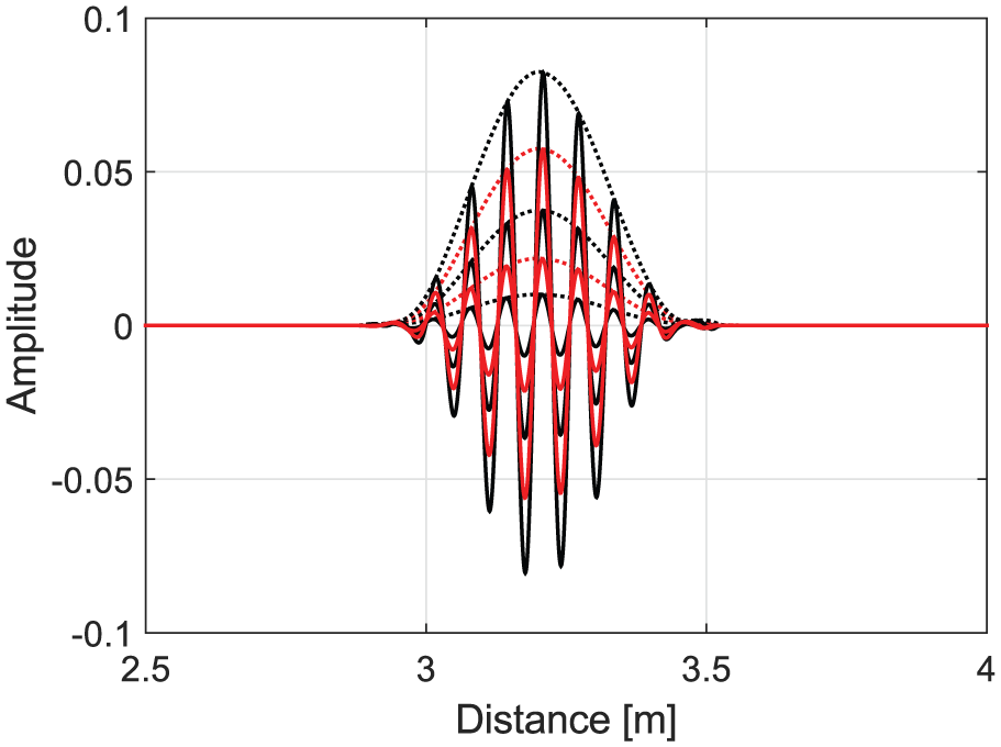
Example of reflections obtained from FE model of defects introduced into a straight pipe section. Five of the 10 stages of defect 1 are shown.

Combining real and artificial data

The next stage of the investigation consisted of combining the baseline data collected from the physical pipe setup with the reflection signals obtained from the FE simulations of the damaged pipe. Measured and simulated time traces were combined by simply superimposing the FE time traces onto baseline measurements. The exact location of the defect reflections was adjusted for the temperature of the baseline measurement, ensuring correct positioning relative to other pipe features and preventing misalignment after later temperature compensation of the signals. This was achieved by shifting the position of the simulated defect reflections in accordance with the temperature stretch factor of the respective baseline signal which was obtained as described in the following section. The baseline measurements were chosen such that a range of temperatures, comparable to the measurements collected during the real defect growth, was covered. The same number of undamaged pipe measurements was chosen for the growth of the artificial defect as was collected during the growth of the real damage on the laboratory pipe setup; also the number of measurements at each growth stage of the defect was kept consistent between the real and simulated defect datasets, so the performance of the SHM algorithm operating on both datasets could be compared directly.

Damage detection algorithm

For each of the three defects in the pipe setup investigated in this article, the SHM algorithm was applied to both the measurements of the real defect growth and the previously generated dataset containing the simulated defect growth superimposed onto defect-free measurements of the pipe. The first stage of the SHM algorithm consists of compensating each dataset for environmental variations by linearly stretching the signals to a baseline measurement by applying a scale transform–based temperature compensation algorithm. ²⁰ The optimal stretch factor is determined by maximising the correlation coefficient of the baseline and the signal to be compensated. An ICA algorithm is subsequently used to reveal underlying changes in each of the temperature-compensated datasets. ⁹ ICA allows a set of guided wave measurements to be decomposed into a number of weighting function and component pairs. Each of the obtained components corresponds to reflections from one or more features in the pipe. The corresponding weighting functions contain information about the change in the component reflection amplitude over the course of the dataset; this process has been described by Dobson and Cawley. ²¹ The mathematical background to ICA has been described by Hyvarinen and colleagues.^7,8,22 An example of this can be seen in Figure 6, where three-component and weighting function pairs are shown. These ICA results were obtained from a dataset of 20 normalised collections in the forward direction of the setup shown in Figure 1 over a range of temperatures. A synthetic defect was introduced at a distance of 3.5 m from the measurement location after the first 10 collections with a reflection amplitude of 3%. The defect growth can thus be seen in the first ICA output pair (Figure 6(a)). The component clearly shows a single feature reflection at 3.5 m and the weighting function indicates that the amplitude of this feature was at 0% for the first 10 collections of the dataset and then suddenly increased to 3%. Figure 6(b) corresponds to the ICA result related to the baseline signal of the measurements as indicated by the fact that the weighting function only varies slightly about 100% for the 20 measurements of the dataset and the component shows the reflection of the cut end of the test pipe at approximately 4.5 m. Figure 6(c) shows a component with random noise and a weighting function which varies at a very low amplitude. This can therefore be assumed to correspond to a noise component which would be of no interest to an investigator.

Figure 6.

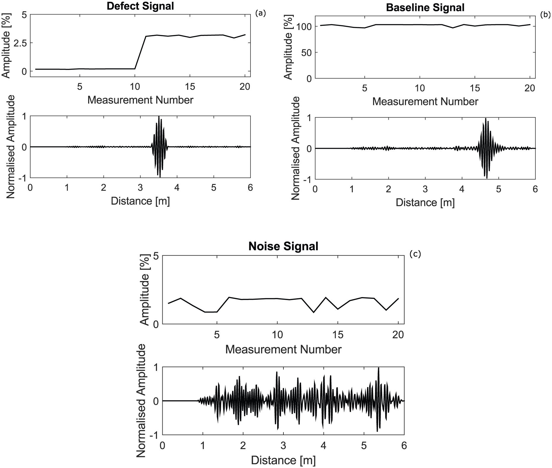
Component weighting function pairs after applying independent component analysis to an example set of 20 measurements: (a) Defect component shown with growth from 0% to 3% after 10 measurements, (b) baseline signal stable around 100% and (c) noise component with small variations at low amplitude.

Temperature is the only environmental variable considered in this study and the associated blind trial. ⁹ Variations in material temperature are a very significant factor making health monitoring applications more difficult to implement successfully.^23,24 There are, however, other issues such as contents or load, for example, which may be important in many instances.^25–28 The influence of a large number of environmental effects can manifest as variations in the coherent noise floor, thus reducing the damage detection ability of a system. If the baseline data collected contain these variations, they will be included in the data to which the stretch and ICA methodology of Figure 2 is applied. Provided these environmental changes do not affect the defect reflection amplitude and arrival time more than the temperature of the structure, the simulation approach will also work and so could be used to evaluate the system performance. However, this has not been tested here since the blind trial only included temperature variations.

The temperature of a pipe in the field will generally not be as uniform as for the pipe setup used in this investigation. Non-uniform temperature distributions across the length of an inspected structure might affect the results of any SHM approach used. Provided that the baseline data include these non-uniform temperature variations, the validation methodology will still work and it would be expected that the defect detection capability will be somewhat degraded. This cannot be verified using the trial data of Heinlein et al. ⁹ as the temperature was kept uniform over the full structure.

During the investigation presented in this article, the component and weighting function pairs corresponding to the growth of defects in the datasets were identified manually from the ICA results. The amplitude of the defect reflection over the course of the datasets obtained from the weighting functions, for both the simulated and real defect growth, could thus be compared to the actual cross-sectional area loss at each of the damage stages as measured during their introduction into the test pipe.

Results and discussion

The ICA-based SHM methodology was applied to the datasets with real and artificial defect growth after each of the 10 growth stages for defects 1, 2 and 5, positioned as seen in Figure 1. For each of the defects, two figures are plotted, the first of which shows the defect component at the time of first call, that is, when it was first detected during the blind trial. ⁹ The second plot presents the defect component and weight at its 10th and final growth stage. The weighting functions can be used to compare the defect growth patterns predicted from the real and synthetic datasets with each other and with the true defect growth.

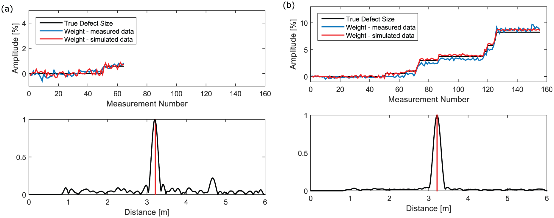
Figure 7 shows the results obtained for defect 1, located on the longer straight section of the test pipe in the forward direction. The components shown in Figure 7(a) and (b) for the first detection and final stages show that in both cases the defect was correctly located at a distance of 3.46 m from the transducer ring, which is shown by a vertical red line on the plots. In Figure 7(a) it can be seen that the defect growth pattern identified was similar for the real and simulated defect datasets, the growth at around measurement 50, being evident in both. The damage in this case was identified after it had been grown to its fourth stage corresponding to a cross-sectional area loss of 0.63%. The weighting functions obtained from both the simulated and measured data follow the true CSA level as determined from the defect dimensions. Deviations from the true defect size as well as variations in the defect amplitude during periods when its size was not changing can be attributed to the varying temperatures of the pipe and imperfectly compensated environmental effects. An example of this can be seen in the weighting function in Figure 7(a) around measurement number 100. Here, the baseline data onto which the simulated defect reflection was superimposed underwent a full temperature cycle. Figure 7(b) shows that both the simulated and real defect components follow the true defect size closely. For the two final growth stages, the weighting function obtained from the measured data underestimates the size of the defect slightly; this was because defect 2 was then also being introduced into the pipe, causing changes in the coherent noise at the location of defect 1 which destructively interferes with the defect reflection. This effect was not modelled in the simulations.

Figure 7.

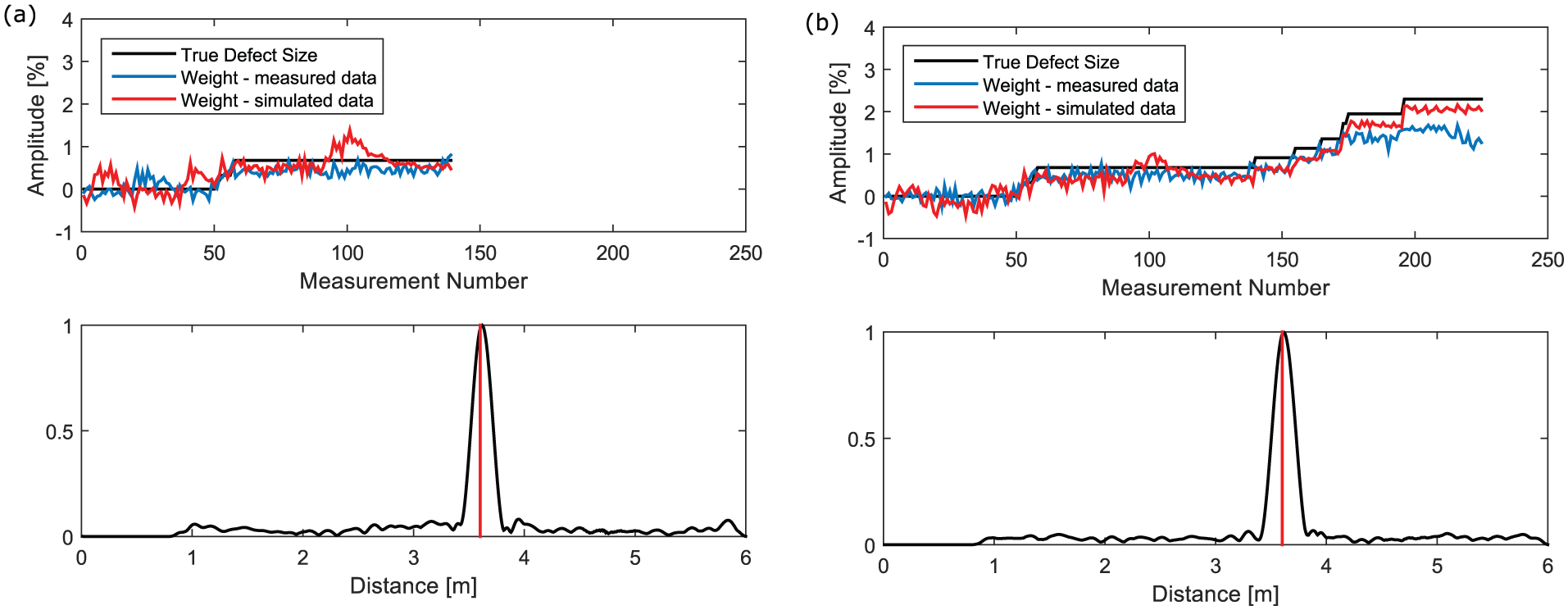
Weighting functions for defect 1 (a) at time of first detection after 4 growth stages and (b) at its final size after 10 growth stages. The weighting function in black indicates the true damage size, blue shows the ICA weighting function using measured data and red shows the ICA weighting function using simulated data. The plotted components in (a) and (b) are those obtained from the real defect growth dataset. The position of the defect as measured on the pipe during the trial is indicated by a vertical red line.

The ICA results of defect 2, located on the straight section of the pipe in the forward direction, are shown in Figure 8. The components at both the time of first detection and the final growth stage indicate that the defect was identified at the correct distance of 2.57 m from the transducer ring. The defect was first detected after five growth stages with a cross-sectional area loss of approximately 0.73% in the datasets of the real and simulated growth. The growth of the measured and simulated weighting functions is first evident around measurement number 90. In both cases, the weighting functions trace the true defect size well. Similar to the results for defect 1, the discrepancies between the expected and observed amplitude of the weighting functions can be attributed to imperfectly compensated temperature effects. Figure 8(b) shows the results of the SHM procedure after the defect had grown to its final size with a cross-sectional area loss of 1.8%. It can be seen that the weighting functions of both the simulated and measured data trace the true defect size well.

Figure 8.

Weighting functions for defect 2 (a) at time of first detection after 5 growth stages and (b) at its final size after 10 growth stages. The weighting function in black indicates the true damage size, blue shows the ICA weighting function using measured data and red shows the ICA weighting function using simulated data. The plotted components in (a) and (b) are those obtained from the real defect growth dataset. The position of the defect as measured on the pipe during the trial is indicated by a vertical red line.

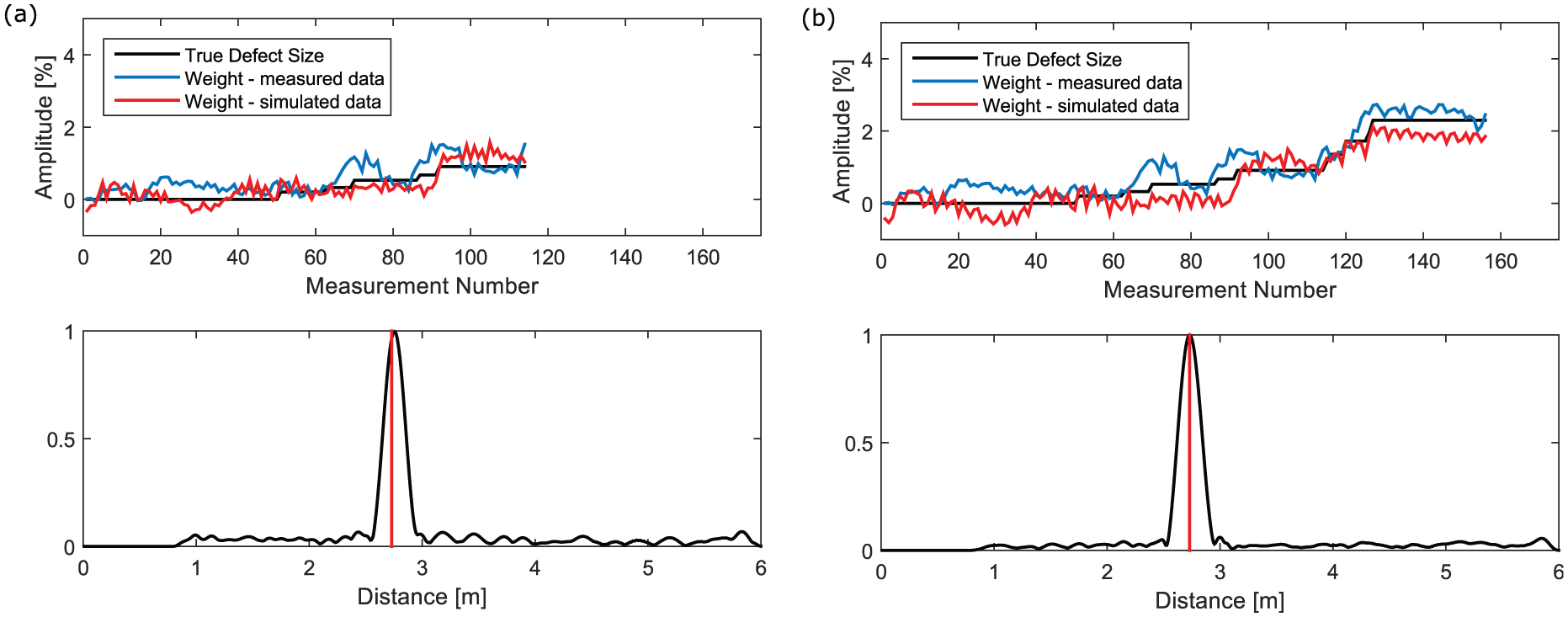
The results of the last defect investigated in this article are shown in Figure 9(a) and (b). Defect 5 was introduced into the test pipe close to a weld just after the 1.5D pipe bend. During the trial, it was initially expected that defects positioned past the pipe bend would be more challenging to identify and thus defect 5 was grown in larger increments and to a greater final size in comparison with the defects introduced before the bend. The defect was first detected during the trial after completing its first growth stage, resulting in a cross-sectional area loss of 0.59%. Figure 9(a) shows the results of the ICA-based SHM procedure at the time of first detection. A clear step in the weighting functions is visible around measurement number 50. Consistent with the results for defects 1 and 2, the weighting functions of both the simulated and the measured data trace the true defect size closely. Over the full 10 growth stages of the defect, the weighting functions of both the simulated and measured datasets track the defect size well, as seen in Figure 9(b); it should be noted here that the weighting functions in Figure 9(a) and (b) are plotted on different amplitude scales. Variations in the amplitude of the weight in Figure 9(b) with respect to temperature are not as prevalent as for the two previously presented defects; this can be attributed to the larger final size (8.27% CSA) of defect 5 diminishing the effect of temperature variations.

Figure 9.

Weighting functions for defect 5 (a) at time of first detection after the first growth stages and (b) at its final size after 10 growth stages. The weighting function in black indicates the true damage size, blue shows the ICA weighting function using measured data and red shows the ICA weighting function using simulated data. The plotted components in (a) and (b) are those obtained from the real defect growth dataset. The position of the defect as measured on the pipe during the trial is indicated by a vertical red line.

Conclusion

Validating the performance of guided wave SHM systems is vital if they are to be widely deployed; testing the damage detection ability of a system by introducing different types of damage at varying locations is very costly and cannot be performed on a system in operation. A performance validation methodology making use of large numbers of defect-free measurements of a system and superimposing defect reflections obtained from FE simulations has previously been proposed and shown to be successful on a rudimentary laboratory pipe setup.

A blind trial was recently conducted in order to test the performance of guided wave SHM systems for pipes. A number of defects were introduced into a pipe setup including welds and a 90° bend. The setup underwent temperature cycling while measurements were collected and the locations, growth rates and dimensions of the defects were recorded. The measurements therefore provided an opportunity to investigate the accuracy of the proposed performance validation methodology on a representative pipe system.

The growth of three of the defects in the test pipe was replicated by superimposing synthetic defects, obtained from FE simulations of the damage, onto readings acquired during environmental cycling of the pipe prior to the introduction of any damage. This allowed for the generation of datasets with well-defined defect growth patterns at known locations while also retaining the effects of environmental variations of the structure on the signals which cannot be obtained from FE simulations. The datasets containing the simulated defect growth were processed with the same ICA-based SHM procedure as used for the initial defect identification during the blind trial. The ICA procedure yields the estimated defect location and its growth as a function of time. Very good agreement was obtained between the results obtained using the purely experimental data collected during the blind trial and those obtained from the synthetic datasets, both corresponding well with the true defect growth. The results obtained during the investigation therefore validate the proposed performance prediction methodology.

The ability to validate the damage detection ability of an installed health monitoring system will be of significant value in the development of safety cases as it will be possible to establish whether a defect of a particular size, location and type would be detected by the setup. By combining measurements collected during environmental cycling of the system and simulated defect reflections obtained from FE studies, the minimum defect size detectable with the SHM system for a test structure can be determined. The presented methodology enables the operator to combine the ability of FE analysis to predict the signals reflected from a large number of different defect cases with the complex geometric and environmental effects specific to the particular pipe structure which cannot be effectively simulated. Although the results presented in this article were obtained from a guided wave system for pipes, this methodology can be utilised to predict the damage detection ability of any other SHM system.