
Abstract
Reconstruction of structural health monitoring data is a challenging task, since it involves time series data forecasting especially in the case with a large block of missing data. In this study, we propose a novel methodology for structural health monitoring data recovery in the context of Bayesian multi-task learning with multi-dimensional Gaussian process prior. The proposed methodology stands to model a series of tasks simultaneously rather than modeling each task independently while explicitly encoding the correlations among tasks that can be learnt efficiently from data. The primary advantage of Bayesian multi-task learning for data reconstruction is that it makes more efficient use of the data available and gives rise to enhanced reconstruction capability by making use of the underlying task relatedness. Since the modeling performance of the Gaussian process–based Bayesian approach heavily relies on the selected covariance function, particular focus has been laid on the influences of various kinds of covariance functions including the unblended and composite (hybrid) ones on reconstruction performance. The instrumented Canton Tower of 600 m high is used as a test bed to illustrate the effectiveness of the proposed method in reconstruction of structural health monitoring data. The traditional Bayesian single-task learning approach is also implemented for comparison purpose. The reconstruction results of the structural health monitoring data show that the proposed Bayesian multi-task learning methodology affords an excellent performance, while the Bayesian single-task learning method is unreliable in certain cases; yet, the selection of covariance function has a significant impact on the reconstruction performance of the proposed methodology. The work presented in this study also gains insight into how to choose an appropriate covariance function for reconstruction of missing structural health monitoring data.
Keywords
Introduction
Maintaining the efficient, reliable, and safe operation of vital infrastructure systems such as long-span bridges, dams, and high-speed railways is critical to securing the well-being of people, protecting significant capital investments and sustaining the vitality of regional and national economy. Structural health monitoring (SHM), on a continuous basis, provides plentiful information regarding structural behavior by various sensors and traces the health status of existing structures in real time so that early warnings could be signaled before catastrophic failure happens.1–5 Integration of SHM into lifecycle management strategy allows structural operators and asset managers to rate the structural performance in a real-time way and conduct maintenance and remedial actions in accordance with the in-service condition of an infrastructure system throughout its life cycle. Generally, SHM is the process of conducting condition diagnosis and prognosis for structural components or an entire system based on appropriate analyses of in situ monitoring data successively accumulated by an array of sensors deployed on the structure. 6 As a consequence, the accuracy and reliability of the structural condition assessment results directly depend on the quality and quantity of the monitoring data. However, data missing is a common occurrence during the long-term monitoring process owing to sensor faults or failures that can be caused by a variety of reasons, including power depletion, hardware failure, a lack of timely maintenance, harsh environmental attack, to name but a few. It is highly desirable to reconstruct the missing data for the subsequent analysis in order to achieve an accurate evaluation of structural health condition.
The research topic of missing data reconstruction has been widely explored in a variety of fields, such as geophysics, 7 biology, 8 and image processing. 9 In the field of SHM, the reconstruction of missing SHM data has attracted increasing attention from researchers and numerous methods have been proposed, such as transmissibility concept,10,11 inverse optimization scheme,12,13 empirical mode decomposition (EMD) combined with finite element (FE) modeling.14,15 However, these approaches, which belong to the model-based family, require an FE model of the structure to recover the incomplete measurement data. The nature of the model-based approaches limits their applicability in the recovery of site-specific monitoring data (structural responses, and loading and environmental effects) for complex, large-scale infrastructure systems under changing environmental and operational conditions, since it is extremely difficult or even impossible to formulate an accurate FE model that is representative of the authentic behavior of the in-service structure. As an alternative to the model-based approach, the data-driven approach does not rely on an FE model and performs analyses directly on the measured time series data, making it potentially powerful in solving SHM problems for large-scale structures. The data-driven approach is intended to formulate a statistical model of time series aiming to extract damage-sensitive features or reveal the underlying patterns that can be utilized to characterize structural health state.
In the SHM literature, a variety of time series modeling techniques have been proposed, including state-space (SS) model,16,17 autoregressive (AR) model,18–23 Gaussian process (GP) model,24–26 among others. These time series models have been extensively investigated for a wide range of SHM applications such as structural condition classification, sensor fault diagnosis, and signal outlier detection, but they had seldom seen applications in the reconstruction of incomplete SHM data. Missing data reconstruction is in essence the solution of a forecast problem; more specifically, a time series model will be formulated using the available measurements to estimate the missing values. Satisfactory reconstruction of very few missing data during a short time interval or a relatively large amount of missing data uniformly spaced over the whole time scale can be readily achieved, since most modeling tools perform well for a wide range of interpolation scenarios but only for a small range of extrapolation scenarios (e.g. limited-step ahead forecasting). Although among a variety of time series models, the probabilistic, nonparametric GP model which is built in the context of Bayesian inference manifests high modeling flexibility and great expressive power, its extrapolation prediction capability is fairly limited. As reported by Wan and Ni, 26 the forecasting error associated with GP model becomes larger as the step of the ahead forecasting increases. In an attempt to enhance the forecasting accuracy of GP model for missing data reconstruction, we propose the use of the multi-task learning (MTL) strategy in this study to improve the out-of-sample forecast performance by taking advantage of the task similarity.
MTL has gained a surge of research interest in the data mining and machine learning community with the purpose of classification, regression, and clustering. 27 In the MTL paradigm, a collection of related tasks are learned jointly by extracting appropriate shared information across the tasks. It is expected that the intrinsic relationships among these tasks can be fully exploited and learning them simultaneously can lead to better generalization performance than learning each single task separately; the latter is referred to as single-task learning (STL). The advantage of MTL over STL tends to be more pronounced in the circumstances when training samples are insufficient to uncover the latent models, and when a set of samples over specific range are missing for certain tasks, but yet available for other related tasks. MTL has been recognized to be a powerful learning tool for a wide range of practical applications including speech recognition, disease progression prediction, document categorization, and so on. From a Bayesian perspective, MTL can be implemented naturally by placing a common prior distribution over either of the shared parameters that define the different models or the multivariate outputs. Bonilla et al. 28 proposed a Bayesian MTL framework with multivariate GP prior over multiple tasks. More specifically, a separable covariance structure expressed as a Kronecker product of the input covariance function and the task covariance matrix is used for the specification of GP distribution of a collection of tasks. The GP-based Bayesian MTL has been successfully used in many areas including robot dynamics, neuroimaging, and clinical analysis. It is also worth mentioning that Bayesian-based approaches have been widely adopted in SHM for both model-based implementation29–34 and data-driven solution.35–39
In recognition of its strong capability in modeling time series data collectively, GP-based Bayesian MTL is proposed in this study for reconstructing incomplete SHM data. In particular, the influence of different types of covariance functions, including the standard ones and the composite ones resulting from addition and multiplication operations, on reconstruction performance of the proposed Bayesian MTL methodology is investigated in detail, aiming to provide useful guidance on selection of an appropriate covariance function for reconstructing incomplete data. Although the Bayesian MTL methodology developed in this work is concerned with the reconstruction of missing SHM data, it is worth mentioning that the proposed method is also applicable to the problems of sensor fault diagnosis, change-point detection, and structural condition classification. The rest of the article is organized as follows. In section “Bayesian modeling with GP prior,” the Bayesian MTL-based data reconstruction methodology is presented thoroughly, together with the formulation of the traditional STL model with GP prior. Section “Canton Tower and on-structure monitoring system” describes a supertall building and its on-structure long-term SHM system, which serves as a test bed for verification study. In section “Reconstruction of SHM data from Canton Tower,” the real-time temperature and acceleration monitoring data from the instrumented structure are utilized to demonstrate the reconstruction capability of the proposed Bayesian MTL methodology with different settings of covariance functions. We finally conclude in section “Conclusion” with a summary of this work.
Bayesian modeling with GP prior
Single-task GP model
We first give a brief introduction to the traditional GPM which deals with univariate output, termed as single-task GPM (STGPM). GP is a stochastic process where any finite subset of a collection of random variables has a joint Gaussian distribution.
40
The GP prior over latent function evaluations is fully specified by its mean function and covariance function. The mean function is in general set to be zero without loss of generality. Setting zero mean function is mainly because the prior brief about the latent function’s overall trend is usually unavailable.
41
In contrast, a variety of covariance functions exist in the literature, such as well-known squared exponential (SE) function, Martern (MA) function, and periodic (PE) function. If

with


In many realistic scenarios, we only have the observations that will be used to infer the latent function. The observation model that maps the relationship between the observations and the function values can be expressed as follows

where the independent and identically distributed (i.i.d.) Gaussian noise
Given a training data set
where


By applying Bayes’ theorem, the posterior distribution of
with the mean and variance given by

where
Multi-task GP model
In contrast with the STGPM that models each task independently, the multi-task GPM (MTGPM), as shown in Figure 1, is configured to learn all tasks simultaneously by taking into account the correlation among them. However, the implementation of MTGPM proceeds in a manner analogous to STGPM; the former can be realized through extending the latter by presuming the latent function
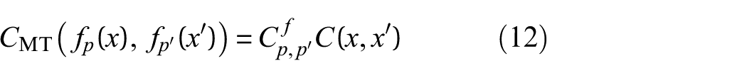
where the input covariance function
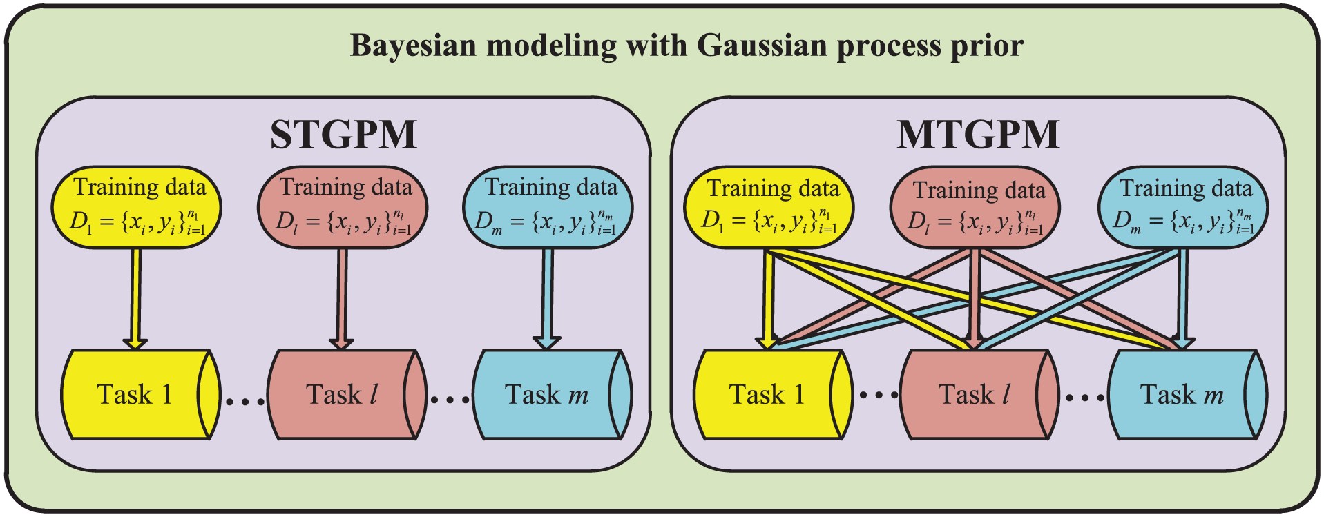
Modeling paradigms of STGPM and MTGPM.
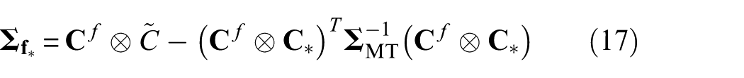
The above separable multi-task kernel with a free-form task covariance matrix

where
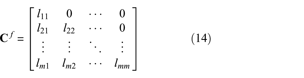
where m is the number of tasks. Aside from guaranteeing the positive definiteness of task covariance matrix, the use of the Cholesky decomposition also enables modelers to significantly reduce the number of the parameters to define
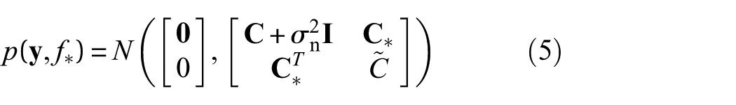
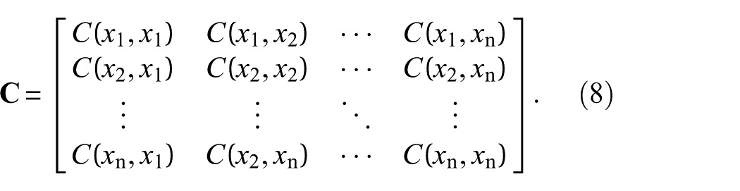
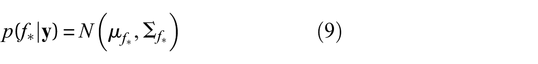
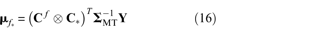
MTGPM is concerned with mapping the multivariate simulator

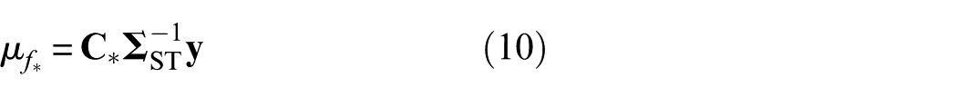
with the mean and variance given by
where
Covariance function
Since zero mean function is presumed for both STGPM and MTGPM and the free-form task covariance matrix is predetermined for MTGPM, the remaining task is the definition of an appropriate covariance (kernel) function, which may have a crucial impact on the modeling flexibility and expressive power of the GPM. The selected covariance function will encode our prior distribution over the underlying function which we wish to learn. The only constraint on a valid covariance function is that its created covariance matrix must be definite positive. However, it is not easy to choose a reasonable covariance function in practical applications. A wide variety of covariance functions are available within the GP framework; 40 among them three popular families of covariance functions are considered in this study. The first two are the SE covariance function and MA covariance function, which are commonly used in engineering and statistical communities, and the third one is PE covariance function which, as its name suggests, is effective for modeling a physical system whose outputs exhibit a PE or cyclic pattern.
The SE covariance function has the form
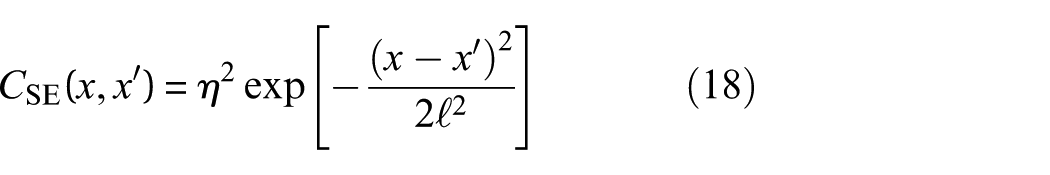
where
In this regard, for certain practical applications, the SE covariance function might be too restrictive. We, then, resort to the MA covariance function in the form of
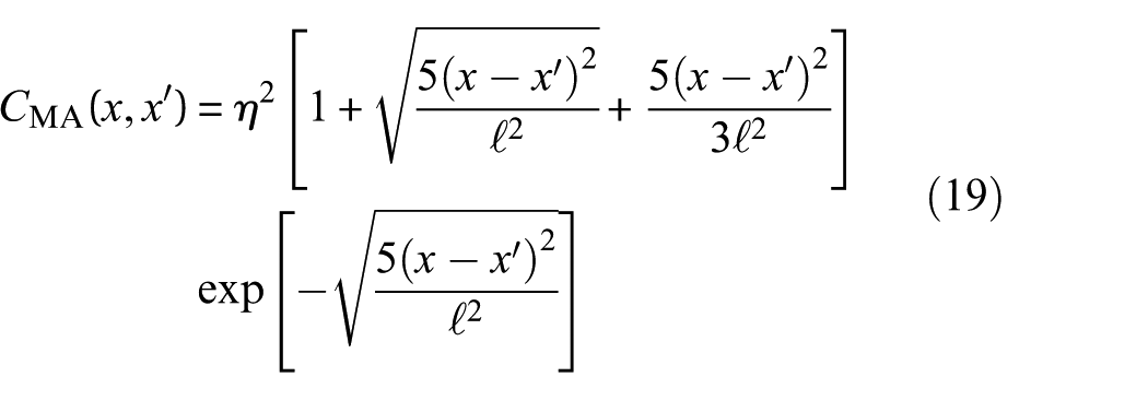
The MA covariance function results in the fitted function being twice differentiable, but not infinitely differentiable, so the MA covariance function is more appropriate for modeling significantly rough variations compared to the SE covariance function.
The final covariance function under consideration is the PE covariance function, expressed as follows
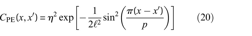
where p is the period characteristic. The PE covariance function is suitable for functions with PE behaviors; it would be helpful to model SHM data that exhibit seasonal variations.
Product or sum of two different types of covariance functions provides an effective way to generate composite (hybrid) covariance functions. Given that SHM data contain seasonal component, the hybrid covariance functions, which are the combination of either SE or MA covariance function with the PE one by using sum and product operations, respectively, are considered in this study. In summary, a total of seven covariance functions are explored, that is, SE, MA, PE, “SE × PE,”“MA × PE,”“SE + PE,” and “MA + PE.”
Estimation of hyperparameters
Now we turn to the estimation of hyperparameters that govern the GPMs. The hyperparameters in a GPM include the covariance function parameters and noise parameter. As for the MTGPM, covariance function parameters are composed of two parameter groups: one related to the input covariance function and the other related to the task covariance matrix. For instance, when the SE covariance function is selected to define both STGPM and MTGPM, the resulting hyperparameters are
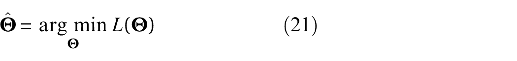
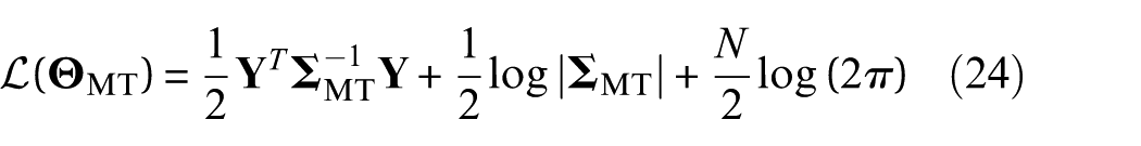
The objective function
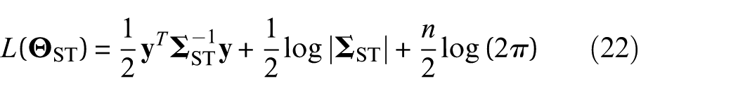
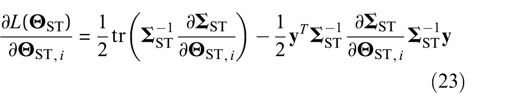
where |•|,
where
Since the log-likelihood function may be non-convex, the optimization solution is likely to suffer from multiple local optima. To reduce the risk of getting trapped in local minima, the multi-starting point strategy is utilized here in conjunction with the conjugate gradient (CG) optimizer for hyperparameter estimation.44,45 Specifically, a total of 100 starting points are randomly generated. Then the NLML value is computed for each case, and among them, 10 starting points corresponding to the smallest NLML values are selected as starting values to run the CG routine. Finally, the resulting hyperparameters with the smallest NLML value among these 10 pre-selected cases are accepted as the optimal set of hyperparameters.
Canton Tower and on-structure monitoring system
Description of Canton Tower
The Canton Tower, formerly known as Guangzhou New TV Tower, located in Guangzhou, China, assures a place among the supertall structures worldwide owing to the virtue of a total height of 600 m. This high-rise building comprises two structural portions: a 454-m-high main tower and a 146-m-high antennary mast. The main tower is a tube-in-tube structure consisting of a steel lattice outer structure and a reinforced concrete inner structure. The outer structure has a hyperboloid form, which is generated by the rotation of two ellipses, one at foundation level of the main tower and the other at an imaginary horizontal plan 454 m above the ground. The tightening resulting from the rotation between the two ellipses forms a “waist” halfway up the tower. These two ellipses are rotated relative to one another, yielding the dynamic turning tower with a “waist” halfway up.
The main tower of tube-in-tube structural form consists of a reinforced concrete inner tube and a steel outer frame tube. The outer tube is composed of 24 concrete-filled-tube columns, which are uniformly spaced in an ellipse shape with varying size ranging from the maximum of 50 m × 80 m at the base to the minimum of 20.65 m × 27.50 m at the waist level and are interconnected transversely through steel ring beams and bracings. In contrast, the shape of the inner tube is a constant ellipse with the cross-section of 14 m × 17 m. The inner and outer tubes are linked via four levels of connecting girders and 37 functional floors, providing a variety of services such as utilities, tour, catering, and TV and radio signal transmission facilities. On the top of the main tower is the antennary mast, which is a steel spatial structure with an octagonal cross-section of 14 m in the maximum diagonal.
SHM system
To ensure the safety of the Canton Tower in both in-construction and post-construction (in-service) stages, a sophisticated long-term SHM system has been implemented for integrated in-construction and in-service monitoring of this landmark building.47,48 After completing the erection of the structure in May 2009, the permanently deployed SHM system operates with a total of over 800 sensors of various kinds, such as GPS system, accelerometers, wind pressure meters, FBG temperature and strain sensors, and digital video cameras. The temperature and acceleration monitoring data acquired will be used in this study to demonstrate the applicability of the proposed Bayesian MTL-based data reconstruction methodology. Figure 2 shows the deployment of both temperature sensors and accelerometers on the Canton Tower, and the location details of the used temperature sensors are illustrated in Figure 3.
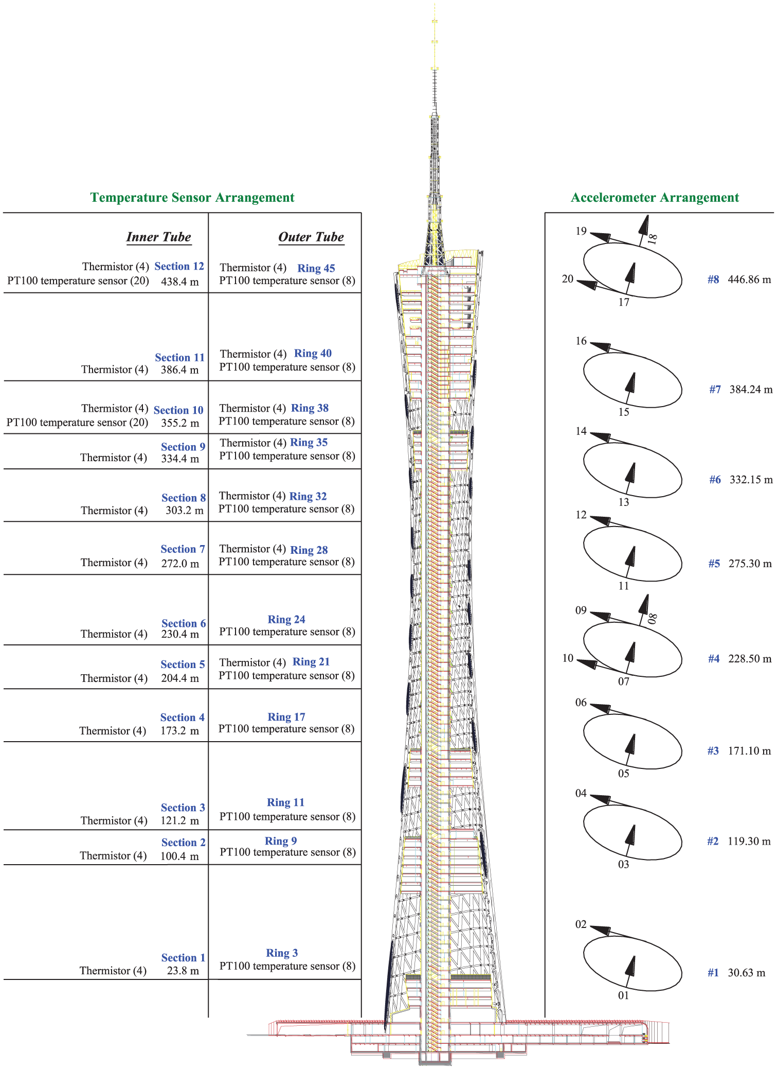
Deployment of temperature sensors and accelerometers on Canton Tower.
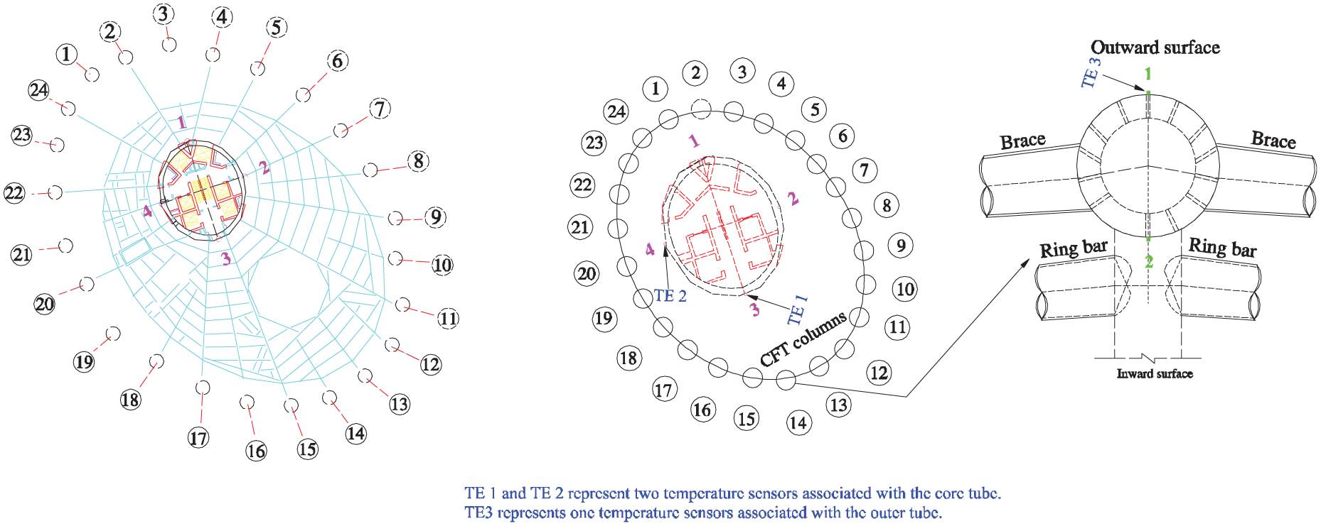
Location details of the temperature sensors concerned.
Reconstruction of SHM data from Canton Tower
Reconstruction of temperature measurements
The temperature data are used first to demonstrate the reconstruction capability of the proposed Bayesian MTL methodology. Without loss of generality, three temperature sensors deployed at cross-section 5, as shown in Figure 3, are selected to demonstrate the reconstruction capability of the proposed Bayesian MTL methodology. Specifically, two of them are associated with measurement points 3 and 4 of inner tube, while the remaining one is associated with measurement point 1 of outer tube, as shown in Figure 3. For illustration convenience, these three temperature sensors are denoted as “TE 1,”“TE 2,” and “TE 3,” respectively. Figure 4 shows the daily maximum temperature data in the year of 2014 monitored by the three temperature sensors in concern.
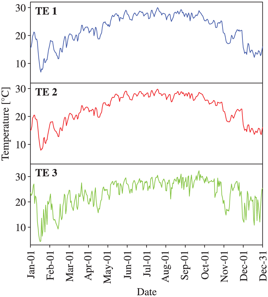
Monitored daily maximum temperatures in 2014.
In this study, one-sixth of the total monitoring data from one temperature sensor is removed to simulate missing data. To fully explore the influence of location(s) of missing data and different combination of tasks on data reconstruction capability of MTGPM, a total of five cases are introduced as follows:
Case 1. Missing data location is at the end of task “TE 1,” and tasks “TE 1” and “TE 2” are used for MTGPM formulation.
Case 2. Missing data location is at the end of task “TE 1,” and tasks “TE 1” and “TE 3” are used for MTGPM formulation.
Case 3. Missing data location is at the end of task “TE 1,” and tasks “TE 1,”“TE 2,” and “TE 3” are used for MTGPM formulation.
Case 4. Missing data locations are at the end of task “TE 1” and at the beginning of task “TE 2,” and tasks “TE 1” and “TE 2” are used for MTGPM formulation;
Case 5. Missing data locations are at the end of both tasks “TE 1” and “TE 2,” and tasks “TE 1” and “TE 2” are used for MTGPM formulation.
The first three cases consider missing data at only one task while having different pools of training data, aiming to investigate the effect of different task groups, whereas the rest two cases consider missing data at two tasks simultaneously and at different slots, seeking to examine the effect of missing data at multiple tasks and different slots. Meanwhile, STGPM is also formulated to reconstruct missing data for comparison purpose. Notice that STGPM just needs to consider a total of three cases since the first three cases above with the same single task suffering from data missing reduce in essence to an identical case for STGPM. Figures 5 to 9 illustrate the reconstructed temperature data by MTGPM for the five cases, and Figures 10 to 12 display the reconstruction results obtained by STGPM.
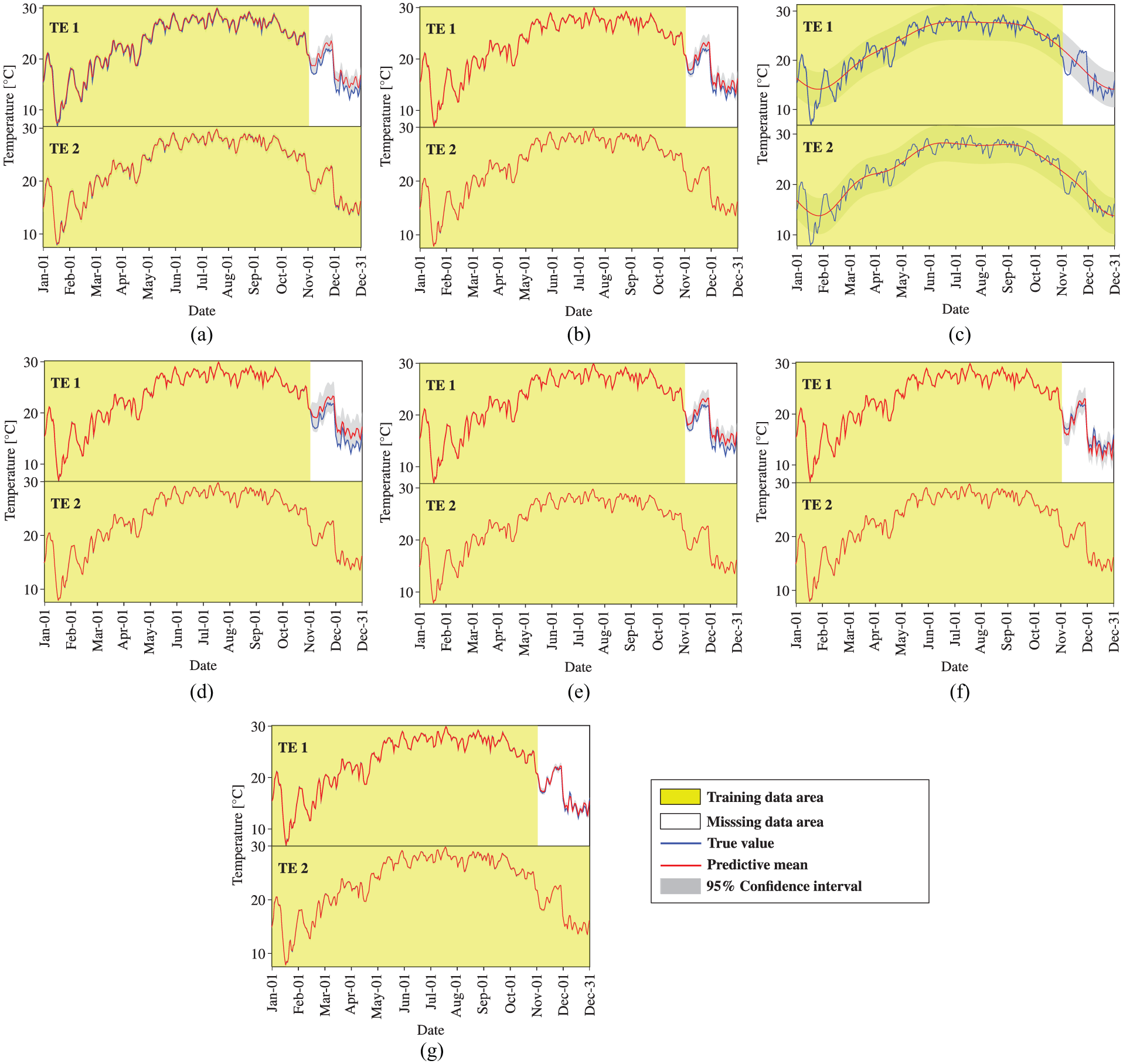
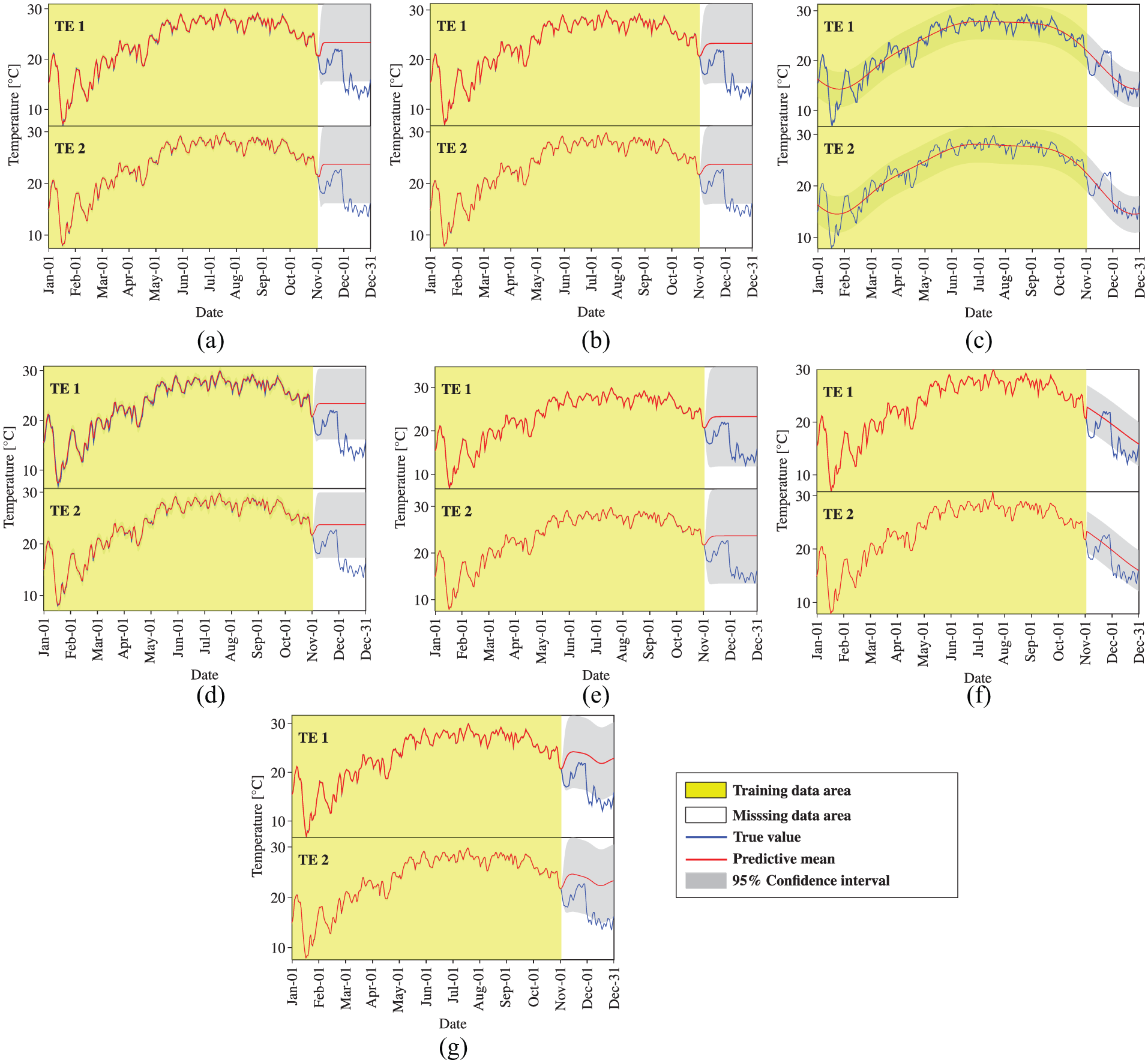
Temperature data reconstruction by MTGPM with different covariance functions (Case 1): (a) SE, (b) MA, (c) PE, (d) SE × PE, (e) MA × PE, (f) SE + PE, and (g) MA + PE.
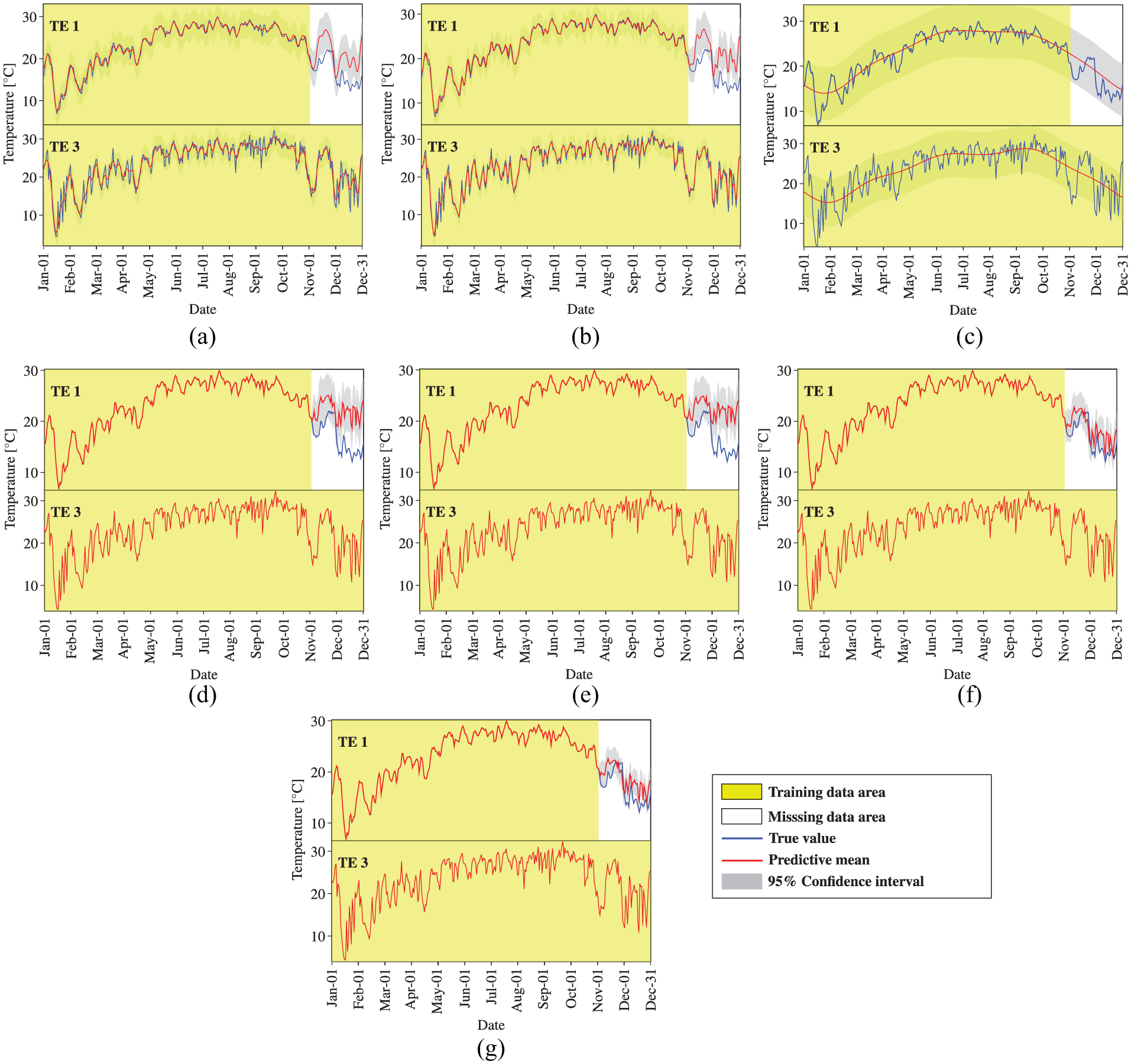
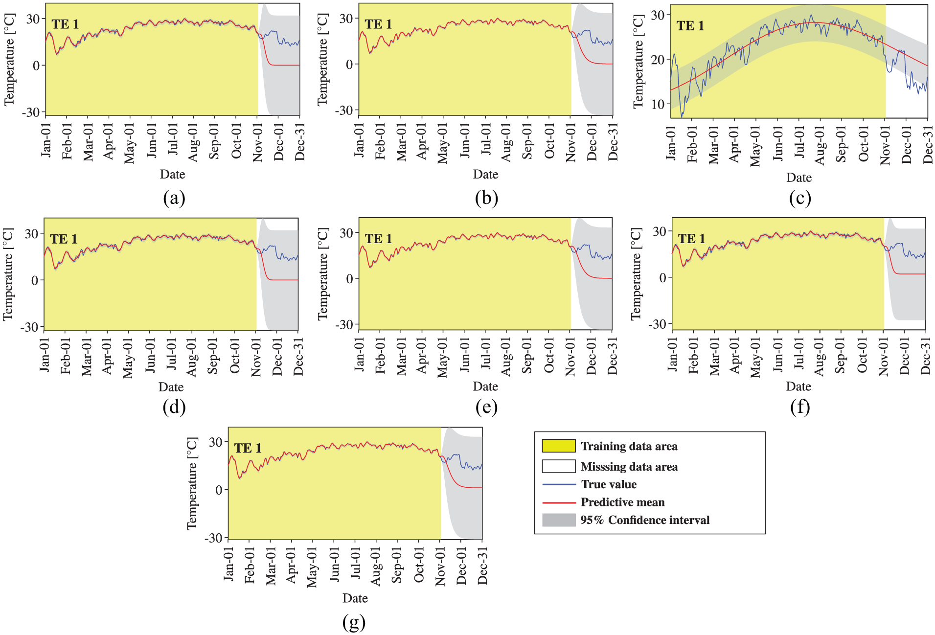
Temperature data reconstruction by MTGPM with different covariance functions (Case 2): (a) SE, (b) MA, (c) PE, (d) SE × PE, (e) MA × PE, (f) SE + PE, and (g) MA + PE.
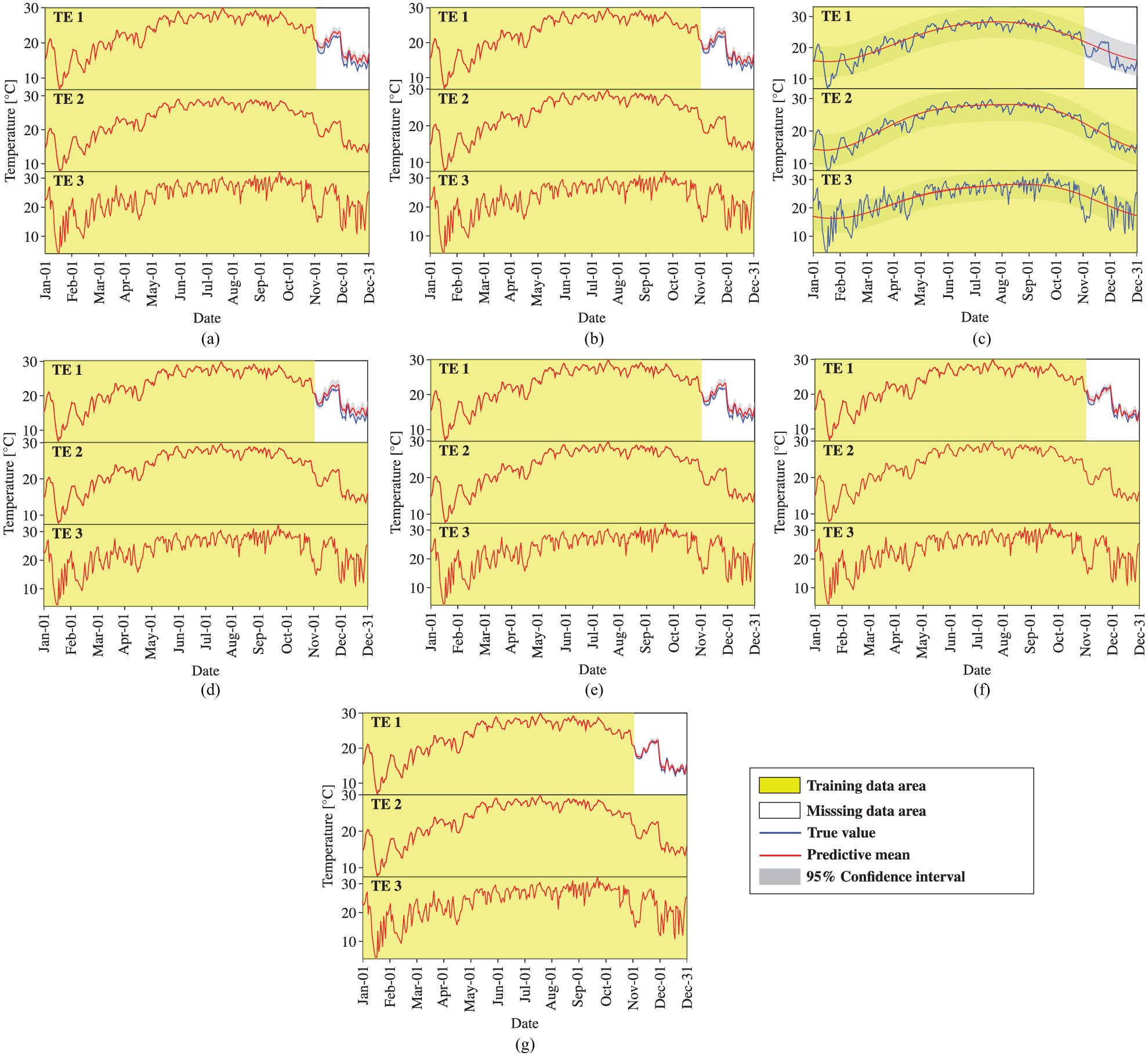
Temperature data reconstruction by MTGPM with different covariance functions (Case 3): (a) SE, (b) MA, (c) PE, (d) SE × PE, (e) MA × PE, (f) SE + PE, and (g) MA + PE.
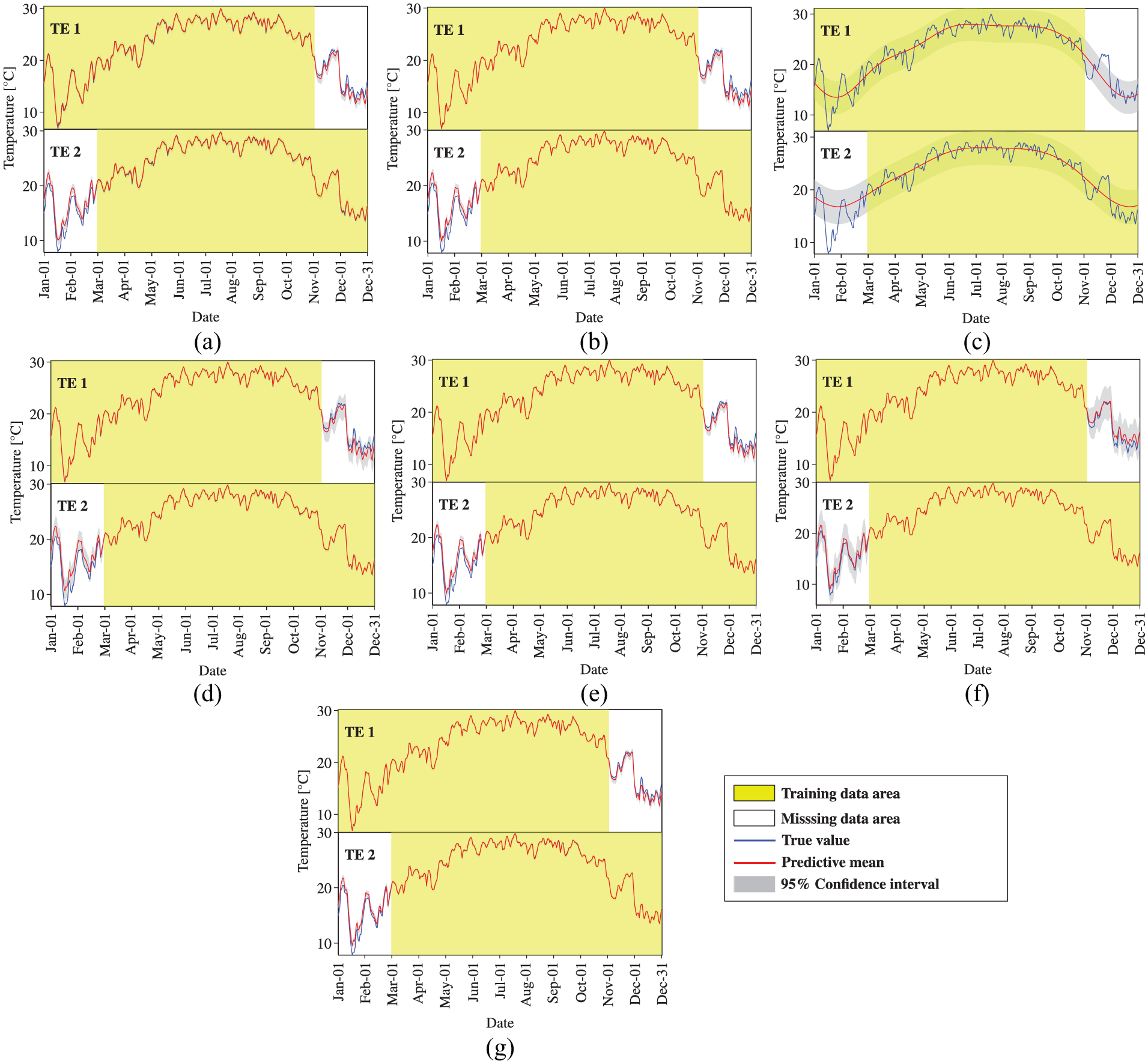
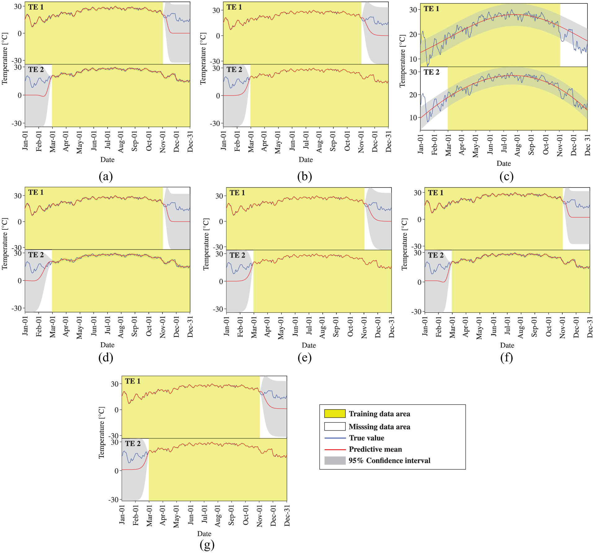
Temperature data reconstruction by MTGPM with different covariance functions (Case 4): (a) SE, (b) MA, (c) PE, (d) SE × PE, (e) MA × PE, (f) SE + PE, and (g) MA + PE.
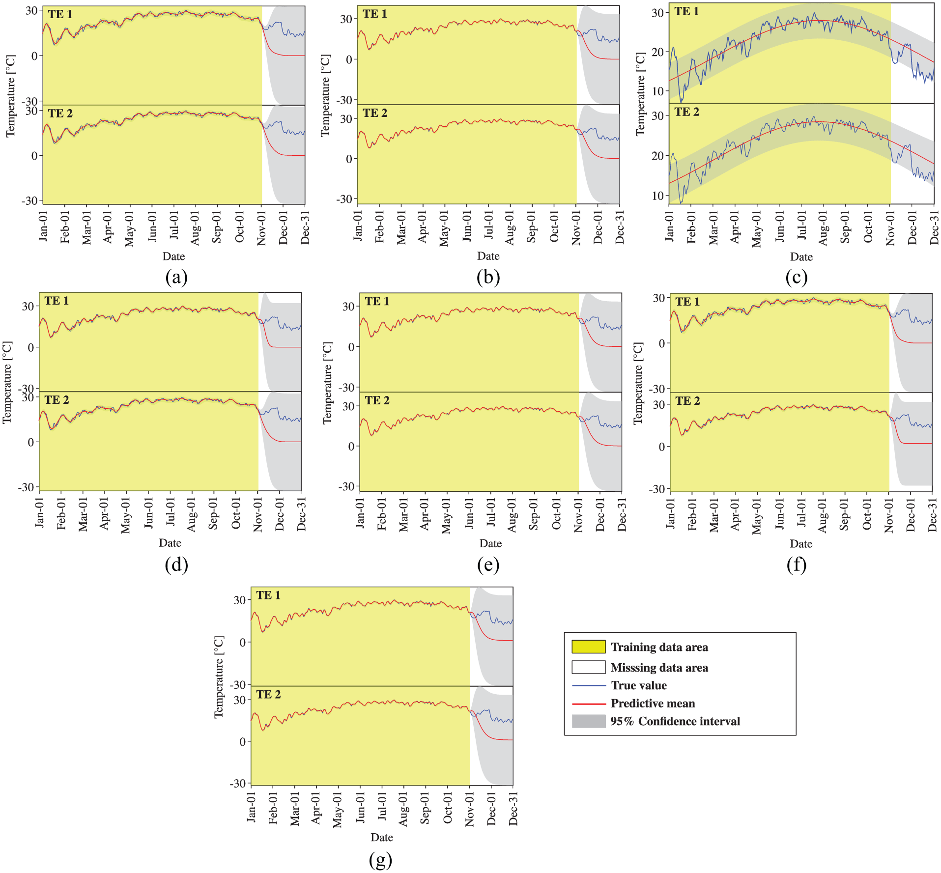
Temperature data reconstruction by MTGPM with different covariance functions (Case 5): (a) SE, (b) MA, (c) PE, (d) SE × PE, (e) MA × PE, (f) SE + PE, and (g) MA + PE.
Temperature data reconstruction by STGPM with different covariance functions (Cases 1–3): (a) SE, (b) MA, (c) PE, (d) SE × PE, (e) MA × PE, (f) SE + PE, and (g) MA + PE.
Temperature data reconstruction by STGPM with different covariance functions (Case 4): (a) SE, (b) MA, (c) PE, (d) SE × PE, (e) MA × PE, (f) SE + PE, and (g) MA + PE.
Temperature data reconstruction by STGPM with different covariance functions (Case 5): (a) SE, (b) MA, (c) PE, (d) SE × PE, (e) MA × PE, (f) SE + PE, and (g) MA + PE.
We first observe the reconstruction performance of MTGPM. It is found from Figure 5 that all constructed MTGPMs exhibit a good forecasting performance over the missing data segment except the one with the PE covariance function. This is because the PE covariance function can only feature PE variations in time series data. Given that the SHM data are likely to contain both PE and non-PE ingredients, the composite covariance functions that combine PE and other covariance functions would be more appropriate for formulating GPM. Figure 5 demonstrates that the “SE + PE” covariance function performs better than the SE covariance function, and the “MA + PE” covariance function is superior to the MA covariance function. It is also observed that the reconstruction capability of the MA covariance function–based MTGPM is higher than the SE covariance function–based one, and so are their hybrid covariance functions in combination with the PE covariance function. The reason explaining the greater reconstruction potentiality of MA and its related hybrid covariance functions is that the MA covariance function is better suited to the forecast of highly rough variations compared to the SE one. By comparing Figures 5 to 7, it is observed that the task similarity plays an important role in the reconstruction by MTGPM, and to be specific, higher task similarity gives rise to better reconstruction performance. Pearson’s correlation coefficient (PCC),
Subsequently, we turn to the observation of the reconstruction preformation of STGPM. As shown in Figures 10 to 12, the STGPM is unable to recover a large block of missing data. To be more specific, the STGPM preserves enough accuracy only for limited-step (one- or two-step) ahead reconstruction, and its reconstruction error becomes larger and larger with the increase in the time step of data reconstruction. Overall, the STGPM is not reliable for reconstructing a large amount of missing data. In light of the above observations, it can be concluded that the MTGPM presents an overwhelming superiority over the STGPM for reconstruction of SHM data, especially in the case with a large block of missing data.
Since the visual inspection of reconstruction performance of MTGPMs with different settings of covariance functions is subjective, two performance measures are adopted here to quantitatively assess the reconstruction capability. They are root mean square error (RMSE) and mean likelihood (ML). The expressions for these two metrics are given by
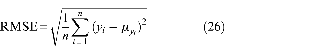
where
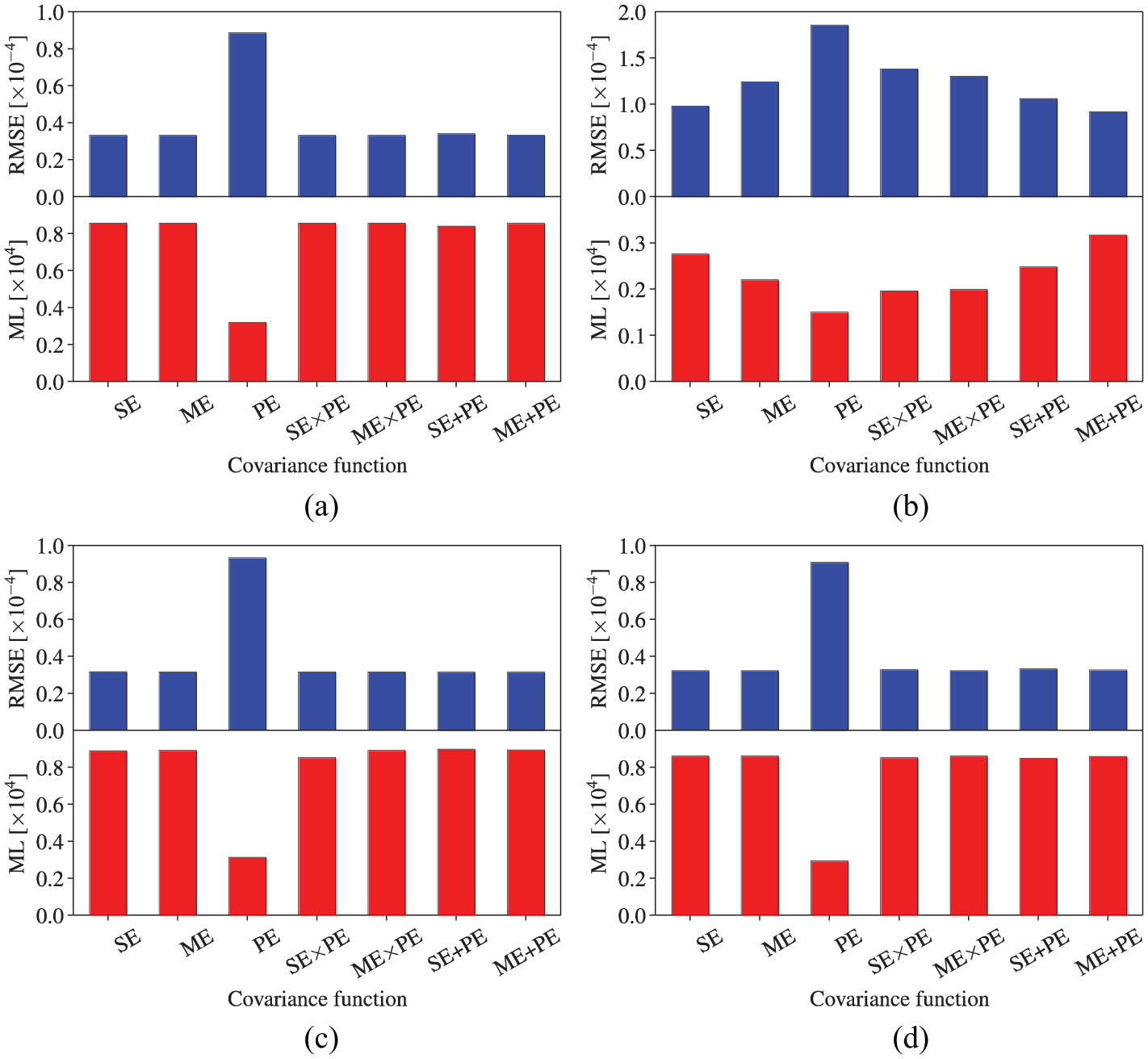
The reconstruction performance of MTGPMs using different covariance functions is compared in terms of RMSE and ML as shown in Figure 13. Note that Case 5 is not included here because, as mentioned before, MTGPM fails to favorably recover missing data when the missing data occur at the same time period for all tasks simultaneously. From Figure 13, several observations can be obtained:
Among the seven covariance functions, the PE one presents worst reconstruction performance. This is due to the fact that the time series data are not purely PE although they contain PE component.
The MA covariance function performs better than the SE covariance function. The higher reconstruction capability generated by the MA covariance function is attributable to its own feature that is unlike the SE one; the MA one does not impose strong assumption on the smoothness of time series data, allowing for a good description of highly rough variations in the SHM data.
The hybrid covariance functions created by sum operation, that is, “SE + PE” and “MA + PE,” provide greater reconstruction accuracy than the unblended SE and MA covariance functions, respectively. In contrast, the product operation-generated hybrid covariance functions (i.e. “SE × PE” and “MA × PE”) do not offer similar reconstruction capability to the sum operation-generated ones. The higher reconstruction capability of the sum operation-generated composite covariance functions than the product operation-generated ones might be explained by the fact that the SHM data are in general a sum of generic components such as seasonal and regression components, rather than a product of them.
Overall, the hybrid covariance function “MA + PE” leads to the best reconstruction capability among the seven covariance functions studied.
Performance assessment of MTGPM for temperature data reconstruction: (a) Case 1, (b) Case 2, (c) Case 3, and (d) Case 4.
Reconstruction of acceleration measurements
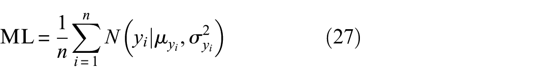
The acceleration data are used to further examine the reconstruction performance of the proposed Bayesian MTL methodology. Likewise, acceleration measurements collected from three accelerometers are considered here. In particular, the three target accelerometers associated with channel labels 07, 08, and 09 at the elevation of 228.50 m (Figure 2) are selected, which are denoted as “AC 1,”“AC 2,” and “AC 3,” respectively, for demonstration convenience. Figure 14 shows acceleration data collected from the three target accelerometers over 60 s. The PCCs between “AC 1” and “AC 2” and between “AC 1” and “AC 3” are
Acceleration monitoring data.
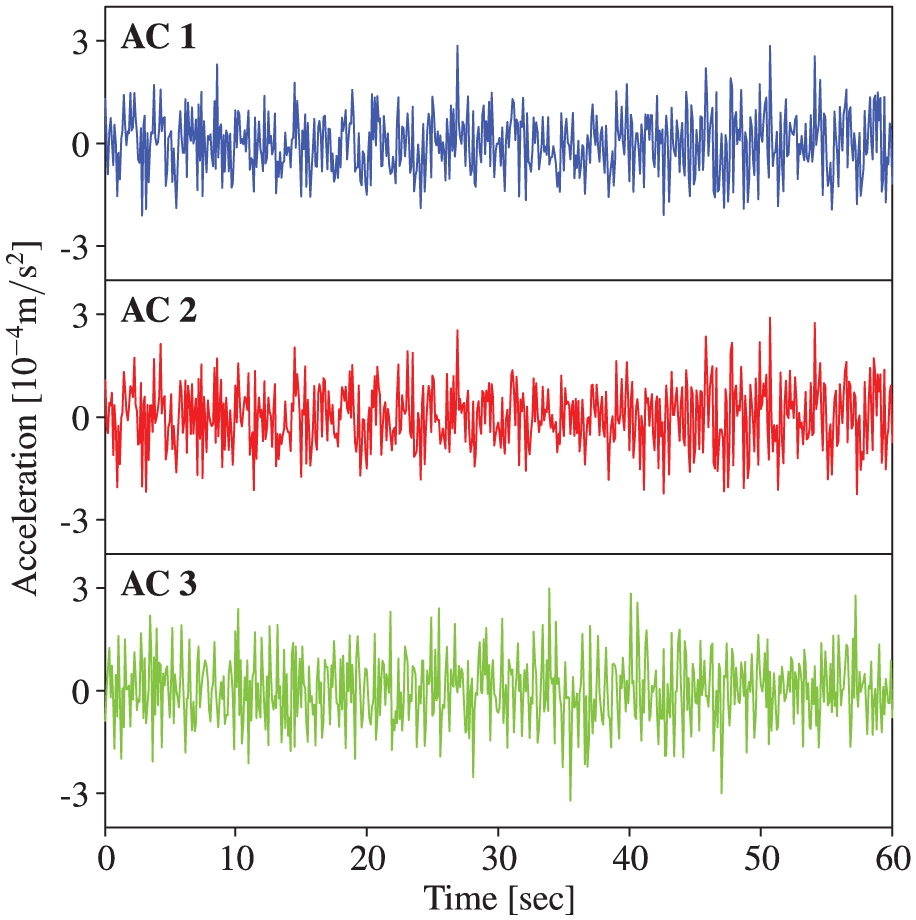
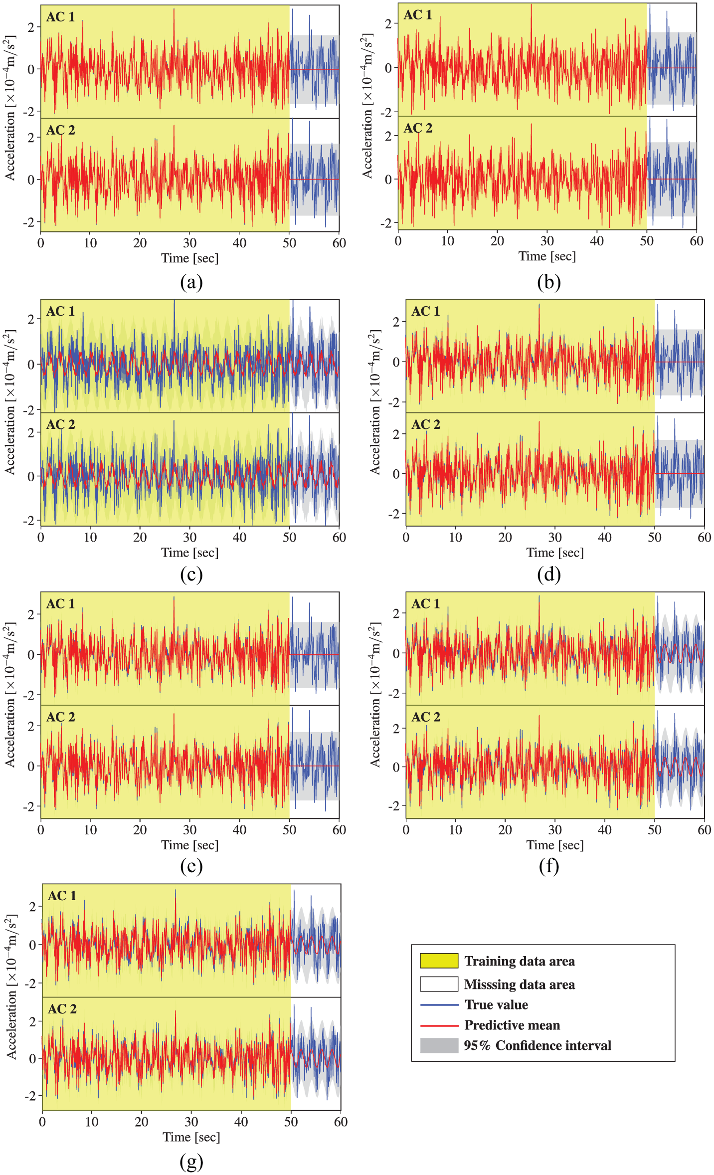
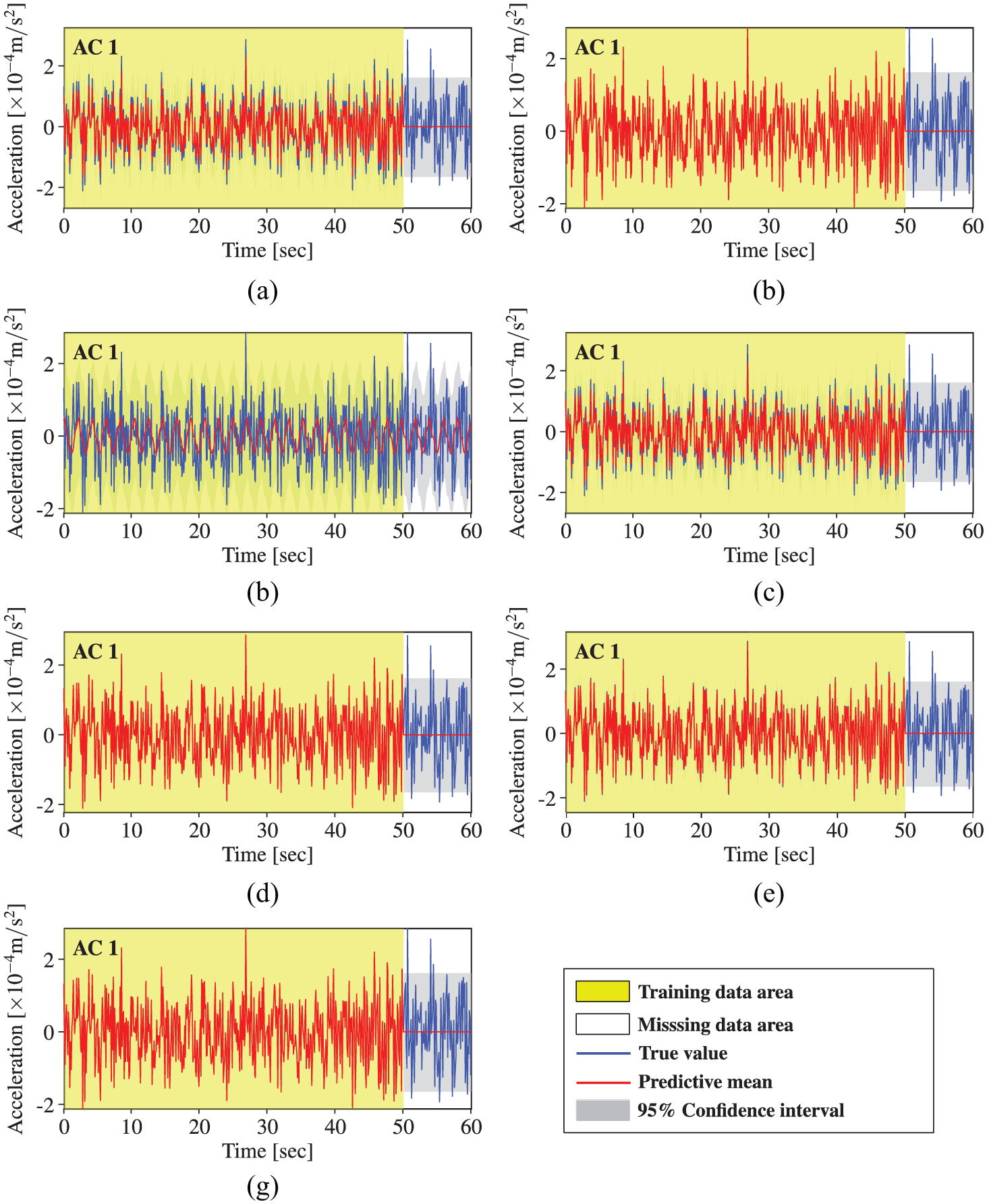
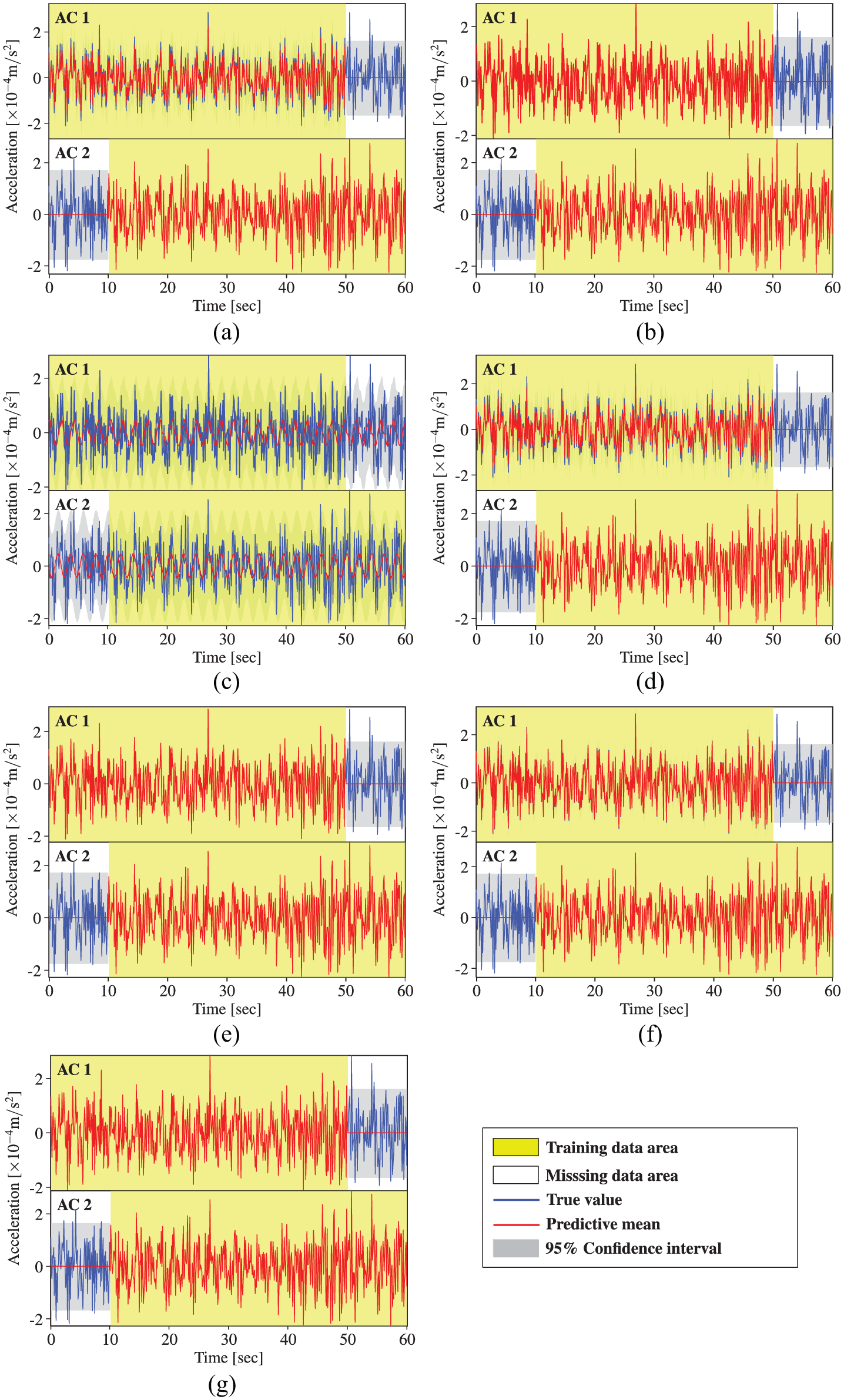
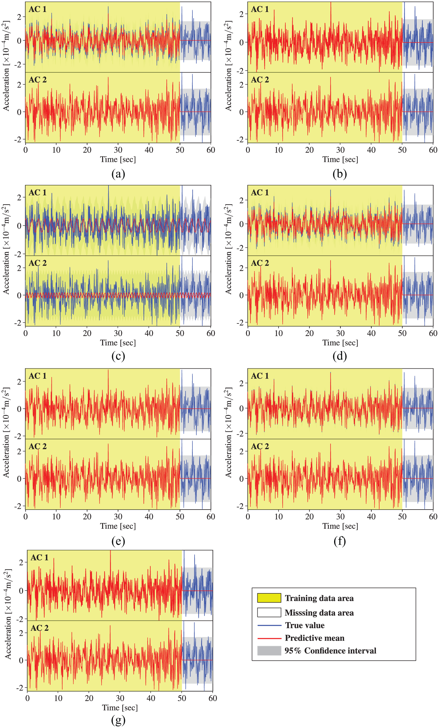
Like the temperature data case, one-sixth of the total acceleration data from one accelerometer serves as the missing data, that is, 10 s acceleration measurements in total is to be recovered. Then, MTGPM and STGPM are utilized to recover the missing data for each case mentioned in the above section, respectively. The data reconstruction results of MTGPM are shown in Figures 15 to 19, and those of STGPM are shown in Figures 20 to 22. The reconstruction performance of MTGPMs using different covariance functions for Cases 1–4 is quantitatively expressed in terms of RMSE and ML as shown in Figure 23. From Figures 15 to 23, the following observations are obtained through comparison with the temperature measurement cases:
It is confirmed again that the MTGPM exhibits better reconstruction performance than the STGPM. The higher the task relatedness, the higher reconstruction capability the MTGPM maintains.
Similarly, the MTGPM with the PE covariance function alone shows worst reconstruction performance. This can be illustrated by the incompatibility between the PE covariance function–based MTGPM prediction cures and the acceleration time series data. The former presents a strictly PE pattern, whereas the latter does not.
Likewise, the acceleration measurement cases also corroborate that the MTGPM using all three tasks together does not maintain a better reconstruction performance than that using only the two most related tasks. MTGPMs, no matter what covariance function is used, fail to favorably restore the missing data when all the tasks suffer from missing measurements over the same time.
Unlike the temperature measurements, the hybrid covariance functions do not show an advantage over the unblended ones in reconstructing missing acceleration data for all five cases. Specifically, the hybrid and uncombined covariance functions except the PE one show almost the same performance for Cases 1, 3, and 4, but for Case 2, the hybrid covariance function “MA + PE” still owns the best reconstruction capability among the seven covariance functions under investigation. Therefore, the hybrid covariance function “MA + PE” can be considered as an optimal choice in the proposed Bayesian MTL–based methodology for reconstruction of missing SHM data.
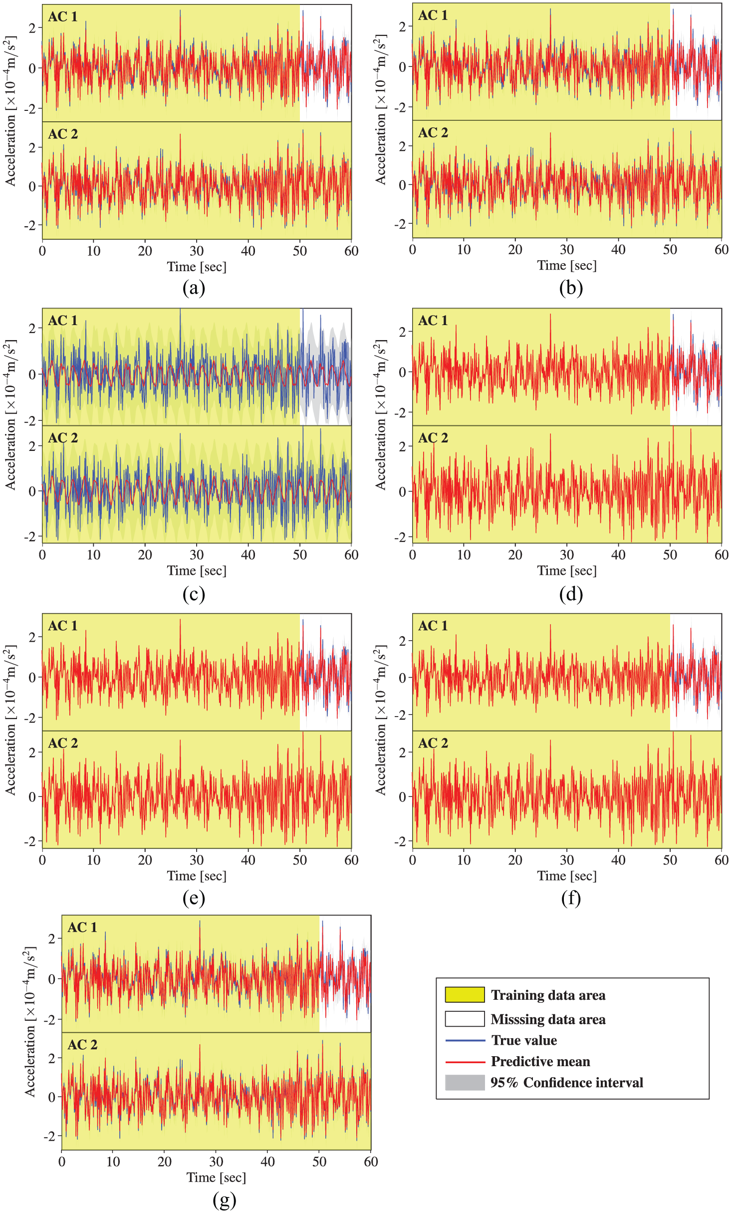
Acceleration data reconstruction by MTGPM with different covariance functions (Case 1): (a) SE, (b) MA, (c) PE, (d) SE × PE, (e) MA × PE, (f) SE + PE, and (g) MA + PE.
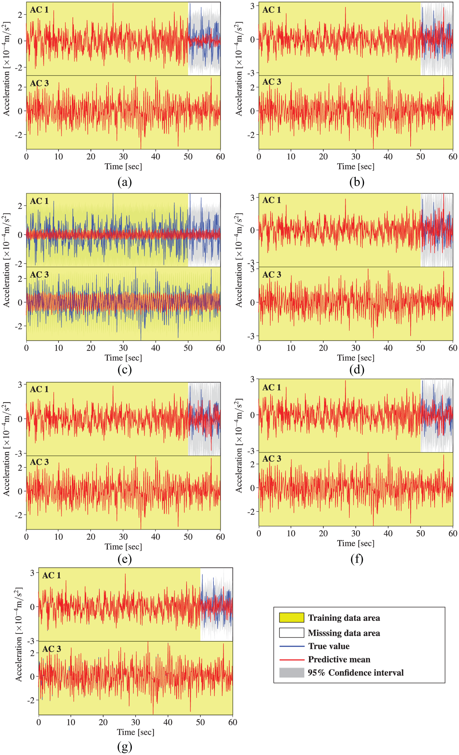
Acceleration data reconstruction by MTGPM with different covariance functions (Case 2): (a) SE, (b) MA, (c) PE, (d) SE × PE, (e) MA × PE, (f) SE + PE, and (g) MA + PE.
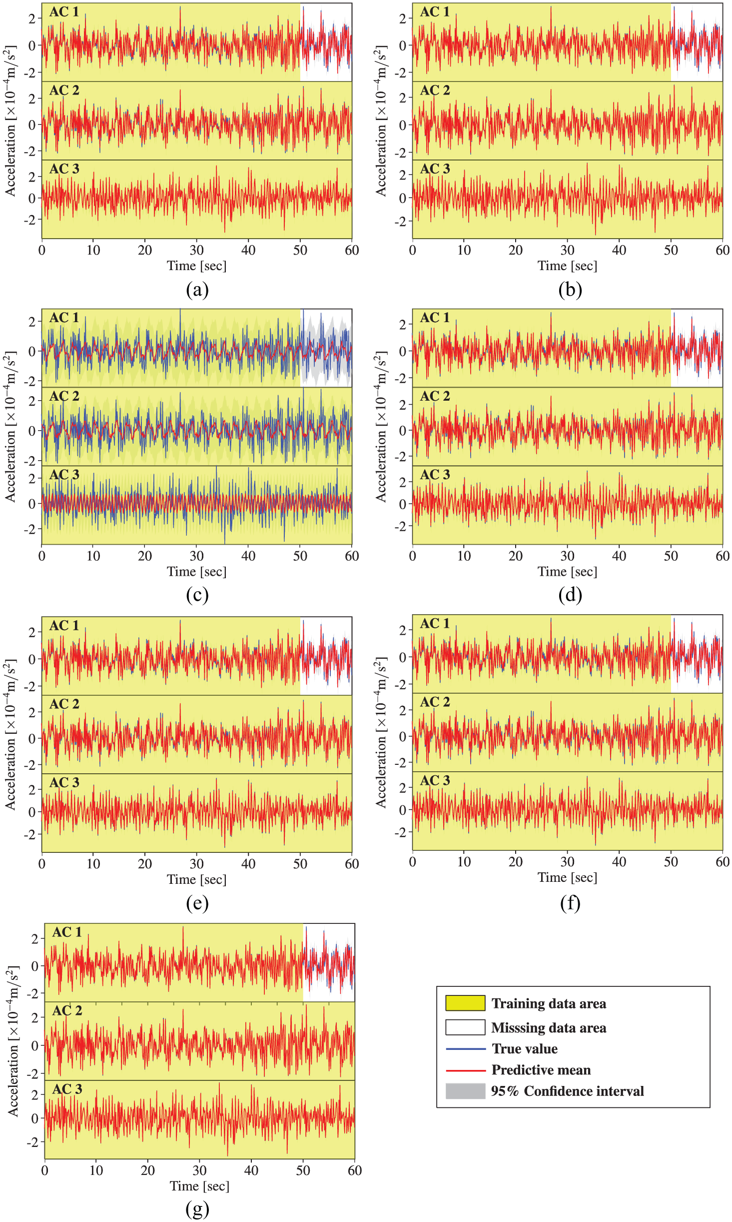
Acceleration data reconstruction by MTGPM with different covariance functions (Case 3): (a) SE, (b) MA, (c) PE, (d) SE × PE, (e) MA × PE, (f) SE + PE, and (g) MA + PE.
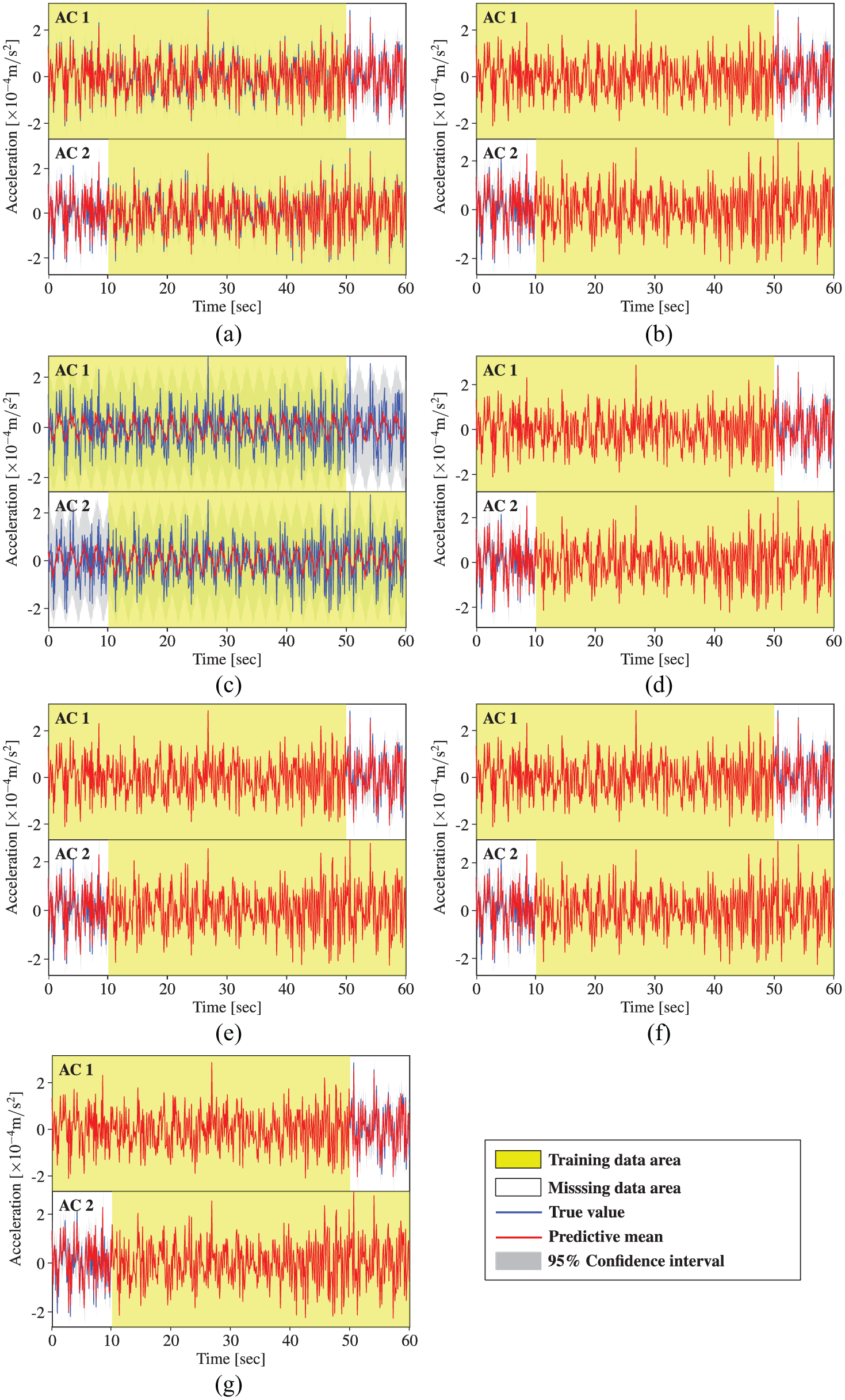
Acceleration data reconstruction by MTGPM with different covariance functions (Case 4): (a) SE, (b) MA, (c) PE, (d) SE × PE, (e) MA × PE, (f) SE + PE, and (g) MA + PE.
Acceleration data reconstruction by MTGPM with different covariance functions (Case 5): (a) SE, (b) MA, (c) PE, (d) SE × PE, (e) MA × PE, (f) SE + PE, and (g) MA + PE.
Acceleration data reconstruction by STGPM with different covariance functions (Cases 1–3): (a) SE, (b) MA, (c) PE, (d) SE × PE, (e) MA × PE, (f) SE + PE, and (g) MA + PE.
Acceleration data reconstruction by STGPM with different covariance functions (Case 4): (a) SE, (b) MA, (c) PE, (d) SE × PE, (e) MA × PE, (f) SE + PE, and (g) MA + PE.
Acceleration data reconstruction by STGPM with different covariance functions (Case 5): (a) SE, (b) MA, (c) PE, (d) SE × PE, (e) MA × PE, (f) SE + PE, and (g) MA + PE.
Performance assessment of MTGPM for acceleration data reconstruction: (a) Case 1, (b) Case 2, (c) Case 3, and (d) Case 4.
Conclusion
A new methodology for recovery of missing SHM data using Bayesian MTL has been proposed in this article. It is a model-free approach, which does not rely on the FE model and thus is preferable for restoring site-specific monitoring data. Specifically, the Bayesian MTL–based methodology is formulated to model multiple tasks collectively via a multivariate GP prior, which results in an MTGPM enabling the characterization of correlation among tasks, and the constructed MTGPM is executed to recover the missing data by invoking the shared information across tasks. The use of task relatedness encoded by MTGPM gives rise to better data reconstruction performance than learning each single task individually. The potentiality of the Bayesian MTL approach for missing data recovery becomes more pronounced when the training data are too limited to learn each underlying model separately or when there is a large block of missing data.
The reconstruction capability of the Bayesian MTL approach has been examined by using the real-time temperature and acceleration monitoring data acquired from a high-rise structure. Its reconstruction performance is also compared with the conventional Bayesian STL approach. In recognizing that the covariance function might largely influence the modeling flexibility and expressive power of GPM, the performance of different kinds of covariance functions including unblended and composite ones in data reconstruction is investigated thoroughly. A total of seven covariance functions (SE, MA, PE, “SE × PE,”“MA × PE,”“SE + PE,” and “MA + PE”) are utilized to assess the reconstruction performance of both Bayesian MTL and STL approaches under various missing data scenarios with different task combinations. The results indicate that the proposed Bayesian MTL–based methodology provides an excellent performance for data reconstruction, whereas the conventional Bayesian STL approach is not reliable to restore the missing data in some cases. It is also revealed that the covariance function plays an important role in missing data reconstruction by the Bayesian MTL–based methodology, and among the seven covariance functions, the hybrid covariance function “MA + PE” gives the highest reconstruction capacity, especially for the temperature measurements. In summary, this study presents a novel approach for reconstructing SHM data based on Bayesian MTL with a multivariate GP prior and meanwhile offers useful guidance on the selection of an appropriate covariance function for missing data reconstruction.
Footnotes
Declaration of conflicting interests
The author(s) declared no potential conflicts of interest with respect to the research, authorship, and/or publication of this article.
Funding
The work described in this article was supported by a grant from the Research Grants Council of the Hong Kong Special Administrative Region, China (Grant No. PolyU 152767/16E) and a grant from the National Natural Science Foundation of China (Grant No. 51508144). This work was also supported by the Hong Kong Scholars Program (Grant No. XJ2016039) and by the Hong Kong Polytechnic University (Grant No. 4-ZZCE).