
Abstract
Leakage from water distribution systems is a worldwide issue with consequences including loss of revenue, health and environmental concerns. Leaks have typically been found through leak noise correlation by placing sensors either side of the leak and recording and analysing its vibro-acoustic emission. While this method is widely used to identify the location of the leak, the sensors also record data that could be related to the leak’s flow rate, yet no reliable method exists to predict leak flow rate in water distribution pipes using vibro-acoustic emission. The aim of this research is to predict leak flow rate in medium-density polyethylene pipe using vibro-acoustic emission signals. A novel experimental methodology is presented whereby circular holes of four sizes are tested at several leak flow rates. Following the derivation of a number of features, least squares support vector machines are used in order to predict leak flow rate. The results show a strong correlation highlighting the potential of this technique as a rapid and practical tool for water companies to assess and prioritise leak repair.
Keywords
Introduction and background
Leakage in water distribution systems
Water pipes are the primary method of transporting water to customers worldwide. Leaking pipes are an international problem and represent dangers to public health and the environment, as well as economic losses from non-revenue water. 1 As water discharges through a leak, acoustic sound in the water column and vibration on the pipe wall is created. Sensors (normally accelerometers or hydrophones) placed either side of the leak can record this leak signal. The signal is then cross correlated with finding the leaks’ location (known as leak noise correlation). A number of factors have been shown to influence a leak signal and therefore vary the efficacy of leak noise correlators. Some of these factors have been investigated in the literature, including leak flow rate, backfill, pipe material,2–4 among others. The leak’s vibro-acoustic emission (VAE) is determined by all of the aforementioned parameters and therefore it may be possible to use the leak signal to predict both the leak flow rate 2 and leak area. 5
A system that can accurately predict leak flow rate will provide water industry practitioners with a tool to assess and prioritise leak repair and develop to drive down sustainable economic levels of leakage (SELL) (whereby the cost of repair should be lower than the cost of not repairing the leak 6 ). Butterfield et al. 2 developed a method to predict leak flow rate using the signal root mean square (RMS). A similar method was proposed for leaking gas pipes by Chen et al. 7 and Kaewwaewnoi et al. 8 These studies however only investigated a single hole size. Sun et al. 5 presented a study whereby the classification of different round hole diameter leaks on gas pipes using acoustic emission sensors was investigated and then classified using support vector machines (SVM). Despite the use of classification/prediction-based algorithms common in other disciplines (e.g. speech recognition), there are no robust techniques to predict leak flow rate on water distribution pipes using VAE-based measurements that are actively being used by water industry practitioners.
The aim of this article is to derive a method for predicting leak flow rate using VAE with no prior knowledge of leak size. In addition, the VAE will be explored to determine the potential for independent determination of leak diameter. A data-driven theory and an intelligent system to predict leak flow rate using least squares support vector machines (LS-SVM) is demonstrated in this article.
Feature extraction of leak signals
The use of classification or predictive machine learning algorithms involves using a number of features, which can be divided into time and frequency domain and time–frequency features. As leak VAE signals are non-stationary,9,10 approaches with good representation of non-stationary signals in both time and frequency domains could provide informative features. Empirical mode decomposition (EMD) is an adaptive time–frequency technique and has been shown to provide good estimates of time–frequency signals 11 and therefore may provide the required time–frequency resolution for leak signal feature extraction.
EMD breaks down a signal into different intrinsic mode functions (IMFs) which represent a different frequency content of the signal. The EMD method as a process of sifting is described below:
Find extrema of signal
Find lower and upper signal envelopes connecting the minima (cf. minima) and maxima (cf. maxima),
Calculate the signal mean between upper and lower envelopes,
Subtract the calculated mean to obtain ‘modulated oscillation’,
12
Apply stopping criteria.
12
If
Continue sifting until IMF calculated in step 5 becomes a monotonic function.
EMD has been used to successfully extract signals in noisy environments. 13 As leak signals on plastic pipe generally have a low signal to noise ratio, 14 EMD is likely to be particularly useful.
EMD alone suffers from a mode mixing problem due to IMF rectification and a signal may be separated into the same IMFs 15 resulting in inaccurate measurements. Huang et al. 16 suggest mode mixing could lose physical meaning of the signal as well as aliasing in time–frequency domains. This problem can be resolved by overcoming signal intermittency, 15 leading to the development of ensemble empirical mode decomposition (EEMD) by Wu and Huang. 15 Essentially, EEMD decomposes the signal via the EMD method, but during each decomposition process, Gaussian white noise of finite amplitude is added to the signal

where
As the additive noise is different for all decomposition levels, no mixing occurs. 17 Due to the higher accuracy in generating representative IMFs, EEMD is used in this study instead of standard EMD. A similar method was proposed by Si et al. 18 who used EEMD to decompose signals into IMFs with different energy for classification with LS-SVM.
Studying just one hole size, the RMS of leak signals has also been shown to effectively describe leak flow rate in plastic water pipe by Butterfield et al.
2
and in gas pipes by Chen et al.
7
EMD-based decomposition was used by Sun et al.
5
in combination with the signal RMS to classify the aperture of leaks in gas pipes, finding that the RMS of individual IMFs, produced from EMD provided good separation between circular holes in gas pipes of different diameters. RMS features can be used to characterise continuous vibration signals, with the RMS value representing the energy of the signal at that point in time
5
and could therefore be a good feature in predicting leak flow rates. The RMS of each decomposed IMF containing

The concept of Shannon entropy was introduced in order to characterise system complexity where more random, discorded systems have higher information entropy. Sheng et al. 19 used local mean decomposition followed by Shannon entropy and SVM in order to classify bearing running state. Sun et al. 5 also used the Shannon entropy of individual IMFs following EMD to recognise leak apertures.
Frequency domain features such as the fundamental frequency has been shown by Prime and Shevitz 20 to shift depending on whether or not a beam is cracked using accelerometers. Other frequency domain methods such as the maximum and mean dB of a signal’s power spectral density (PSD) was reported by Chen et al. 7 as a good descriptor of pin hole leaks in gas pipes. Based on the above review of the literature, the following features were used to predict leak diameter: RMS of IMFs following EEMD, Shannon entropy of each IMF following EEMD, Shannon entropy of the raw signal and RMS of the raw signal. In addition to the aforementioned features, standard metrics of mean dB of the PSD, maximum dB of the PSD, minimum dB of the PSD, standard deviation, signal power, fundamental frequency, spectral flux, kurtosis, skewness and crest factor were also included.
Redundant features can increase computational cost and the possibility of overfitting so need to be removed. A variety of methods exists for subset selection and has been reviewed by numerous authors.21,22 Brute force methods involve assessing all input combinations and then identifying the subset which provides the greatest accuracy but can have high computational cost, and there is a possibility of overfitting. So called ‘greedy methods’ include forward selection (‘forward search algorithm’) is a more conventional feature selection algorithm. Forward feature selection methods involve measuring validation error, and the best individual feature is identified. The best subset of two components is then found and continues finding the best combination of features.
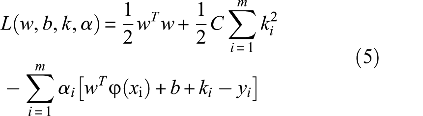
Least Squares-Support Vector Machines
SVM provide a method for solving classification problems with nonlinearity and pattern recognition 23 and has had some uses in leak detection. 24 However, SVM models involve complex quadratic programming problems 25 and are known to take a long time for training. 23 LS-SVM overcome the problems of SVM, whereby a number of linear equations are solved rather than quadratic equations.23,26 LS-SVM is therefore more optimal at solving non-linear systems, performing with higher accuracy. 18
LS-SVM have been shown to be successful at predictive problems, such as identification of cracks in images, 27 the characterisation of cracks in conductive materials 25 and faults in complex non-linear systems. 28 In the context of acoustic-based measurements, Shen et al. 23 used LS-SVM and wavelet packet decomposition of acoustic emission signals to classify the state of pressure vessels. There is no known use of LS-SVM in the context of leak detection; therefore, this study represents the known first application of this model to pipe leakage with VAE.
The LS-SVM algorithm has been described by Si et al.
18
and Chelabi et al.,
25
following the theory by Suykens and Vandewalle
26
and is described here for the completeness.
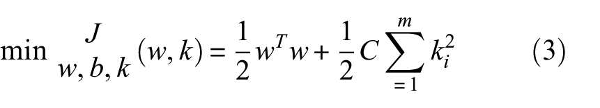
where

where
where
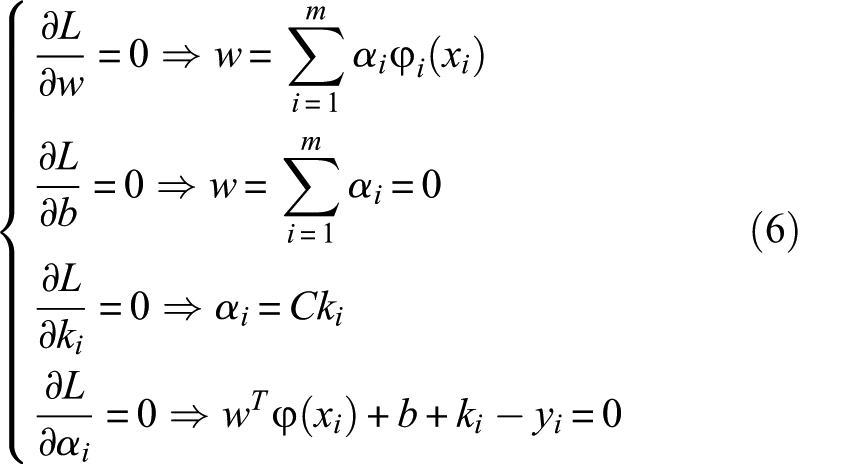
It is therefore possible to write a solution to a set of linear equations,
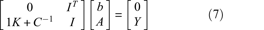
where

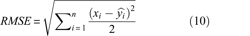
It is now possible to derive the regression function for the LS-SVM algorithm
It is necessary to ‘tune’ the hyper-parameters (γ and σ) in LS-SVM, and this was done by the leave-one-out method. 30
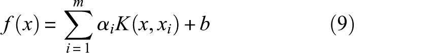
The model performance can be assessed through using the root mean square error (RMSE) and is a common parameter for assessing model performance. 31 As the RMSE shows the residual error, it provides a good estimate of the difference between the LS-SVM predicted values and the actual values. 32 RMSE can be described as
where
Methodology
Experimental methods
A series of tests was conducted on the novel, state-of-the-art leaks in viscoelastics (LIVE) pipe rig at the University of Sheffield, UK (Figure 1(a)) which was designed specifically for this study to minimise the possibility of signal reflections from other sources (e.g. the number of valves, fittings, bends were limited). The rig consists of approximately 26-m-long pipe loop with a 63-mm outer diameter 12-bar rated medium-density polyethylene (MDPE) pipe. Water is supplied from an upstream reservoir (0.95 m3 volume) by a 3.5-kW (Wilo, Burton Upon Trent, UK) MVIE variable speed pump set at 15 r/min. Water then passes a magnetic flow meter (Flow Systems 91DE) measuring system flow rate upstream of the leak. Two pressure sensors (Gems Plainville 2200) measure system pressure upstream and downstream of the leak at a sampling rate of 2000 Hz.
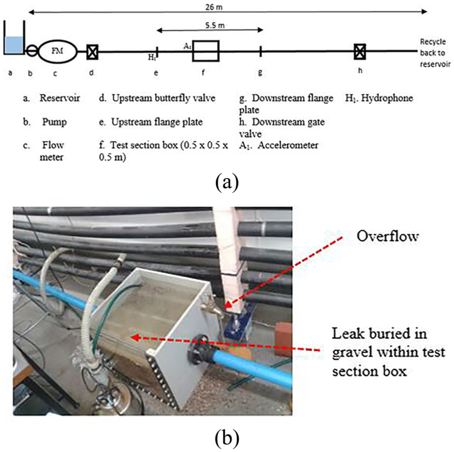
(a) Schematic of the LIVE pipe rig. Not to scale. Adapted from Butterfield et al. 3 and (b) picture of buried leak.
A removable 5.5-m ‘test section’ is located in the middle of the pipe. The test section allows for the alteration of leak size when the hole test section is replaced. This section of pipe is removed and reattached to the main pipe rig at two flange plates located at both ends of the test section. The test section is supported by the two flange plates, while the main pipe rig is supported using MDPE pipe clips at various points along the pipe rig. Circular holes of four different diameters (3.5, 4.5, 5.5 and 6.5-mm nominal diameter) were drilled through the pipe wall of four different test sections. Each drill bit was passed through the hole three times in order to reduce swarfs surrounding the hole. The test section passes through a rectangular box measuring 0.5 × 0.5 × 0.5 m3 and was filled with 5–12-mm diameter pea gravel backfill (Figure 1(b)), in accordance with British Standards 33 for backfill of plastic pipe and therefore represents a standard external porous media. The wavespeed in the pipe rig is estimated to be 347 m/s using theoretical calculations. 34
Initially, the system characteristics were measured with no leak in place to generate data on background noise. The leak VAE measurements were then taken from the pipe rig at consistent pressure heads and leak flow rate adjusted by turning the downstream gate valve. Tests were conducted leak flow rates of (1) 39–40 l/min, (2) 44–45 l/min, (3) 47–48 l/min, (4) 49–51 l/min and (5) 56–57 l/min. A wide range of leak flow rates can occur in real water distribution pipes, but in this study, these leak flow rates were chosen due to the experimental limitations of the pipe rig.
Signal processing and feature extraction
Leak signals were recorded using a hydrophone (Bruel and Kjaer type 8103, 50 × 9.5 mm2), placed 2.25 m from the leak. An accelerometer (393B12; PCB Piezotronics, Depew, NY, USA; sensitivity: 10 V/g) was placed approximately 30 cm away from the leak. Both sensors were sampled at 2500 Hz. The sensors were powered by a current source unit (Dytran Instruments type 4102C). Signals were then passed through a 6-m integral cable to a two-channel CCLD conditioning amplifier. Signals were processed in MATLAB and filtered using a fourth-order Butterworth bandpass filter at set points <10 Hz and >1000 Hz. A total of 20 samples were taken per leak flow rate and leak shape. About 60% of these samples were used for training of the data, and the remaining 40% used for testing (Figure 2). A total of 24 time, frequency and time–frequency domain features were extracted from the raw hydrophone and accelerometer signal, and these are listed in Table 1.
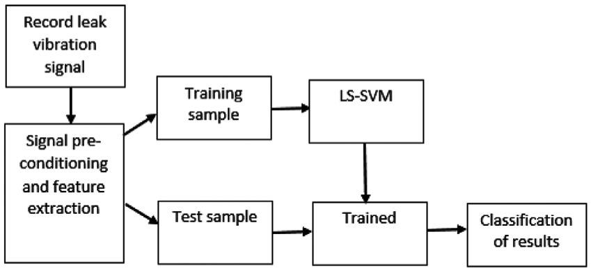
Process of signal processing, feature generation and results classification.
The features extracted from both the accelerometer and hydrophone signals.
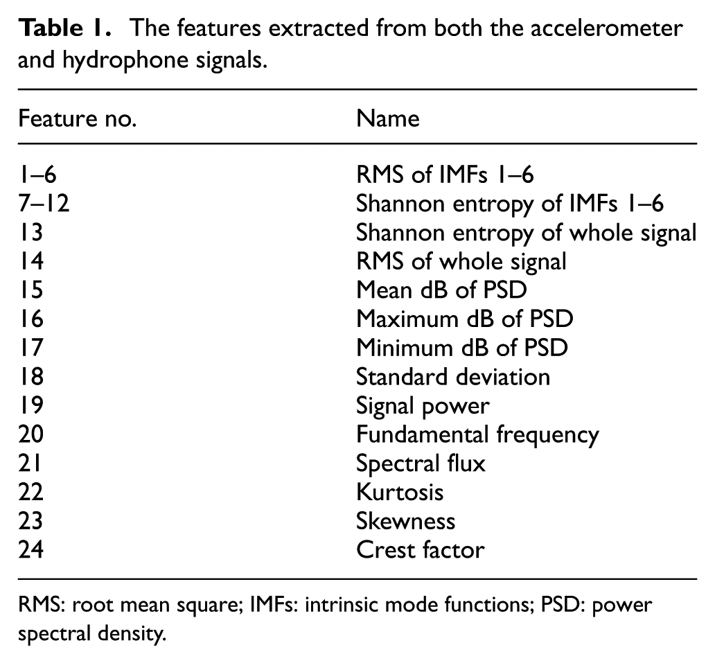
RMS: root mean square; IMFs: intrinsic mode functions; PSD: power spectral density.
Results
Leak signal characteristics
The frequency domain response of leak signals recorded with hydrophones following bandpass filtering are shown in Figure 3 for the low and high leak flow rates (39–40 and 56–57 l/min, respectively) for all hole diameters and is compared to the ‘no leak’ case. Background noise was defined as when the signal present in recorded leak signals is equal or less than the signal in the ‘no leak’ case and was found to be at frequencies <28 Hz. Signals for all hole diameters follow a similar spectral pattern, with the highest amplitude signals at the lower frequency range. A decline in amplitude at approximately 557 Hz occurs in the spectrums of all hole diameters. Increasing system pressure and thereby leak flow rate resulted in an increase in signal amplitude for frequencies in all hole diameters studied. However, it appeared easier to distinguish between leak flow rates at frequencies >207 Hz due to the wider separation between leak spectral patterns are these frequency ranges.
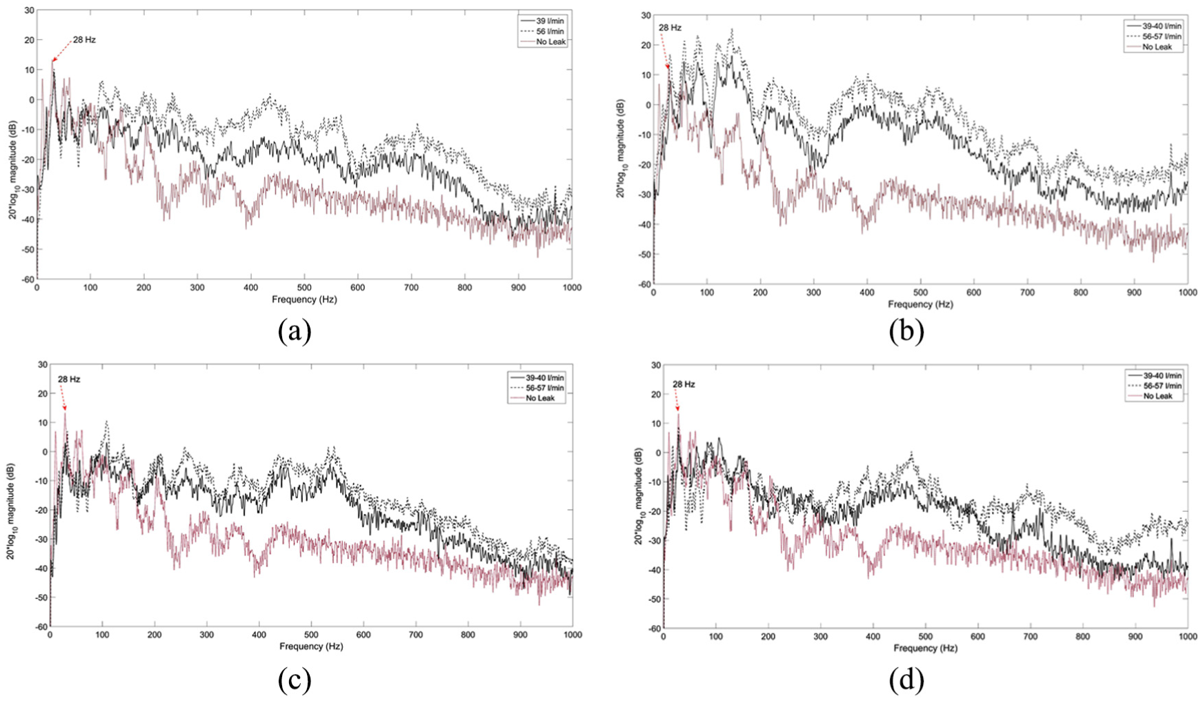
Frequency domain signals of round hole leaks of different diameter: (a) 3.5 mm, (b) 4.5 mm, (c) 5.5 mm and (d) 6.5 mm.
The resulting frequency spectrums for each hole diameter at 39–40 l/min are plotted together in Figure 4 for comparison. As they are all at similar leak flow rates, the effect of leak diameter can be isolated. Leak diameter appears to have no visible effect on the leak signal when the flow rate is kept consistent across hole diameters where a similar frequency and amplitude spectrum is observed. However, there appears to be some difference with 4.5 mm, which tends to be higher in amplitude and a different spectral pattern compared to the other three hole diameters, especially at frequencies 60–157 and 300–600 Hz.
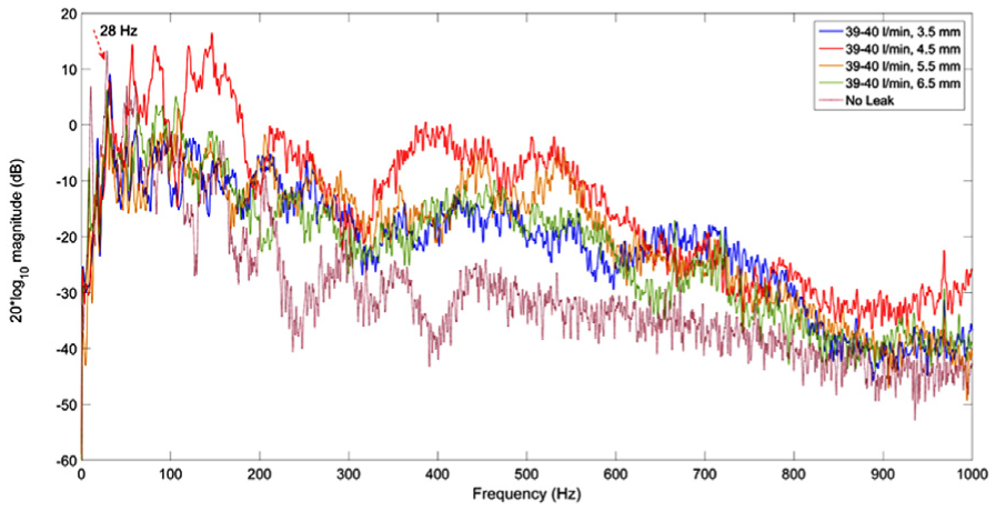
Frequency domain signals of round holes of different diameters at 39–40 l/min.
Data processing
Feature extraction
The research methodology presented in this study utilises 24 different features (Table 1). The measured signals shown in Figures 3 and 4 were subsequently decomposed via EEMD (described in section ‘Feature extraction of leak signals’) into individual IMFs. The corresponding first six IMFs and the Fourier transforms of these IMFs are shown in Figure 5(a) and (b), respectively. All IMF frequency components were found to be well below the pipe ring frequency (estimated to be in the region of 20 kHz for this pipe rig). The complexity of the leak signal is highlighted, in that the separate IMFs are related to different frequency components of the leak signal, with a decrease in frequency as IMF number increased. The EEMD decomposition identified leak signal in the region of 0–1000 Hz. The highest frequency components were identified in IMF1 and found to between 150 and 1000 Hz. However, these were distinctly low amplitude. Higher number IMFs were related to higher frequency, and in general, those IMFs > IMF1 were of greater amplitude compared to IMF1. However, the highest IMFs (IMFs 4–6) represent the lowest frequency components and are regarded as background noise (IMFs 4–6 are <28 Hz, and in accordance with Figure 3, this is equivalent to background noise).
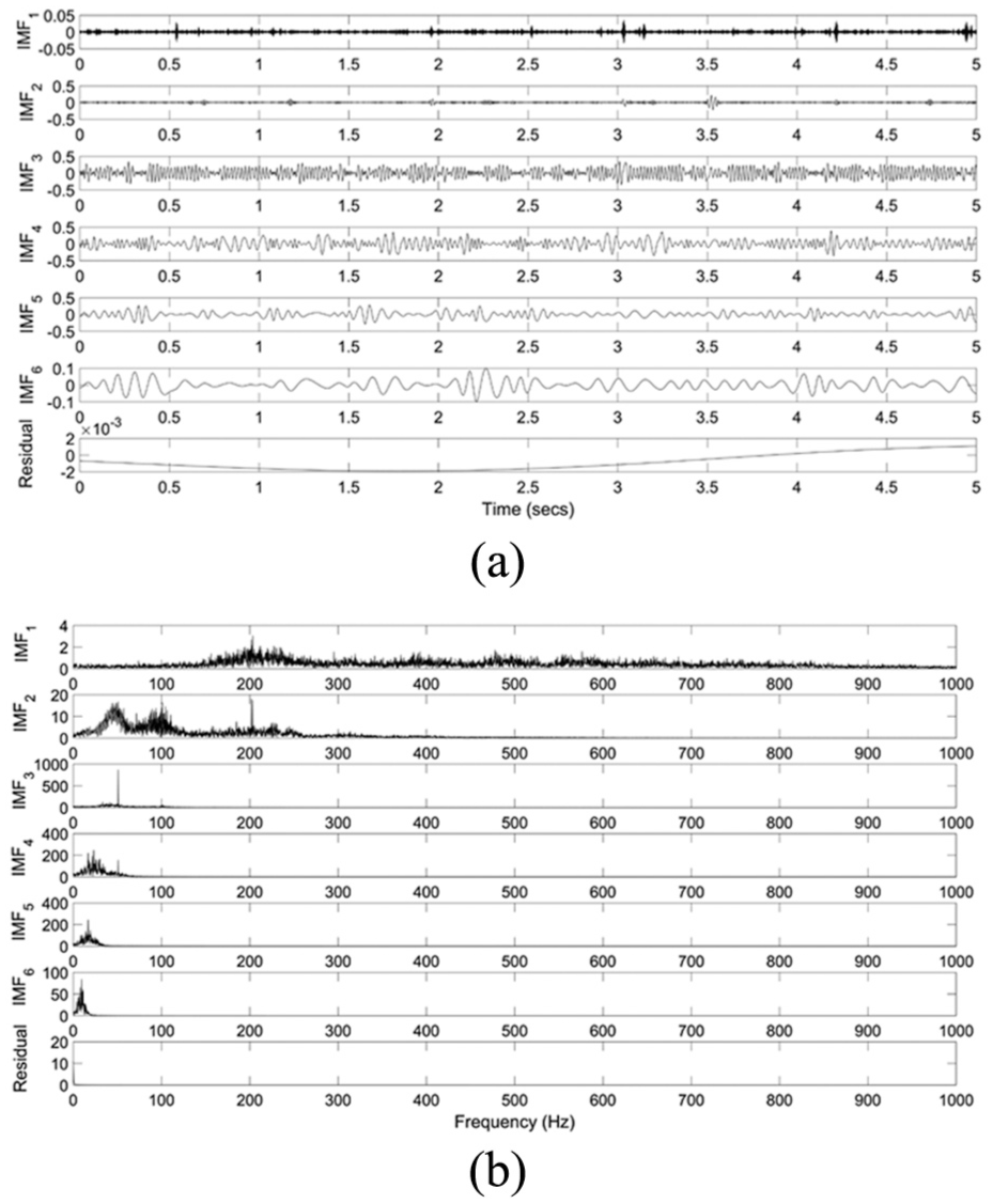
(a) IMF representation of EEMD decomposed signals and (b) a subsequent Fourier transform of each IMF. Example shown is the median leak flow rate leak flow rate (44–45 l/min).
Optimisation of model parameters
A total of 24 different features have been derived from the accelerometer and hydrophone signals. The most important features were selected using the ‘forward search algorithm’ (section ‘Feature extraction of leak signals’), eliminating redundant features, increasing the learning speed and prediction accuracy. The ability of the forward search to identify the most important features was determined by assessing the model output RMSE and this is shown in Table 2. It was found that the model would begin with high RMSE values and would decline as additional features were added systematically by the forward search algorithm. However, the model would reach a point where the addition of further features resulted in higher RMSE and therefore poorer model performance.
Feature selection and reduction in feature redundancy when predicting leak flow rate and leak area.
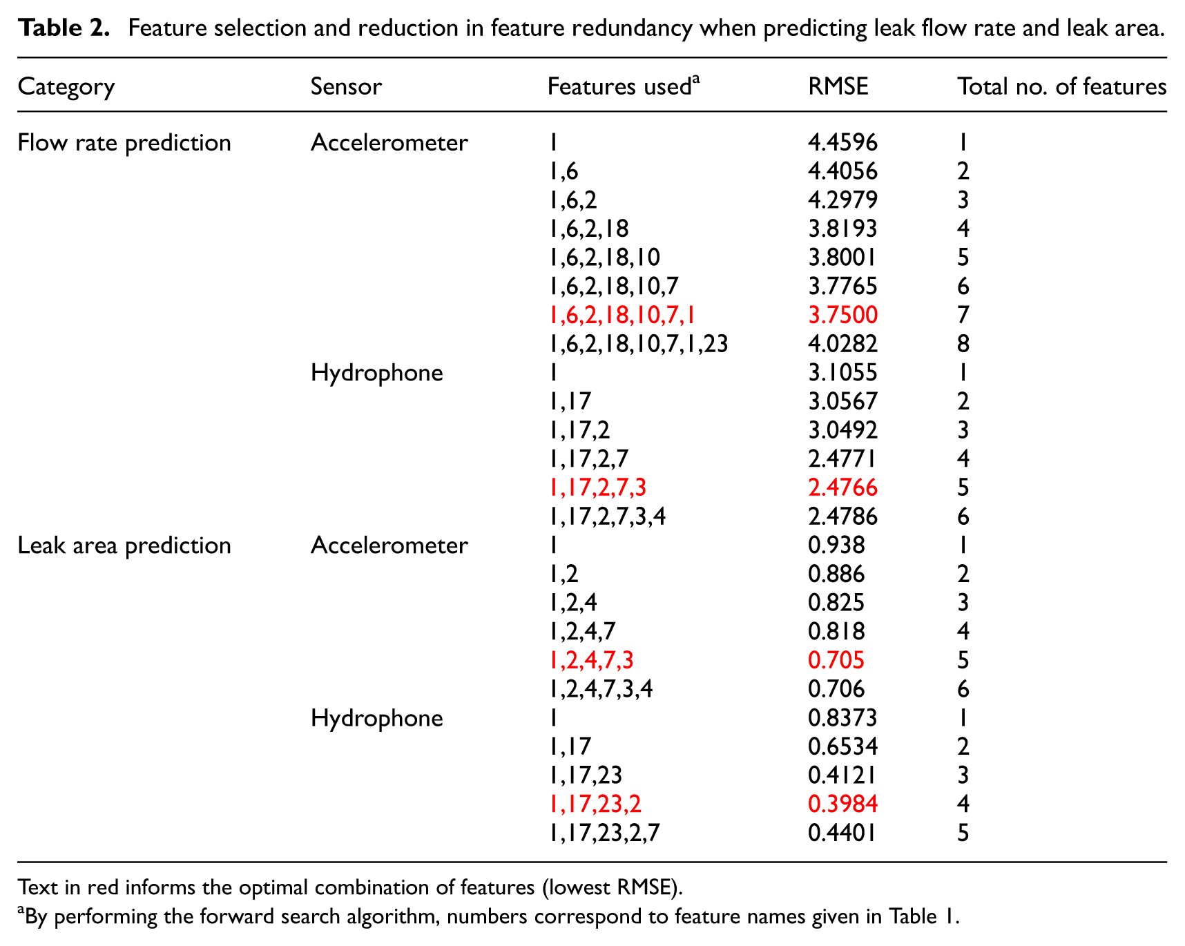
Text in red informs the optimal combination of features (lowest RMSE).
By performing the forward search algorithm, numbers correspond to feature names given in Table 1.
When predicting leak flow rate, the forward search identified five features using the hydrophones while seven features were identified using the accelerometers (Table 2). When predicting leak area, the forward search identified four features with the hydrophone and five features using the accelerometer. The output of the forward search algorithm suggested that the optimal combination or features differed depending on using hydrophones of the accelerometers and whether the model was chosen to predict leak flow rate or leak area. Generally, the most valuable features appeared to be those that represent time–frequency characteristics, and some common features were found to be useful for the model no matter how the model was adjusted or sensor choice (feature numbers 1 and 2).
Model training and testing
To assess the ability of the model to predict leak flow rate, the RMSE was used and is shown in Figure 6. When predicting leak flow rate, the results demonstrate that good performance can be achieved when using hydrophones to high accuracy with a low RMSE of 2.4766 (l/min) (Figure 6(a)). The output standard deviation was also calculated for each flow rate and found that the model performed better with lower standard deviations at the mid-range flow rates with standard deviations of 2.3, 1.4 and 1.6 at 44–45, 47–48 and 56–57 l/min, respectively. The prediction results were notably poorer at the extremities, with the lowest leak flow rate (39–40 l/min) and highest leak flow rates (56 l/min) demonstrating higher standard deviations of 2.5 and 2.7, respectively.
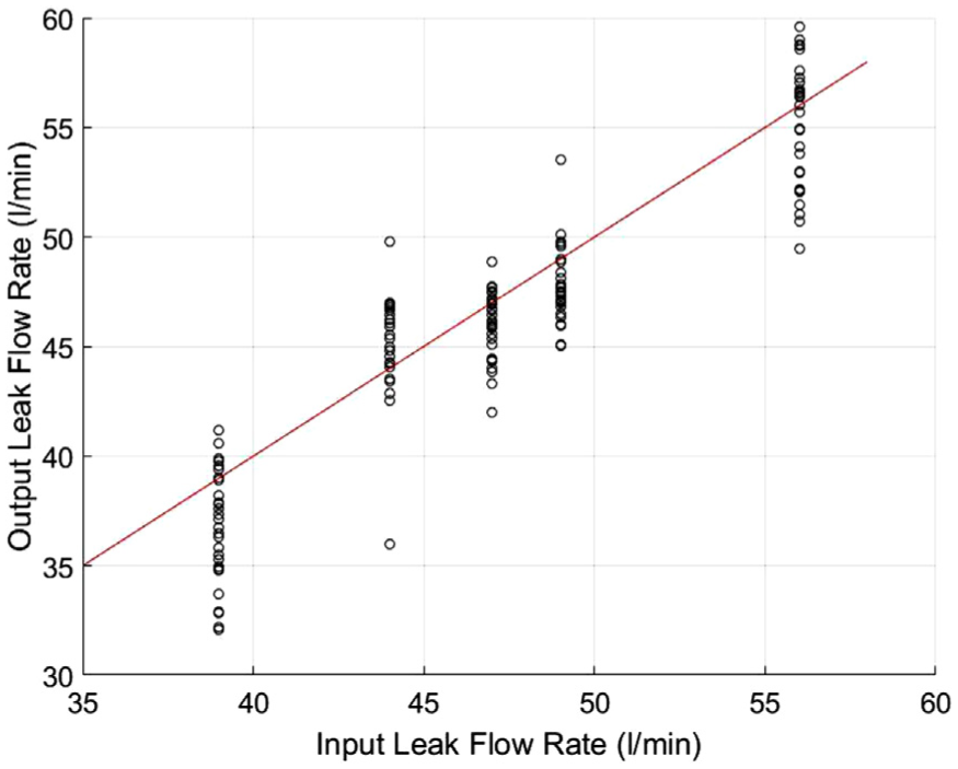
LS-SVM output results to predict leak flow rate using a hydrophone.
The data were reanalysed in order to predict leak area using hydrophones measurements. The actual versus output leak diameter is given in Figure 7. The hydrophone showed good prediction results with low overall RMSE (0.3984 mm). The best predictive performance came from using hydrophones at the lowest leak diameter of 3.5 mm. The resultant standard deviations for each leak diameter revealed better performance at 3.5 mm but poorer performance in predicting the 6.5 mm hole.
LS-SVM output results to predict leak area using a hydrophone.
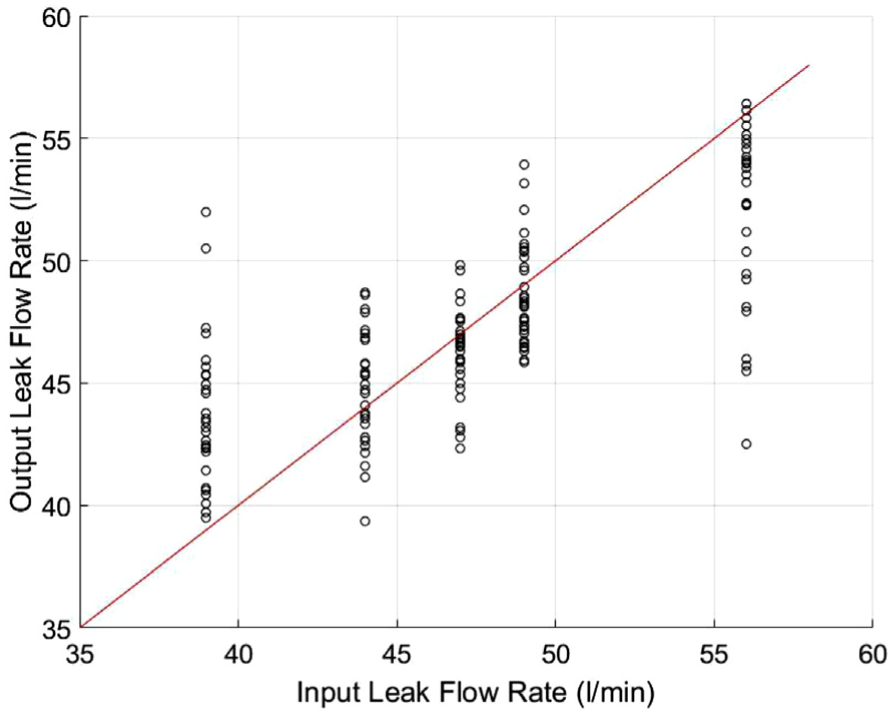
In order to assess the implications of using an alternative sensor, the measurements were repeated using an accelerometer. Figure 8 describes the actual versus output leak flow rates when predicting leak flow rate using accelerometers. It was found that, although the model could provide leak flow rate predictions using an accelerometer, these were significantly worse than when using the hydrophones (RMSE: 2.4766 and 3.7570 l/min for hydrophone and accelerometer, respectively) (Figures 6 and 8, respectively). Unlike with hydrophones, there was no observable trend in standard deviation – the mid-range flow rates gave high standard deviations comparable to the lowest and highest leak flow rates.
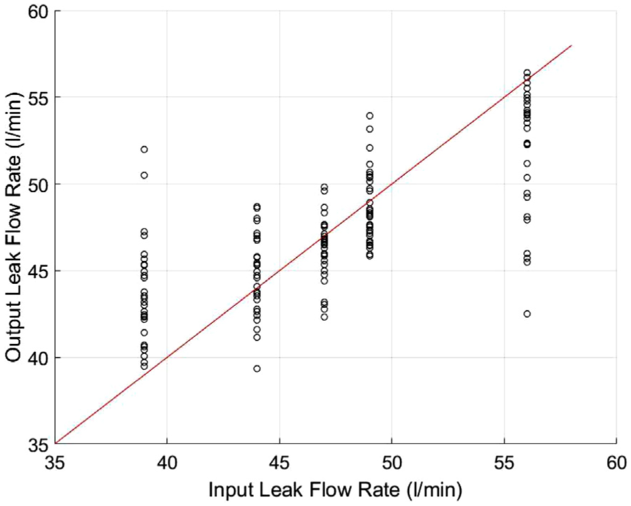
LS-SVM output results to predict leak flow rate using an accelerometer.
With the optimal model parameters chosen from the subset of features, it is possible to estimate the accuracy of the LS-SVM model quantitatively. Figure 9 demonstrates the accuracy of the flow and area prediction of the LS-SVM model at each leak flow rate and each leak diameter within ±10%. It was found that the optimum LS-SVM model provides excellent leak flow rate prediction results with the hydrophone data. Excellent prediction results were found at all leak flow rates, consistently achieving above >70% prediction accuracy (Figure 9(a)). Comparable to the results in Figure 6, greater prediction accuracy was found at the mid-range leak flow rates. The application of the model to accelerometer led to a reduction in prediction accuracy for all leak flow rates, reducing the accuracy of the model between 31.3% and 7%. On average, the hydrophone was found to accurately predict leak flow rate 15.9% more than the accelerometer.
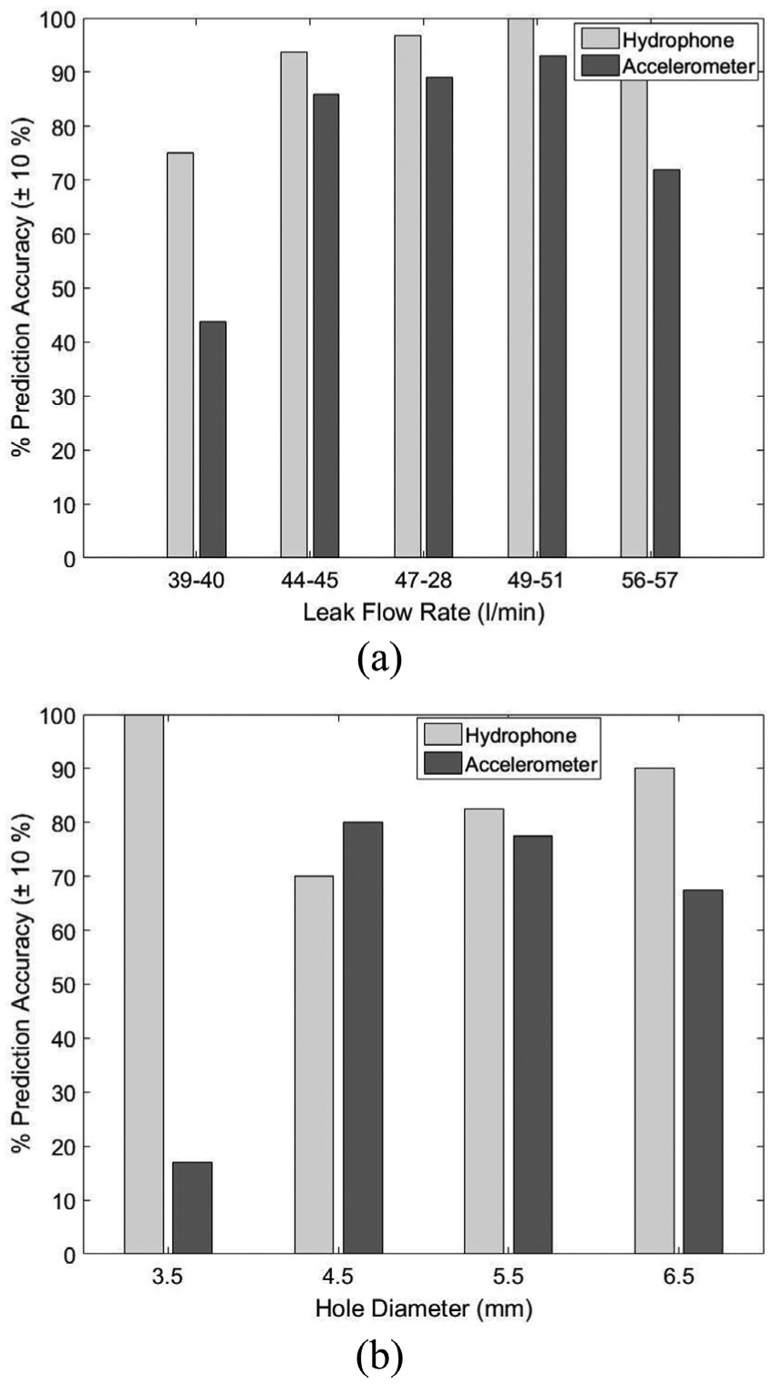
Accuracy of hydrophones in predicting (a) leak flow rate and (b) leak area within ±10% band.
Predictions of leak area within ±10% (Figure 9(b)) were also excellent with all area predicted >70% using hydrophones. Contrary to leak flow rate prediction, the area towards the extremities had the highest rate of prediction accuracy (100% and 90% prediction accuracy for 3.5 and 6.5-mm round holes, respectively). The use of accelerometer signals lead to a decrease in % accuracy when predicting leak area. The most significant difference in prediction appeared at 3.5 mm where the hydrophone was able to accurately predict leak area 100% of the time (±10%), whereas the accelerometer performed poorly only predicting the area of the 3.5-mm hole 17.5% (±10%). On average, the hydrophone predicting leak area 25.13% better than the accelerometer.
Discussion
The research presented herein aimed to derive a method to predict the flow rate of leaks in MDPE pipes using a LS-SVM on a novel experimental pipe rig where a unique data set was collected.
Leak characteristics
It was found that leak flow rate had a strong effect on the leak signal. Increasing leak flow rate led to an increase in amplitude of all frequencies greater than the background noise level (>28 Hz) for all hole diameters (Figure 3). However, there appeared to be clearer separation between leak flow rates at frequencies around >207 Hz. The observed increase in signal amplitude is coherent with other studies,2,35 and it is also likely that the higher flow rate leaks will be more easily identified than those with smaller leak flow rates 14 due to the increased signal amplitude.
When the leak flow rate was standardised, small differences in leak area were noted at the lowest leak flow rate with similar magnitude spectrums (Figure 4). At higher leak flow rates, the differences in leak area became more apparent, particularly at frequencies >600 Hz. Cassa and Van Zyl 36 and Ferrante 37 have shown leak area to be a key variable in defining the leakage behaviour.
However, there were noted differences in signal the 4.5-mm test results at both 39–40 and 56–57 l/min. These differences are more likely due to experimental features, such as the cutting process and localised material stresses 38 caused when drilling the leak holes. It is likely that limitations in the experimental design have led to changes in turbulence around the leak as the water jet discharges hole (possible due to the presence of swarfs during the drilling process). As turbulence around the leak hole is a strong parameter governing the leak signal, 39 it is important that any swarfs are either removed or standardised between studies. The differences in leak signal observed between hole size when the leak flow rate was standardised may also be due to changes in leak jet angle, which is strongly governed by pipe flow velocity and pressure head. 40
These results have shown that the effect of leak area will have little influence on the leak VAE signal (and therefore leak detection) at lower flow rates but is more important at higher leak flow rates.
Performance of the LS-SVM model
Following the derivation of a number of features, the LS-SVM model was used to predict leak flow rate despite changes in leak area. The model showed better leak flow prediction at the mid-range leak flow rates (Figure 6) with lower standard deviations and higher prediction accuracy. The model was able to predict mid-range leak flow rates to higher accuracy than at the extremities. This is possibly due to the fact that there is a greater population of data positioned within a smaller range of flow rates within the mid-range leak flow rates (minimum of 44 l/min and maximum of 51 l/min). However, at the extremities (39–40 and 56–57 l/min), there are fewer data points and therefore the model has a small proportion of data to train on.
Considering there is little difference between the magnitude spectrums when measuring leak area (Figure 4), surprisingly good prediction accuracy was also shown when predicting leak area, with lower standard deviations at the lower leak diameter and a slight increase trend in standard deviation as the hole size increased. This highlights the importance of deriving different features from the data set – it may be possible that a different set of features are able to describe leak area more than the relativity simple magnitude spectrum. The ability to independently predict either leak flow rate or leak area suggests that in future, a multivariate fitting process would be a profitable area of investigation.
Optimal feature selection
It was found that features relating to signal RMS were highly useful for predicting leak flow rate and leak area, whereby the RMS of IMF1, IMF2 and IMF3 were identified by the forward search algorithm as providing the optimal combination of features (Table 2). Signal RMS is likely a useful parameter as it has been shown to increase with leak flow rate.2,8,7 Interestingly, the model preferred to utilise features that are broken down by individual frequency bands rather than the RMS of the whole signal which was not favoured by the model. The fast Fourier transform (FFT) of each IMF has demonstrated that those IMFs > IMF3 represent the extremity of the signals lowest frequencies and represent the background noise (<28 Hz) identified by comparing the leak and no leak spectrums (Figure 3). As these higher IMFs represented the background noise, the model prefers to predict leak flow rate based on the RMS of parts of the signal relating solely to the leak signal and excludes background noise.
As the model favoured time–frequency domain representations of the leak signal, the efficacy of these features will become less useful when the sensor is positioned further away from the leak. A loss of higher frequency components and a general reduction in signal amplitude due to signal attenuation on the pipe wall and radiation into the surrounding media, 41 the leak has a low signal to noise ratio 14 and is difficult to distinguish from the background noise. Therefore, the features which are highly valued by this model will be reduced in efficacy as these features are only present in this study as the sensor was positioned close to the leak. It may then be more difficult to quantify leak flow rate using these features at greater distances from the leak, and it may be more valuable to use other features which are focussed around spectral shape as in reality it would be difficult to position a sensor next to a leak.
Sensor choice
It was found that hydrophones provided much better performance in predicting leak flow rate and hole area compared to accelerometers, with hydrophones achieving a much better RMSE and classification rate (Figure 6). This agrees with current understanding that hydrophones usually offer better performance for leak detection when compared with accelerometers.41,42 Improved performance using hydrophones may be due to the effect of a smaller effective bandwidth and higher signal coherence 41 when using hydrophones. As the accelerometer is placed on the pipe wall, it may be more susceptible to changes in ground conditions. While efforts were made to ensure that the ground conditions were standardised, the replacement of test sections resulted in the excavation of the pipe from the gravel backfill. The ground conditions have been shown to have a strong influence on the leak signal.3,4 Slight changes to the test conditions are possible through changes in loading, soil hydraulics and flow resistance which can have an influence on leakage dynamics. 43 As the accelerometer is in contact with the pipe wall, the effect of ground conditions may be more paramount and therefore may interrupt with the signal.
Wider context and industrial application
This study has managed to accurately predict the leak flow rate regardless of the leak area and with no prior knowledge of the leak area. However, in real water distribution pipes, it is unlikely that the leaks on plastic pipe would be perfect round holes of these given sizes; in fact, the majority of plastic pipe leaks occur due to joints contaminated during the pipe installation process. 44 Despite this, this research has established the first base case in leak flow rate prediction with the successful application of the LS-SVM model. However, classification of leak flow rates of different shapes and sizes represents a priority in any future work.
Excellent results using this LS-SVM model suggest that this is a suitable method in predicting leak flow rate area using hydrophone measurements for leaks in water distribution pipes. Any system that manages to predict leak flow rate will be advantageous to water companies, by prioritising leak repair and driving down SELL – repairing the bigger leaks first will save more water by fixing less leaks and costs savings through optimised allocation of company resources. Attempts were also made to predict leak area using the same model. As there is potential for contaminant ingress into water distribution systems through leaks, 45 level of contamination will involve the size of the leak area (among other factors such as driving force). 38 Therefore, a tool which provides the leak area will be useful in judging the risk of contamination due to ingress and therefore the threat to public health. The method can also be combined with existing leak noise correlation methods in order to provide both the leak flow rate and the leak’s location.
Conclusion
This article has categorically demonstrated that the leak flow rates in leaking MDPE pipes can be determined from VAE measurements without prior knowledge of leak area. High-quality experimental data from a specifically designed MDPE pipe rig were collected with hydrophones and accelerometers. Four separate test sections with different sized round holes were drilled, and system pressure was varied to alter leak flow rate.
The leak flow rate and leak area were found to both influence the leak spectrum. A total of 24 different features were derived from the raw signal and analysed via LS-SVM. It was shown that the signal contained sufficient information about the leak in order to accurately predict leak flow rate without prior knowledge of the hole area. It was also possible to accurately predict leak area without prior knowledge of leak flow rate vice versa; this strongly suggests that future multi-variant predictions would be a profitable area of investigation. Coherent with current understanding, it is shown that hydrophones provide a more accurate predictive method compared with accelerometers on MDPE pipe. The knowledge gained from this study, and the proposed technique, is important to leakage management as it will allow the leakage manager to prioritise their repair strategies.
Footnotes
Declaration of conflicting interests
The author(s) declared no potential conflicts of interest with respect to the research, authorship and/or publication of this article.
Funding
The author(s) disclosed receipt of the following financial support for the research, authorship, and/or publication of this article: The authors would like to thank Northumbrian Water, Severn Trent Water, Thames Water Utilities, Scottish Water and the EPSRC – United Kingdom under grant number EP/G037094/1 for their funding and help with this research.