
Abstract
A new class of electric aircraft is being developed to transport people and goods as a part of the urban and regional transportation infrastructure. To gain public acceptance of these operations, these aircraft need to be much quieter than conventional airplanes and helicopters. This article seeks to review and summarize the aeroacoustic research relevant to this new category of aircraft. First, a brief review of the history of electric aircraft is provided, with an emphasis on how these aircraft differ from conventional aircraft. Next, the physics of rotor noise generation are reviewed, and the noise sources most likely to be of concern for electric aircraft are highlighted. These are divided into deterministic and nondeterministic sources of noise. Deterministic noise is expected to be dominated by the unsteady loading noise caused by the aerodynamic interactions between components. Nondeterministic noise will be generated by the interaction of the rotor or propeller blades with turbulence from ingested wakes, the atmosphere, and self-generated in the boundary layer. The literature for these noise sources is reviewed with a focus on applicability to electric aircraft. Challenges faced by the aeroacoustician in understanding the noise generation of electric aircraft are then identified, as well as the new opportunities for the prediction and reduction of electric aircraft noise that may be enabled by advances in computational aeroacoustics, flight simulation, and autonomy.
Preface
Professor Shôn Ffowcs Williams was one of the pioneers of aeroacoustics and his work endures. This statement is likely accepted by most, but it also can be defended. In this paper about low noise electric vertical take-off and landing aircraft, it is clear that Ffowcs Williams’ work with Hawkings 1 and Hall 2 are the foundations of propeller and rotor noise analysis today. In particular the Ffowcs Williams–Hawkings (FW-H) equation, 1 implemented through an integral formulation, is the most widely-used approach for the prediction of discrete frequency noise of rotating blades today—even though it was published in 1969. In addition, the application of the FW-H equation has much more breadth than rotating blade noise alone, especially through the development of the permeable or porous surface formulation. But even though the permeable surface formula 3 was published nearly 30 years after the original FW-H paper, it is apparent in the original paper 1 that the FW-H equation could be used in this manner. Similarly, the work of Ffowcs Williams and Hall 2 is the basis for many broadband (trailing edge) noise predictions. Both of these seminal works were published within months of each other!
It is with great privilege and with humility that we present this paper in honor of Professor J. E. (Shôn) Ffowcs Williams.
K. S. Brentner, PhD student of Professor Ffowcs Williams
Background
Noise of electric aircraft
There is an exciting fervor in aeronautics that is based on the desire to use electric aircraft for many new applications, such as urban air mobility, advanced air mobility, package delivery, and fully green aircraft. Through the use of batteries and electric motors, a wide variety of new configurations have been envisioned and tested. But a unique requirement is that electric aircraft, especially electric vertical take-off and landing (eVTOL) aircraft, must be quieter than current aircraft by a significant amount. How important is this requirement? Here are some recent quotes from a few industry leaders: “I founded Joby …with a principle that electric propulsion was going to be transformational in that we could build aircraft that were incredibly quiet,” JoeBen Bevirt, CEO and Founder of Joby Aviation
4
and “It became abundantly clear that noise matters most to cracking the code of everyday flight of people and things,” Ian Villa, COO of Whisper Aero and former Head of Strategy of Uber Elevate
5
These comments are representative of what many in the fledgling industry are saying because eVTOL aircraft are envisioned to operate in and around communities at unprecedented flight volumes—carrying both people and cargo. Although helicopters currently fill some roles similar to those planned for eVTOL aircraft, these operations occur at very low flight volumes. Furthermore, helicopter operations are increasingly limited by public acceptance of the noise. 6 The new electric aircraft industry recognizes that noise is one of the main barriers to public acceptance. New aircraft must be much quieter than helicopters to be commercially viable as the success of the entire eVTOL industry may depend upon it.
This article is intended to provide an aeroacoustian’s perspective on the challenges and opportunities afforded by the rise of electric aircraft. To begin, a brief history of electric aircraft will be presented, focusing on eVTOL. Although most of these developments are recent, the physical mechanisms of noise generation are well understood. The relevant literature will be reviewed, with an emphasis on the unsteady loading caused by aerodynamic interaction and turbulence that are most likely to dominate the noise of eVTOL aircraft. New challenges are identified, due to the elevated importance of these noise sources. However, with these challenges come new opportunities to understand and reduce the noise of electric aircraft through recent advances in theory, computational methods, and experimental approaches.
Brief history of electric aircraft
The development of electric aircraft has grown quickly over the past decade. The electrification of aircraft is leading to many opportunities to develop fundamentally new configurations and to take advantage of distributed and mechanically disconnected propulsion. However, finding suitable energy storage for these new aircraft remains a significant challenge.
The history of electric aircraft is much longer than one might imagine. In this section, a brief review of some of the milestones in electric aircraft history (especially eVTOL vehicles) is presented to provide perspective on recent gains. Given this goal, this historical review is not intended to be exhaustive and may miss certain key events.
Early electric aircraft: 1918–2008
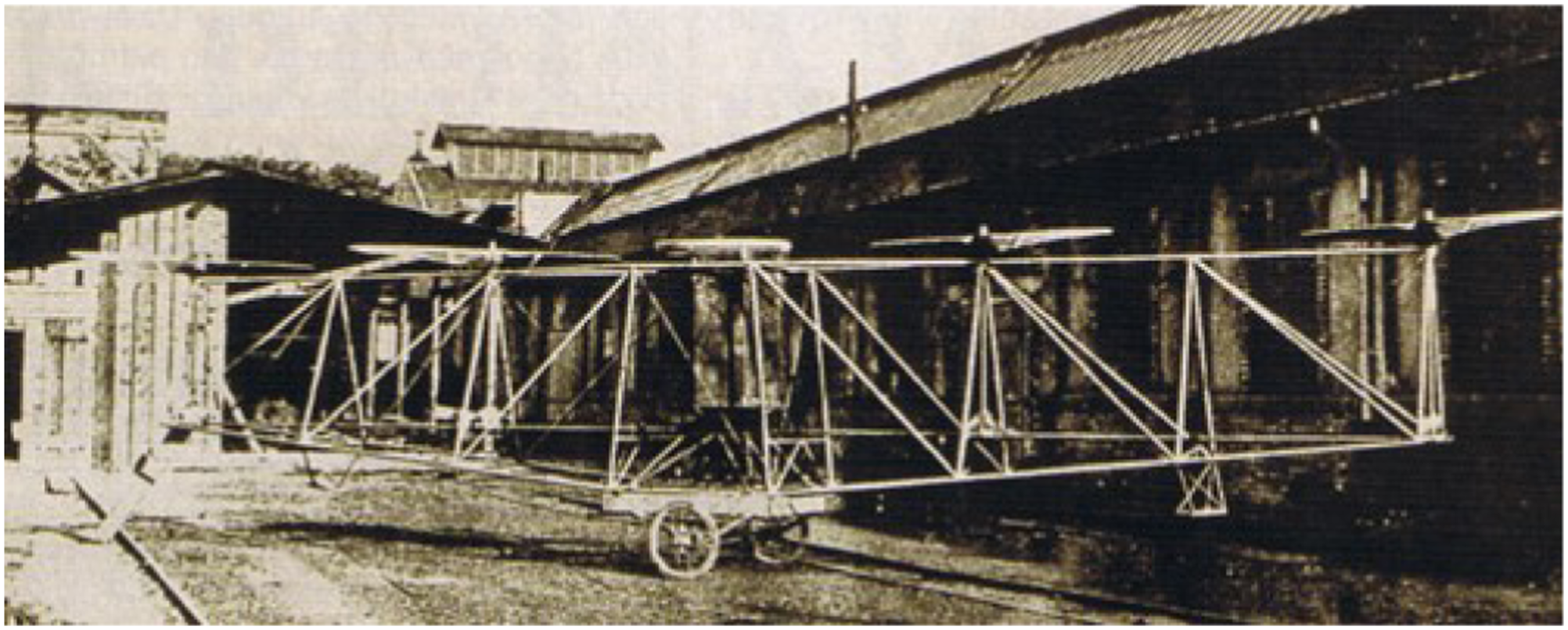
The first heavier-than-air electric aircraft appears to be the Petróczy-Kármán-Žurovec number 1 (PKZ-1),7,8 a static tethered observation platform that was designed to carry an observer and his equipment to the desired height. The design by Major Stephan Petróczy, Dr. Ing. Theodor von Kármán, and Ensign Vilém Žurovec avoided the problem of battery weight by using a ground based electric generator, and multiple tethers for stability. The PKZ-1 (shown in Figure 1) consisted of a lattice structure, welded from steel tubes, creating a beam of triangular cross-section. An electric motor was placed in the middle of the beam and a gondola for observers was built above it. The electric motor with an expected output of 250 hp (but actual output 190 hp) was supplied by Austro-Daimler. Four test flights of the PKZ-1 took place in March 1918 at the airship base in Fischamend. On the second attempt, there were three men in the gondola and PKZ-1 ascended to a height of half a meter, which was the limit of the tethers for that test. Unfortunately, the aluminum motor winding burned up on the fourth attempt and the PKZ-1 was not repaired. The PKZ-1 tethered platform.
7
The development of free flying electric aircraft would require substantial technical progress in electric motors and battery technology. In 1973, 55 years after the PKZ-1, aircraft manufacturer Heinrich Brditschka and an engineer with the Graupner model-building company, Fred Militky, enlisted the collaboration of Bosch (propulsion motor) and Varta (nickel-cadmium battery technology) to study the feasibility of an all-electric aircraft.9–11 They converted an HB-3A motor glider into the first electric manned airplane: the MB-E1 (Militky-Brditschka Elektroflieger No. 1), shown in Figure 2. On 21 October 1973, the MB-E1 took to the skies in Wels, Austria with Heinrich’s son, Heino Brditschka, at the controls. The maiden flight lasted for about 9 min and achieved an altitude of 300 m.
10
However, further advancement in battery and motor technology would be required to achieve practical electric flight. Militky Brditschka MB-E1 - the first manned aircraft powered solely by batteries.
9
First flight on Octobrer 21, 1973.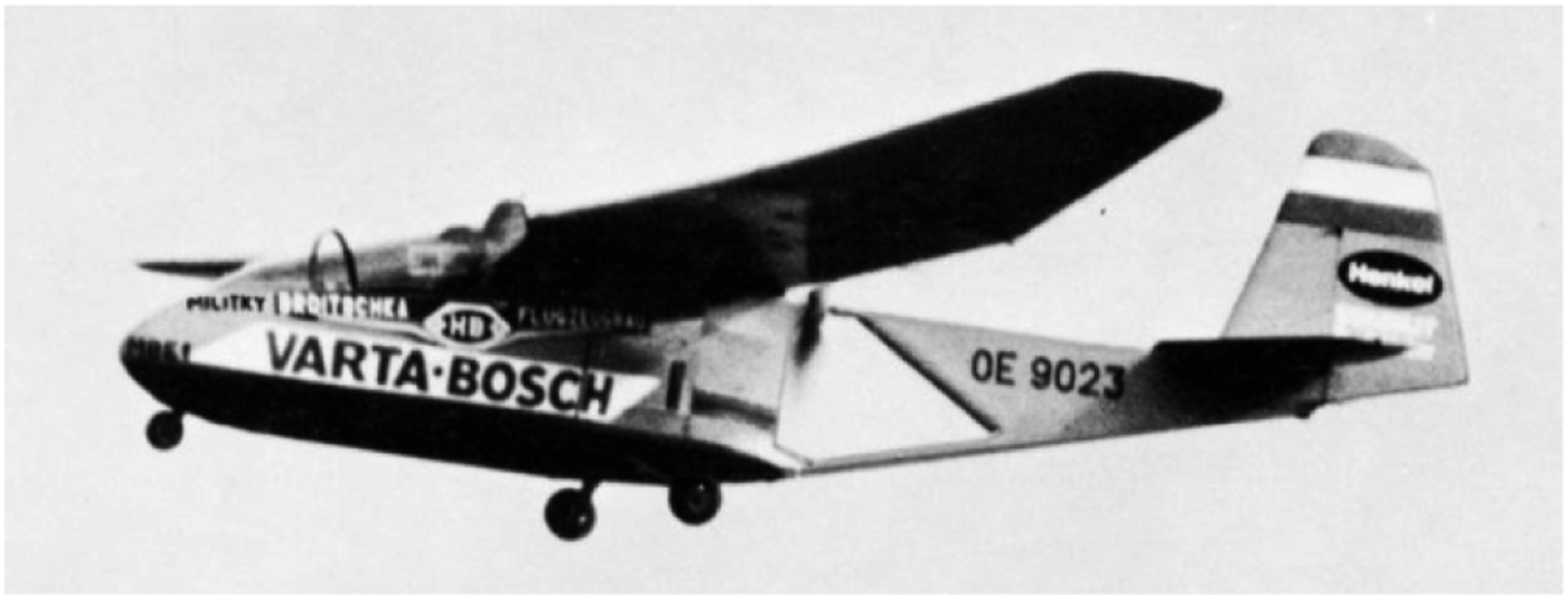
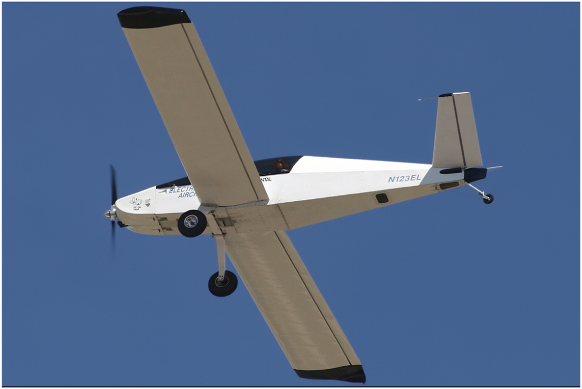
Thirty five years later, in 2008, battery and motor technology had improved substantially—leading to the debut of the ElectraFlyer-C at the Experimental Aircraft Association AirVenture in Oshkosh
12
(Figure 3). This all-electric, single passenger aircraft, fitted with a custom built lithium polymer battery pack was able to cruise at 70 mile/h for 1–1/2 to 2 h and charged in as little as 2 hours. The Electric Aircraft Corporation Web site states that the “ElectraFlyer-C was the first real electric airplane in the world. It was designed and built as a prototype and proof of concept for economical electric flight.”
13
Interestingly, the reports of the event comment on how the ElectraFlyer-C “wowed the crowd with its quietness,”
12
highlighting the opportunity for electric aircraft to be quiet. ElectraFlyer-C flown at Oshkosh AirVenture, August 2008.
12
Preparation for an eVTOL revolution: 2010–2016
At the beginning of the second decade of the 21st century, things were quietly coming into place for an eVTOL revolution. This subsection will discuss some of the key prototypes and demonstrators that were proving the feasibility of electric VTOL aircraft. The next subsection will deal with the explosion of eVTOL aircraft designs and flying aircraft that started in the latter half of the decade.
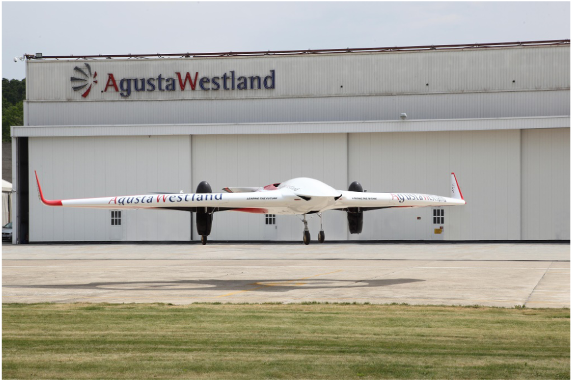
The first eVTOL technology demonstrator was the Augusta Westland Project Zero hybrid tiltrotor/lift fan aircraft. It was developed to investigate the use of all electric propulsion and other advanced technologies in a vertical lift aircraft. Project Zero was approved in December 2010 and by June 2011, a full-scale demonstrator (see Figure 4) performed an initial tethered flight at Cascina Costa, Italy.14–16 The Project Zero demonstrator was not flown in forward flight. Augusta Westland Project Zero aircraft in hover. The first tethered flight was in June 2011.
14
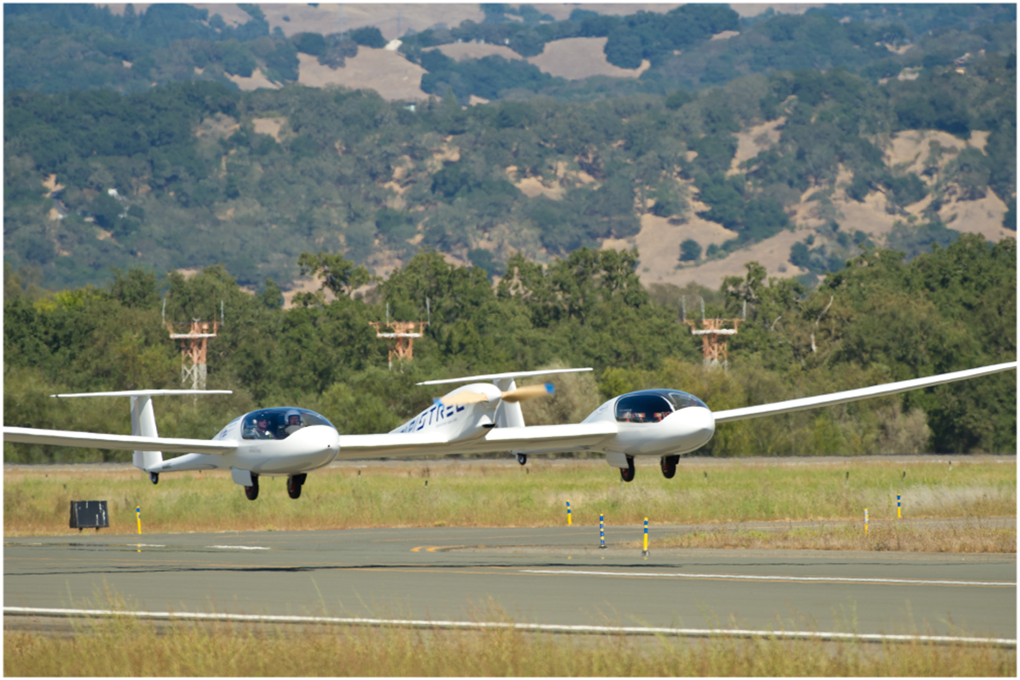
A short time later, in late September 2011, Google sponsored the CAFE Green Flight Challenge at the Sonoma County Airport in Santa Rosa, California. Three aircraft competed and two met the challenge requirements to fly 200 miles in less than 2 h and use less than the energy equivalent of one gallon of fuel per passenger. The first place prize of $1.35 M was won by the Pipistrel-USA.com team led by Jack Langelaan of State College, Pennsylvania.
17
Pipistrel’s new, twin-fuselage plane (shown in Figure 5) was created by combining two Taurus G2 fuselages, connected by a 5-m-long spar. A 145-kW brushless electric motor, developed for Pipistrel’s new 4-seat Panthera aircraft, is mounted between the passenger pods and drives a 2-m-diameter, two-bladed propeller in a tractor configuration. The Taurus G4’s full wingspan is about 21.36 m (75 feet) and it flew 200 miles nonstop while achieving 403.5 passenger mpg.18,19 This was a significant demonstration that efficient electric aircraft were indeed “coming of age.” Pipistrel Taurus G4 at the CAFE/NASA green flight challenge, September 2011.
20
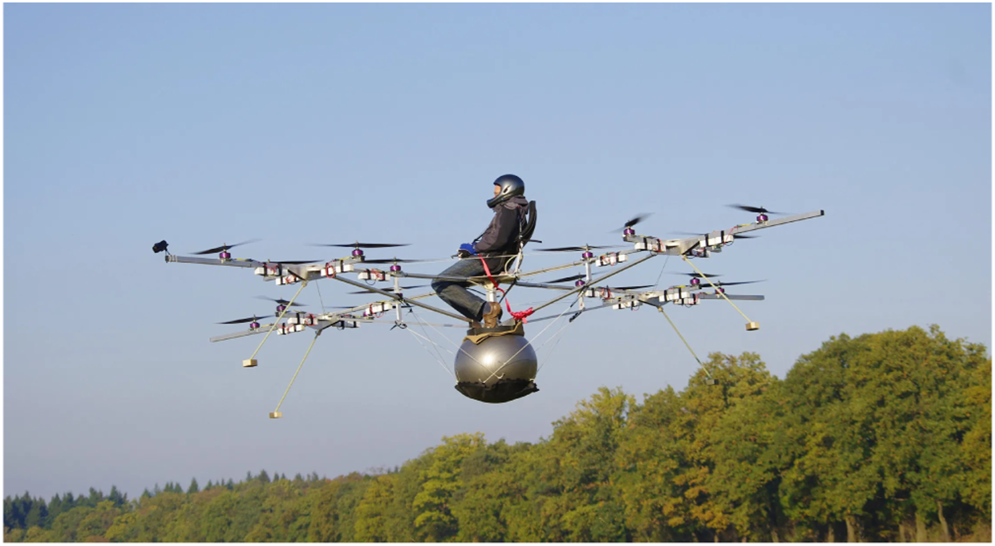
Soon after, the Volocopter VC1 (shown in Figure 6) would conduct the first manned flight of an electric multicopter according to the Guinness Book of World Records. The VC1 was flown by Volocopter co-founder, primary designer, inventor and builder, Thomas Senkel on 21 October 2011.
21
Next, Zee Aero (now Wisk), originally under the leadership of Professor Ilan Kroo of Stanford University, developed a proof of concept vehicle with a series of high, vertically-mounted mounted electric propellers (See Figure 7). The proof of concept made its first unmanned hover in Dec. 2011, and in Feb. 2014, completed its first transition from hover to forward flight.
22
Volocopter VC1 - first manned flight of a multicopter, 21 October 2011.
21
Zee Aero proof of concept aircraft: first hover, December 2011; first transition February 2014.
22
Although not known at the time, both Volocopter and Zee Aero were learning how to develop an eVTOL that could be commercially successful. In fact, 17 November 2013 was the first flight of the new two-seat Volocopter VC200 aircraft (see Figure 8). The VC200 was able to hover indoors and by February 2014 the VC200 transitioned to forward flight.
23
Contemporaneously, the first consumer drone (the DJI Phantom I) became commercially available in January of 2013. Many other companies were secretly developing their eVTOL aircraft as well. It is now known that in 2015 Joby was testing a subscale prototype
25
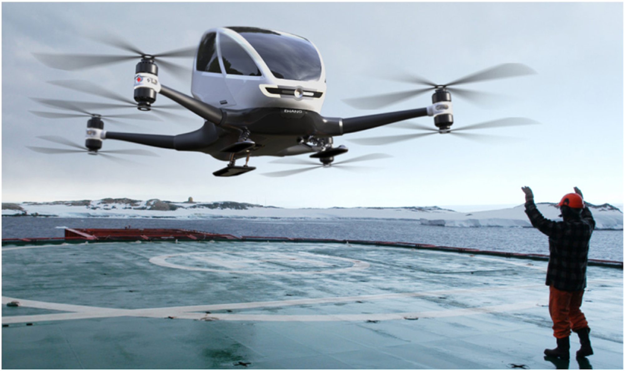
and EHang was flying their EHang 184
26
(1-passenger, eight propeller, 4 arm) aircraft (see Figure 9). Volocopter VC200, hover 17 November 2013; transition February 2014. (Photo credit Ref. 24). EHang 184 announced 6 January 2016 at CES. (Photo credit Ref. 28).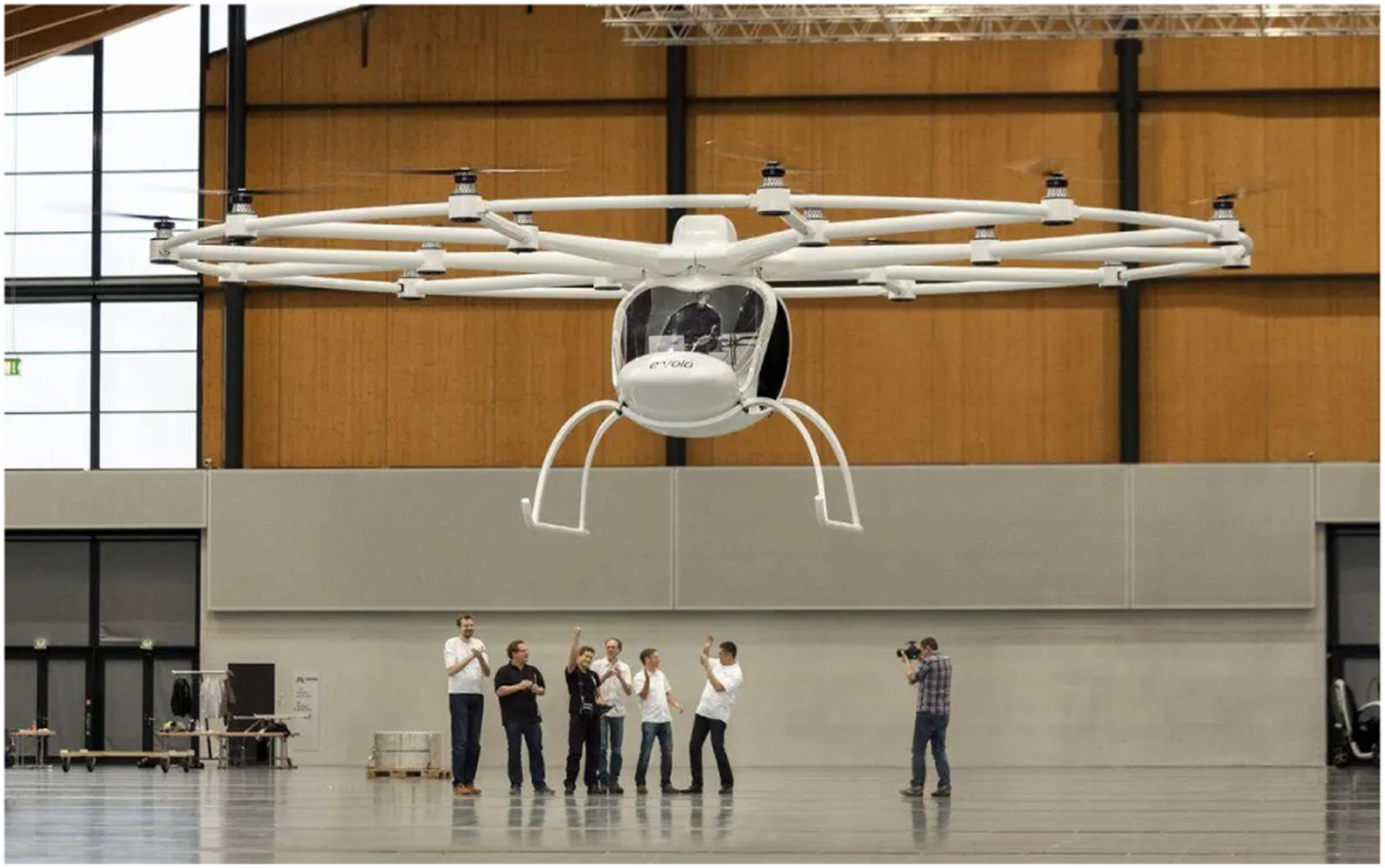
The final piece for the revolution to “come out of the dark” happened on 1 October 2016 when Uber released the landmark Uber Elevate white paper: “Fast-Forwarding to a Future of On-Demand Urban Air Transportation.” 27 This paper put into focus the key issues that needed to be addressed for eVTOL aircraft to be successful and Uber took the lead in defining objective targets for range, noise levels, infrastructure, etc. It gave the manufacturers targets and a significant potential customer.
An Explosion of new eVTOL vehicles: 2017–2021
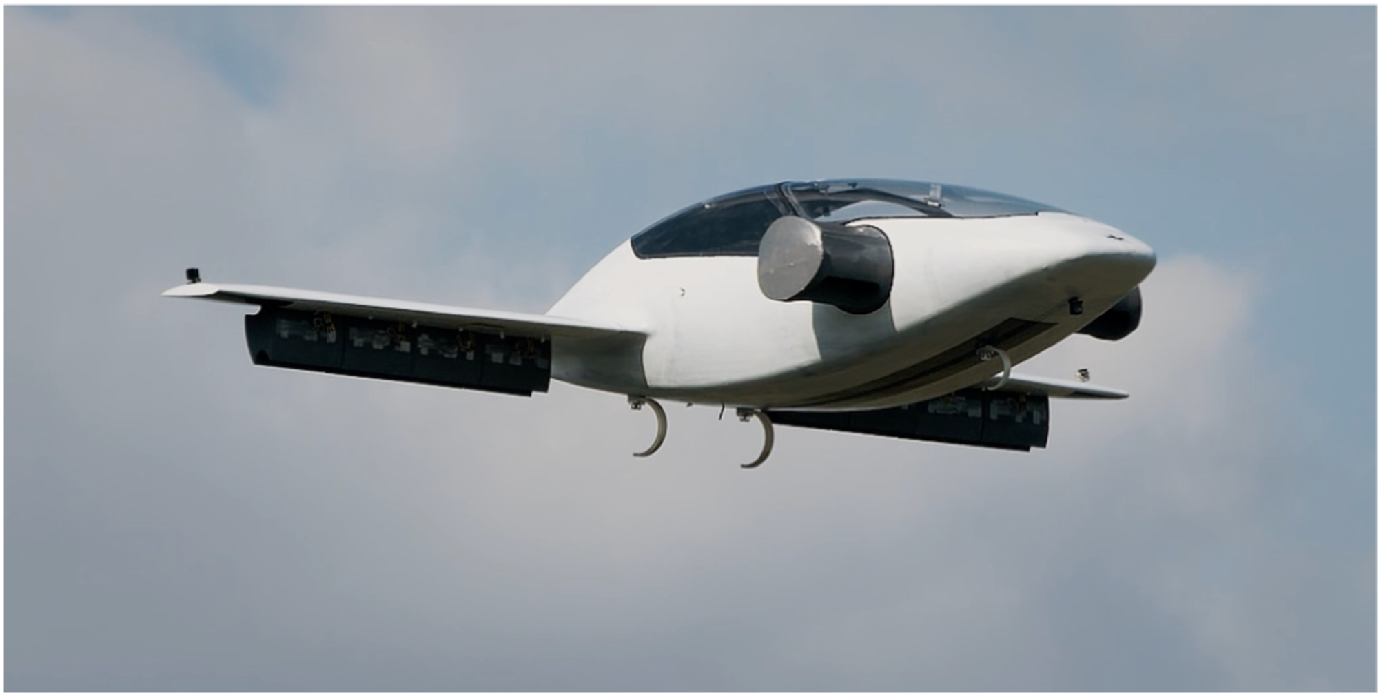
In the later part of the decade, many previously secret projects were revealed to the public. In April 2017, Lilium GmbH, a Germany-based start-up founded in 2015, flew the first flight of the Eagle prototype aircraft.
29
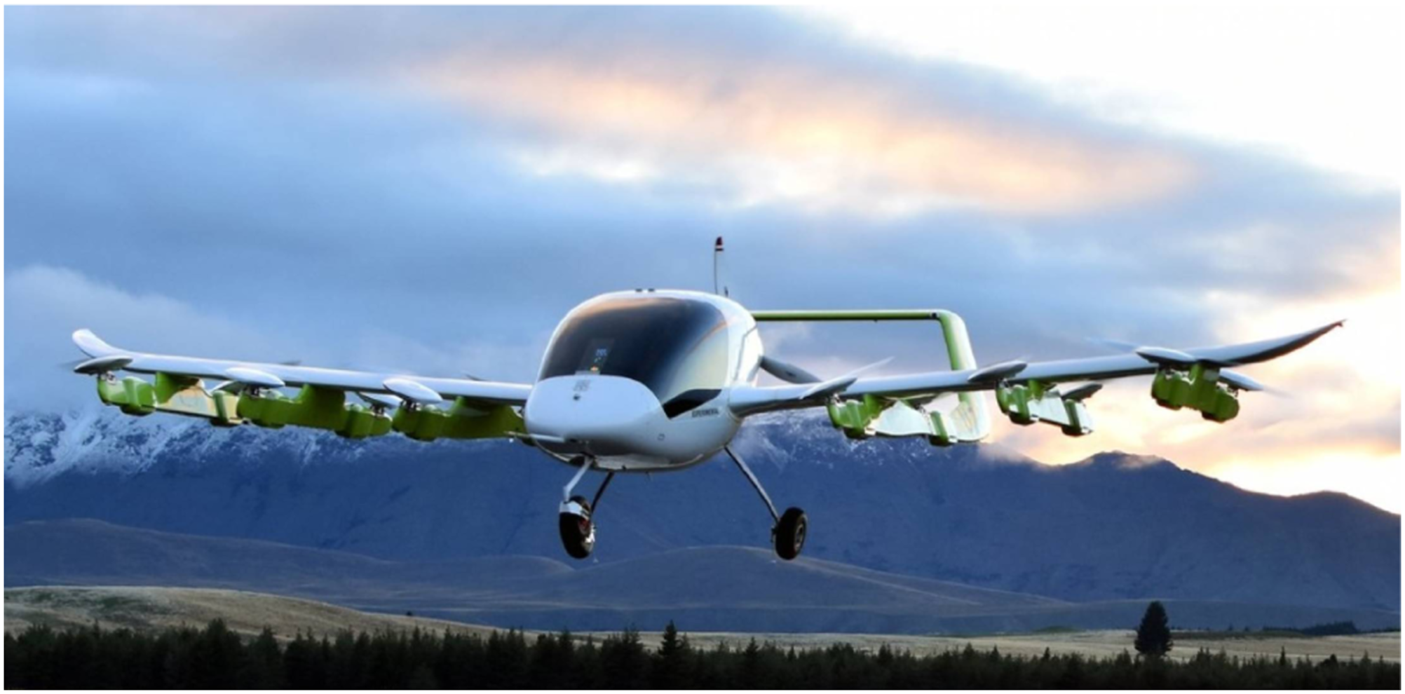
This aircraft, shown in Figure 10, was unique in that it used 36 powered fans (12 in each wing and 6 in each forward canard) for lift and propulsion. Kitty Hawk also started flight testing of the Cora aircraft
30
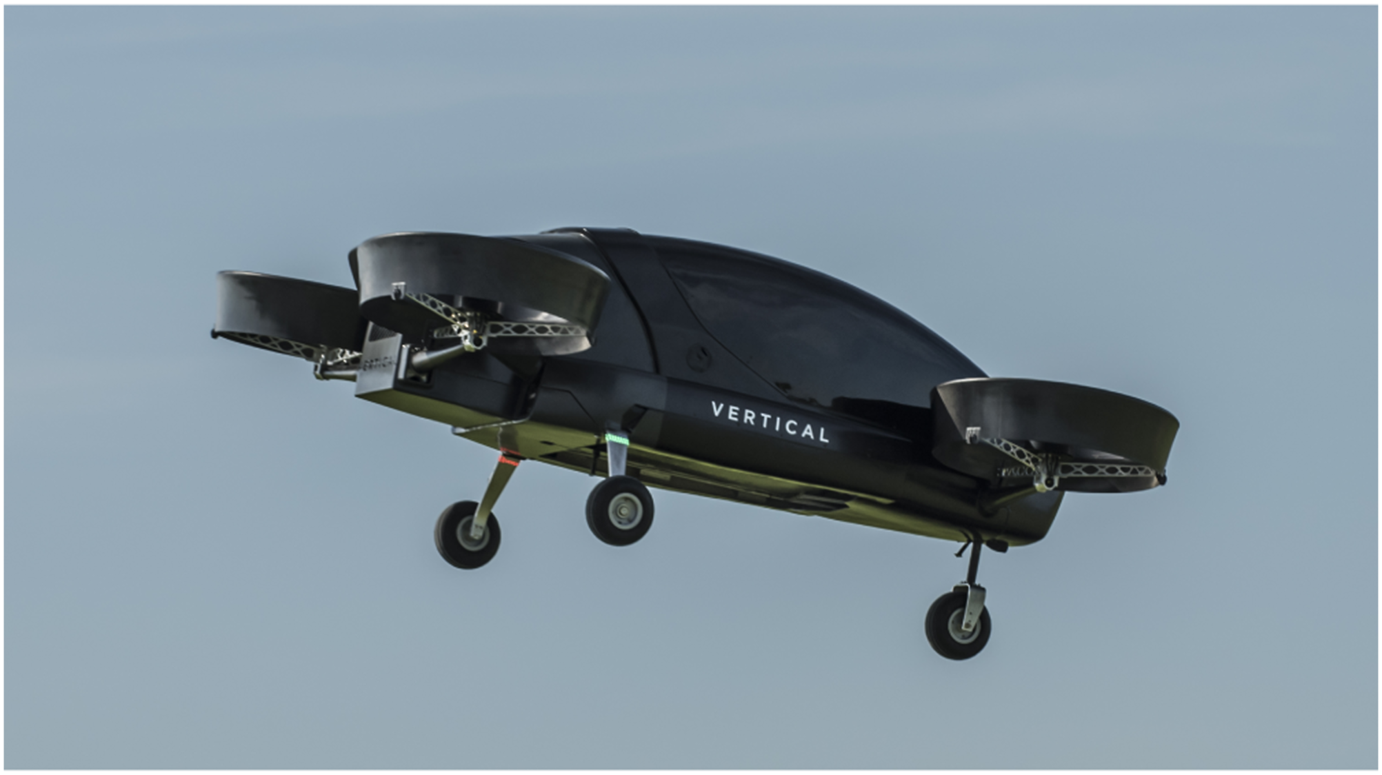
(see Figure 11) in California and New Zealand. The Cora is a two-seat autonomous aircraft with 12 lift propellers and a pusher prop. On 25 August 2017, Vertical Aerospace
31
flew the VA-X1 demonstrator (Figure 12) indoors for its first flight. The VA-X1 demonstrator used 4 shrouded 3-bladed propellers for lift and propulsion. Lilium Eagle prototype, first flight April 2017. (Photo credit Ref. 32). Kitty Hawk Cora, flight testing in 2017. (Photo credit Ref. 33). Vertical Aerospace VA-X1, first flight 25 August 2017.
31
In 2018, several more manufacturers demonstrated their technology through first flights. On 31 January 2018, Airbus A3 Vahana
34
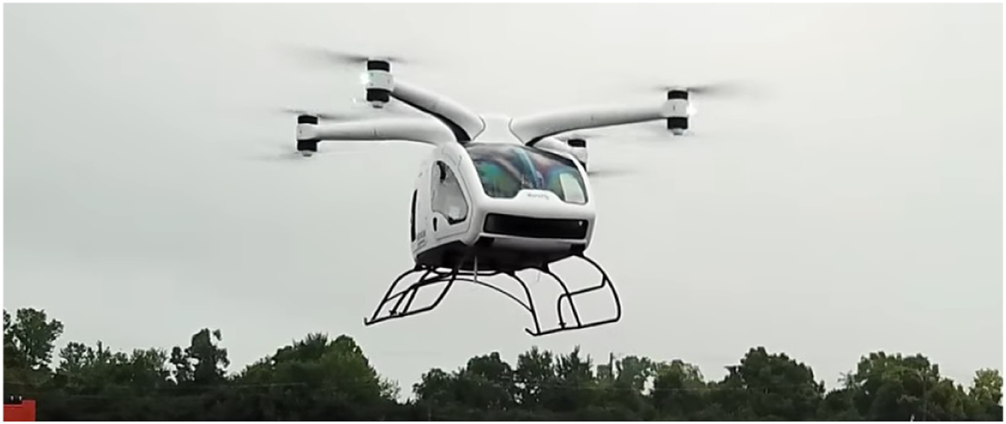
(Figure 13) flew its first flight. This aircraft has eight propellers mounted on two tilting wings. On 30 April 2018 the Moog Surefly
35
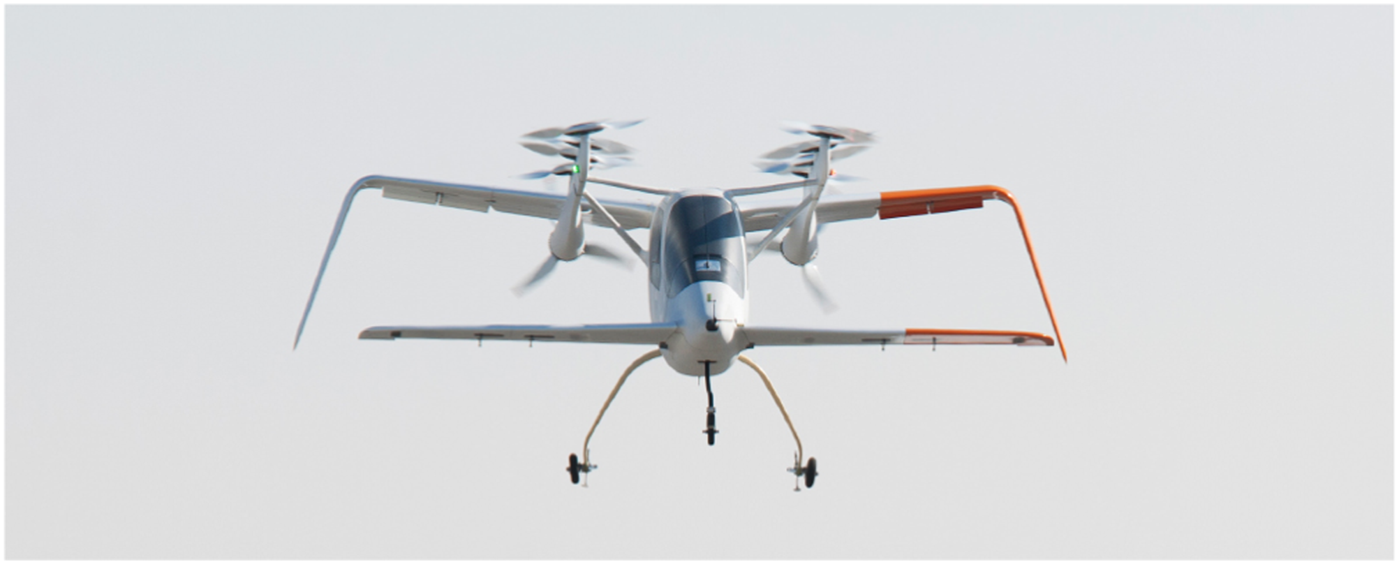
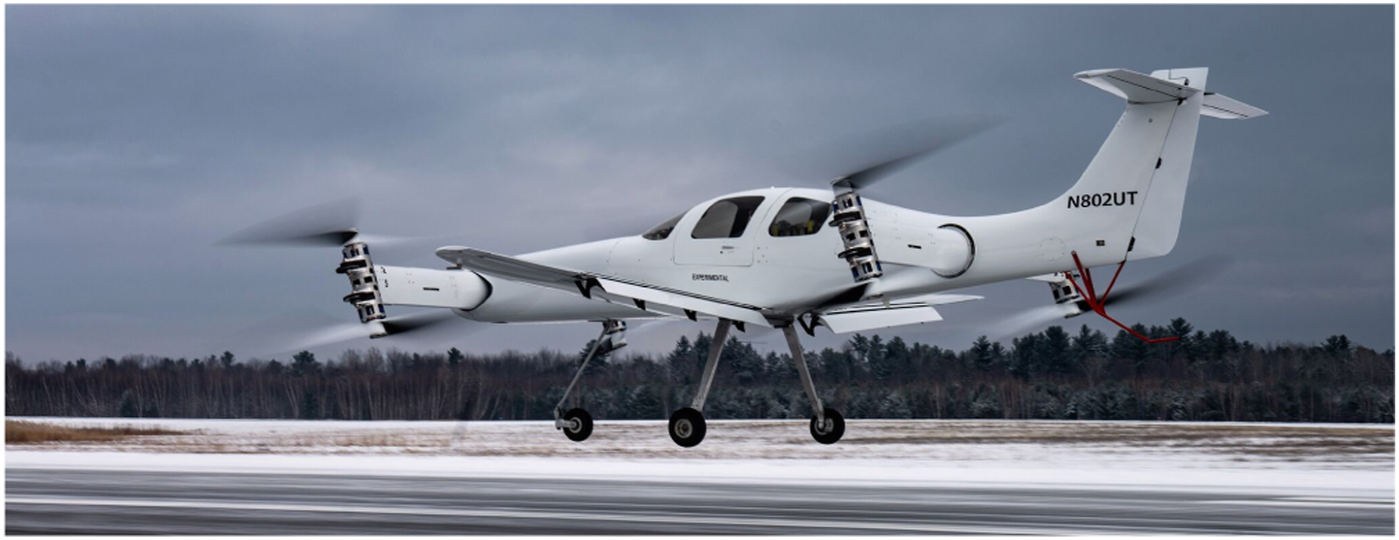
(Figure 14) flew its first flight. The configuration of the Surefly is somewhat similar to the EHang 184, but the 4 arms with the counterrotating propellers are mounted above the aircraft instead of close to the ground. Beta Technologies flew their Ava XC technology demonstrator
36
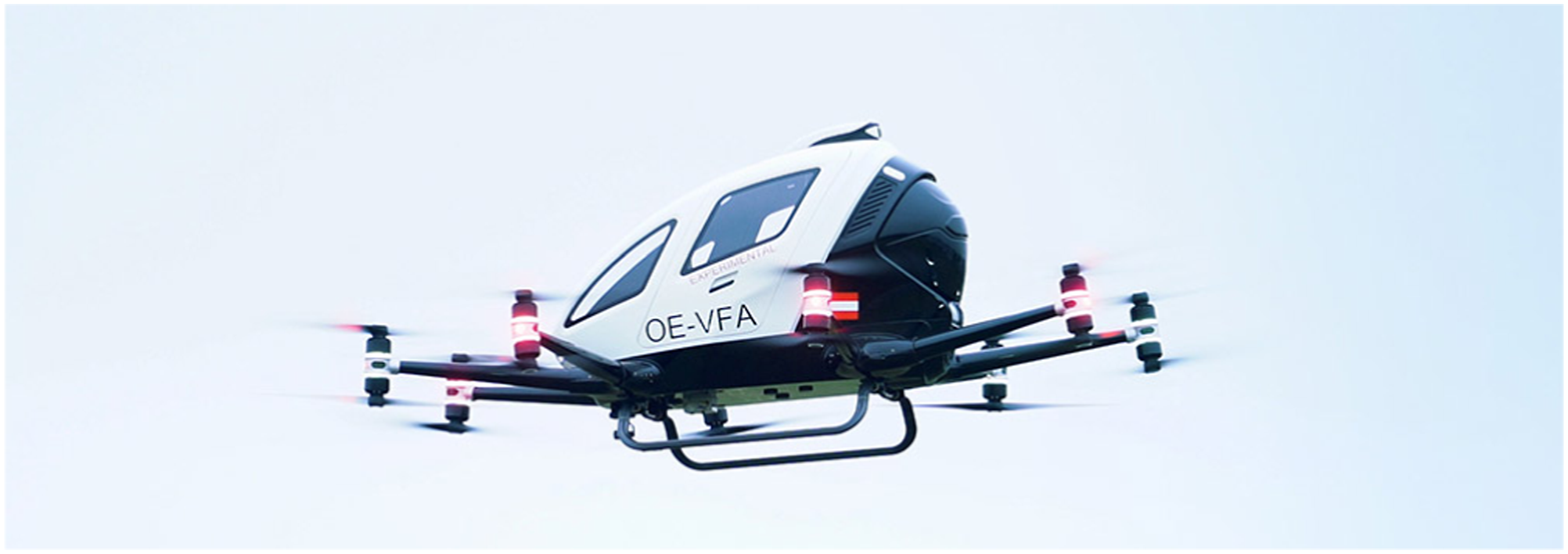
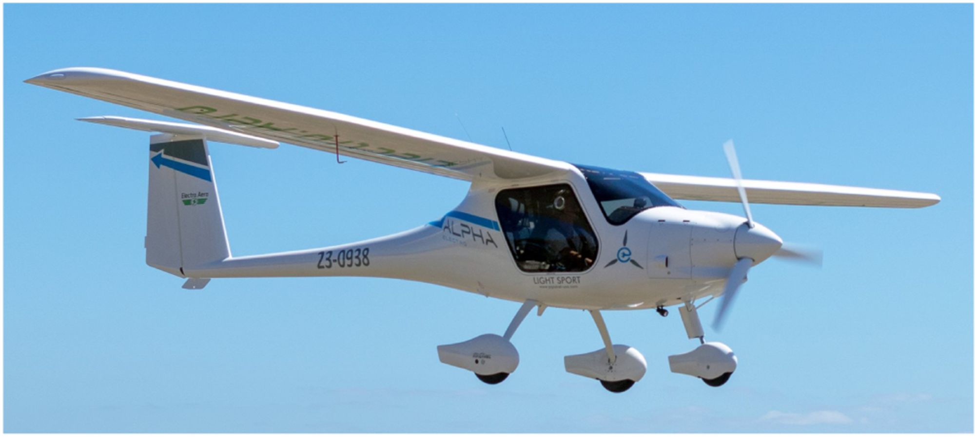
on 22 June 2018 (Figure 15) with 4 contrarotating, tilting rotors mounted on the wing tips of a vehicle that resembles a fixed wing aircraft. As with demonstrators developed by other manufacturers, the Ava XC was developed to gain familiarity with eVTOL technology. Also during 2018, EHang was testing its 216, a two-passenger aircraft with 16 propellers mounted on 8 arms (Figure 16). By July 2018 the EHang 216 had flown over 1000 manned flights.37,38 For comparison with the fixed-wing electric aircraft world, at the end of 2017 the Pipistrel Alpha Electro trainer (Figure 17) was officially released to customers with significant success.
39
This aircraft has an endurance of 1 h plus a 30 min reserve, short take-off distance, and 1000+ fpm climb. The Alpha Electro is also designed to recover 13% of the energy upon each approach.
40
Airbus A3 Vahana, 1/31/2018. (Photo credit Ref. 41). Beta Technologies Ava XC technology demonstrator, first manned free flight 22 June 2018.
36
Pipistrel Alpha Electro, world’s first 2-seat electric traine. (Photo credit Ref. 44).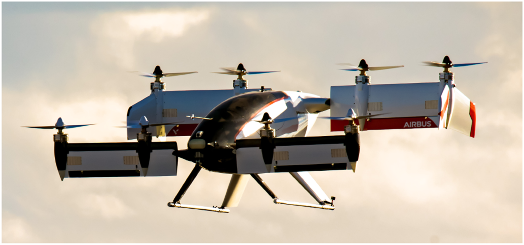
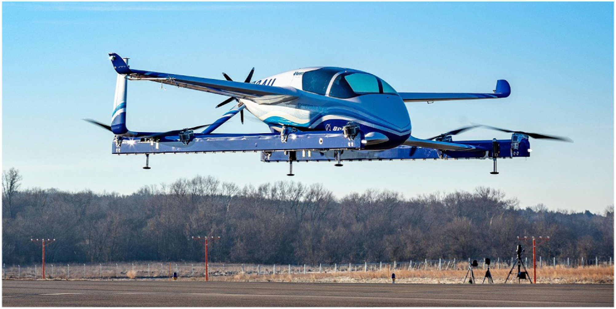
The public presentation of vehicles continued in 2019, starting in January when Aurora Flight Sciences, an independent subsidiary of Boeing, hovered a full-size prototype of their Pegasus Passenger Air Vehicle (PAV) on 22 January 2019 at the Manassas Regional Airport in Manassas, Virginia (Figure 18). Just a few months later on 4 June 2019, the Pegasus PAV crash-landed when the autoland function inadvertently entered ground mode and commanded the motors to shut down.
45
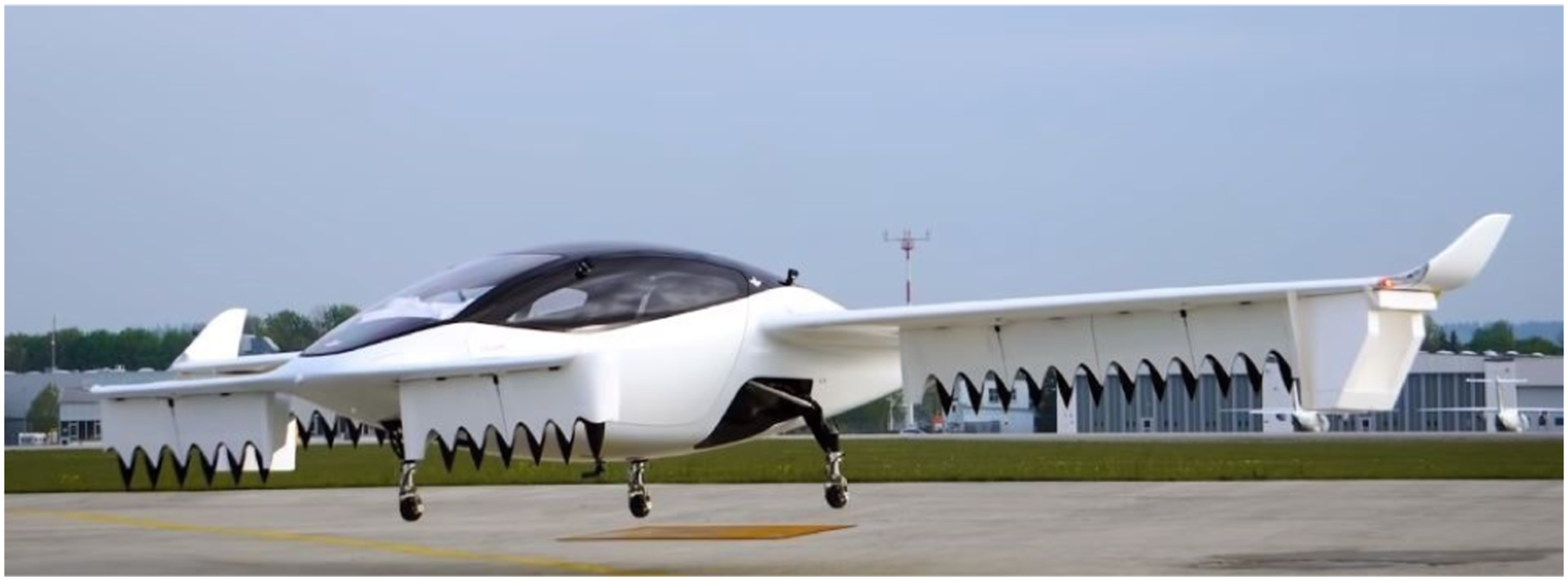
On 4 May 2019, Lilium flew its first flight of an untethered and unmanned five seat Lilium Jet at the Special Airport Oberpfaffenhofen in Munich, Germany (Figure 19). The full-scale prototype was powered by 36 electric ducted fans in configuration inspired by the Eagle prototype aircraft. After the first flight, which consisted primarily of hover, the Lilium Jet has expanded its flight envelope to include conversion to forward flight using the wing for lift, and several safety tests.
46
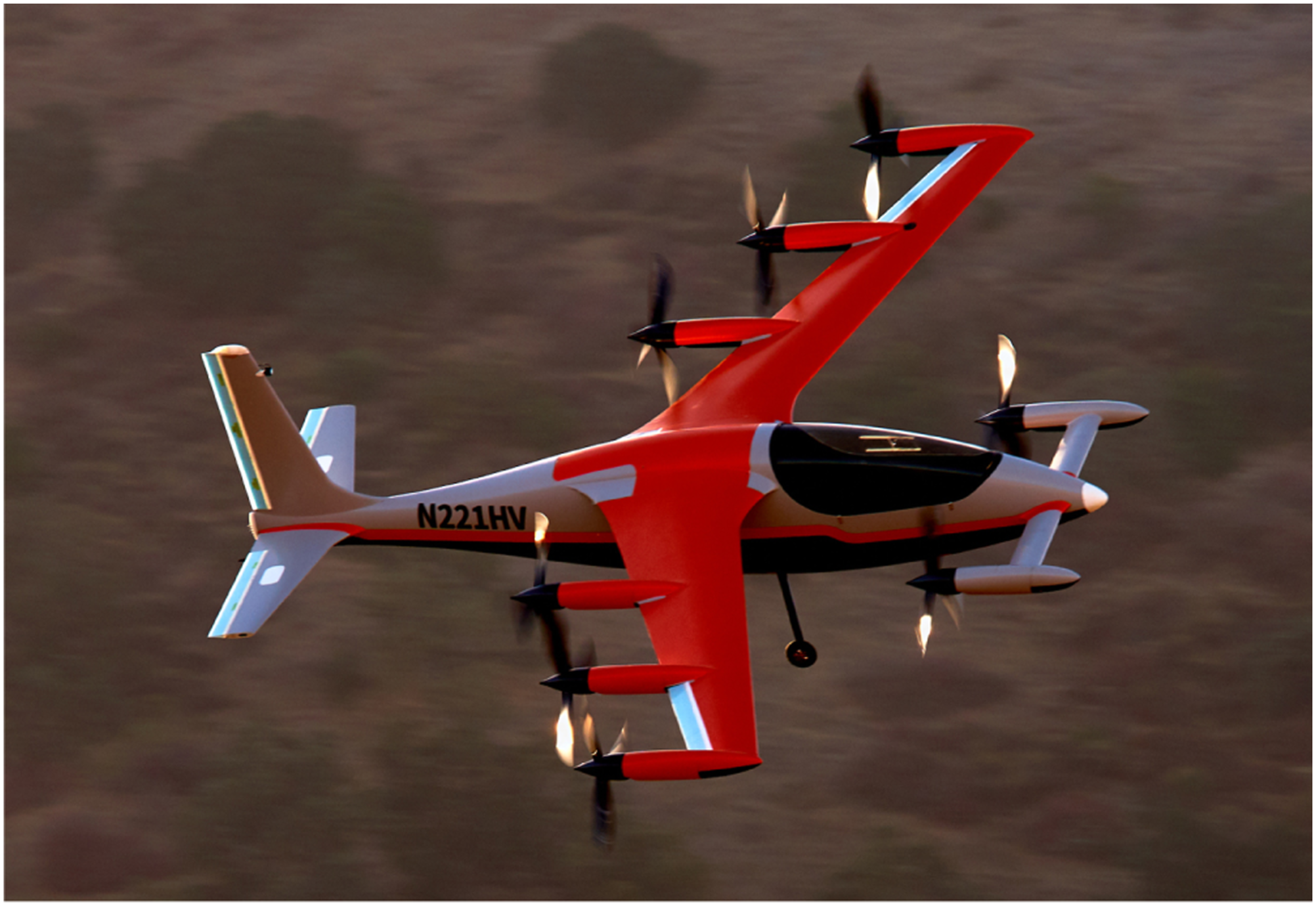
Then on 3 October 2019, Kitty Hawk revealed that they had been secretly developing a single seat electric aircraft known as the Heaviside (Figure 20).47,48 The Heaviside features a front wing with two propellers, six propellers on the main forward swept wing, and a fairly conventional empennage. The propellers are all behind the wings and tilt downward for vertical flight. Later in October 2019, a software timing error lead to a crash of the Heaviside during flight testing.
49
The advances and setbacks show the challenges that are part of developing a new type of air vehicle. Aurora Flight Sciences (Boeing) Pegasus PAV, first flight 22 January 2019.
45
Lilium Jet 5-seat prototype, first untethered flight 4 May 2019.
46
Kitty Hawk Heaviside, revealed 3 October 2019.
47
Joby Aviation announced their S4, four passenger eVTOL aircraft (Figure 21) in January 2020.
50
Quoting Ref. 50: “Joby Aviation’s S4 air taxi 2.0 is a five seat eVTOL (one pilot and four passengers) vectored-thrust aircraft using six tilting propellers which are located on both the fixed wing and its V-tail. Four propellers tilt vertically including its entire motor nacelle, and two of the propellers tilt vertically with a linkage mechanism. The aircraft has a very modern and futuristic design with large windows for spectacular views and has a tricycle-type retractable wheeled landing gear. The company reports their aircraft is 100 times quieter than a helicopter during takeoff and landing with a near-silent flyover.”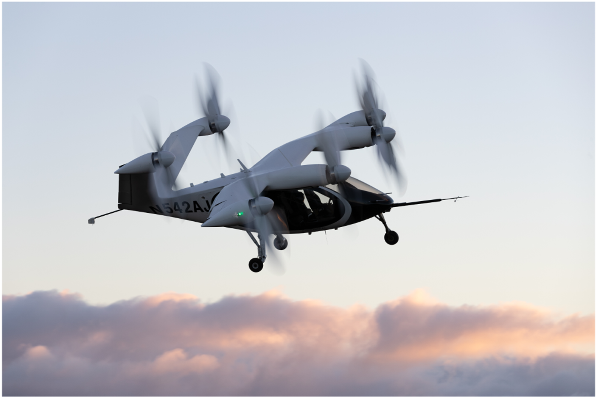
Throughout 2020, more information about the Joby S4 became available, including information about a piloted test flight in early 2017, plans for a manufacturing plant in Marina, California, and by the end of 2020 Joby received the first airworthiness approval from U.S. Air Force for electric VTOL aircraft. 51 By mid 2021, Beta Technologies Alia, 52 Lift Aircraft Hexa, 53 and Kitty Hawk Heaviside 54 had also received U.S. Air Force airworthiness approvals.
This review of eVTOL vehicles, especially in the last 5 years, highlights the wide range of eVTOL vehicles currently under development and in flight testing. This wide variety of configurations has been enabled by distributed electric propulsion. The unique features of electric aircraft enabled by this new technology are described in the next section.
Unique features of electric aircraft
As the preceding review of electrical aircraft illustrates, a wide range of electric aircraft are being developed, most having configurations that depart significantly from those of conventional airplanes and helicopters. While it is difficult to generalize across such a wide variety of concepts, there are a few common characteristics of these vehicles which offer new challenges for the aeroacoustician, but also present new opportunities for the reduction of noise. Although these aircraft use quiet electric motors instead of noisier combustion engines, this is not likely to have a significant effect on the overall noise radiation of the vehicle, because the noise of rotor and propeller driven aircraft is generally dominated by the aerodynamically-generated noise of the rotating blades. Instead, the main acoustic impacts of electrification are a result of the new freedoms of electric propulsion, especially distributed electric propulsion, offered to the aircraft designer.
Distributed electric propulsion is enabled by the relatively low weight and complexity of electric motors and power delivery systems, which allows multiple rotors or propellers to be integrated across the aircraft. For example, lift+cruise configurations, such as the Kitty Hawk (now Wisk) Cora and the Beta Technologies Alia, use entirely separate lightweight propulsion systems for rotor-borne vertical flight than they use for wingborne cruise. Other configurations, such as the Joby S4 and A3 Vahana, tilt the rotors during the transition from vertical to forward flight, taking advantage of the reduced weight and complexity of electric propulsion systems to greatly simplify the mechanisms for tilting the rotor nacelles or wings. Unlike conventional helicopters, many eVTOL aircraft do not rely on rotors in edgewise flight to produce lift during cruise, considerably reducing the thrust required from the propulsion system during this stage of flight. Since the rotors are more lightly loaded during cruise, they can also be operated at lower tip speeds than during vertical flight. Electric motors are comparatively well suited to variable speed operation because they are capable of efficiently producing torque over a wider range of shaft speeds than turboshaft or piston-driven combustion engines. While tip speed reduction can be effective in reducing aerodynamically generated noise (up to a point, as will be illustrated in a later section), more torque is required to produce the same thrust at lower tip speeds. This has resulted in many eVTOL designers favoring a large number of smaller rotors operating at higher shaft speeds and lower torque over fewer slower turning large rotors. However, several manufacturers, such as Joby, have developed high specific torque (torque per unit weight) motors to allow larger rotors to be used to reduce disk loading and power requirements during vertical flight.
Although distributed electric propulsion has reduced the mechanical complexity of these aircraft, the same cannot be said about the aerodynamic complexity of these configurations. With many rotors, propellers, and fixed aerodynamic surfaces, there is a strong possibility of unsteady aerodynamic interactions between these components, which can lead to noise generation. These interactions will occur most strongly between closely-coupled components, such as a propeller installed behind a wing. Furthermore, such configurations may also allow for interactions between components and propellers or rotors that are far downstream. These interactions are not well understood due to the instability, breakdown, and turbulent nature of wakes at long ages. Moreover, as these vehicles transition between vertical and horizontal modes of flight, the individual components will pass through a wide range of operating conditions with the potential for a variety of different aerodynamic interactions to occur.
Many aircraft featuring distributed electric propulsion also use the distributed propulsion system as a primary means of control. The thrust of the individual rotors or propellers is varied to control the total forces and moments on the vehicle, which will change in order to effect a maneuver or to stabilize the vehicle in response to external disturbances. Depending on the mode of flight, additional actuators such as aerodynamic control surfaces may also be employed. These systems are inherently “fly-by-wire,” with some level of automation existing between the pilot or operator’s commands and the response of the vehicle. In most cases, these vehicles are highly over-actuated for redundancy. This means that the rotors or propellers could be operated in many different ways to achieve the same flight condition, with the possibility of influencing the aerodynamic performance and radiated noise.
Physics of rotor noise generation
Ffowcs Williams – Hawkings equation
In their 1969 paper, Ffowcs Williams and Hawkings
1
used the powerful technique of generalized function theory to develop the equation that has become associated with their names. The FW-H equation is an exact rearrangement of the continuity equation and the Navier–Stokes equations into the form of an inhomogeneous wave equation with two surface source terms (monopole and dipole) and a volume source term (quadrupole). The FW-H equation
1
is the most general form of the Lighthill acoustic analogy
55
and is appropriate for predicting the noise generated by the complex motion of rotors, propellers and maneuvering aircraft. In differential form, the FW-H equation is given by the following inhomogeneous wave equation
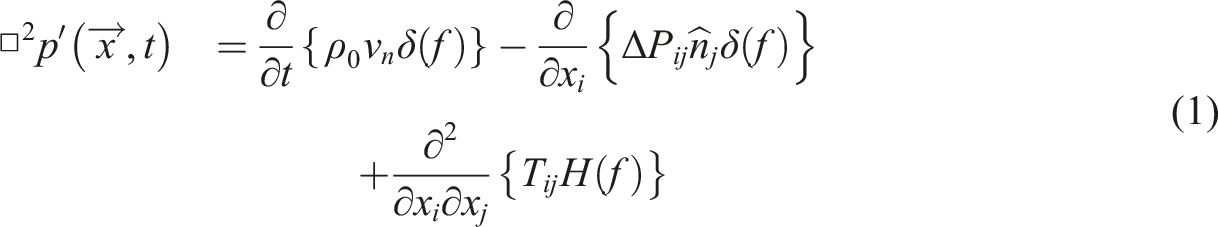
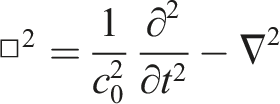
The FW-H equation is valid in the entire unbounded space; hence, a formal solution may be obtained by using the free-space Green’s function δ(g)/4πr, where
The quadrupole source term (a volume source) accounts for noise sources in the volume f > 0; i.e. outside of the surface f = 0.
The quadrupole term can also be seen as a correction to the propagation of the surface source (monopole and dipole) terms to account for deviations from the linear wave equation. For example, the quadrupole sources can describe nonlinear wave propagation and steepening; variations in the local sound speed; and noise generated by shocks, vorticity, and turbulence in the flowfield.
For example, at high subsonic, transonic, and supersonic tip speeds, rotors can generate an impulsive noise of high intensity due to the formation of local shocks in this volume. For edgewise rotors, such as helicopter main and tail rotors, the noise is known as high-speed-impulsive (HSI) noise, and has in-plane directivity in the direction of flight. Hence, the quadrupole source term is usually associated with HSI noise and is neglected for lower subsonic source speeds. The quadrupole source can also be used to model the broadband source terms associated with vorticity and turbulence in the flow, but in rotor and propeller noise prediction, alternative methods relating these sources to dipole (loading noise) sources have traditionally been used.
Shortly after the FW-H equation was developed, Farassat derived several integral representations of the solution to the FW-H equation—the most widely used formulation is known as Formulation 1A.
56
Farassat’s Formulation 1A neglects the quadrupole source, and may be written as follows

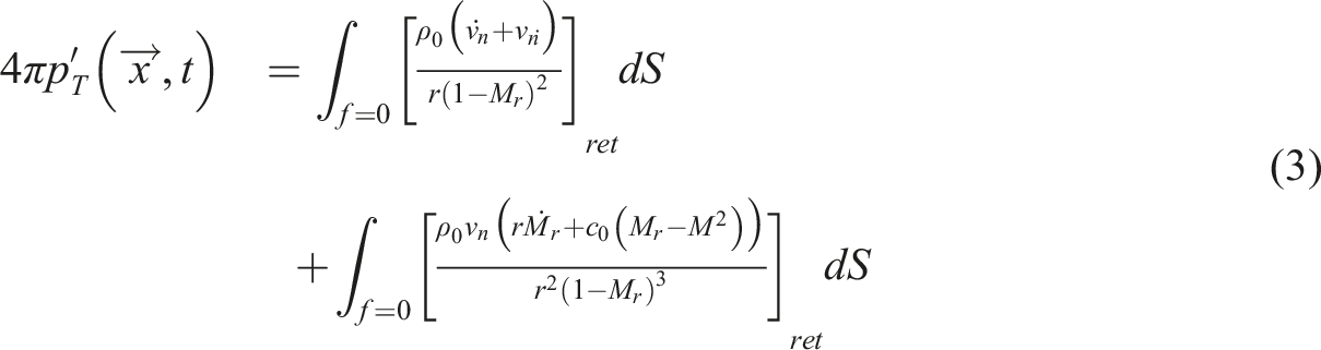
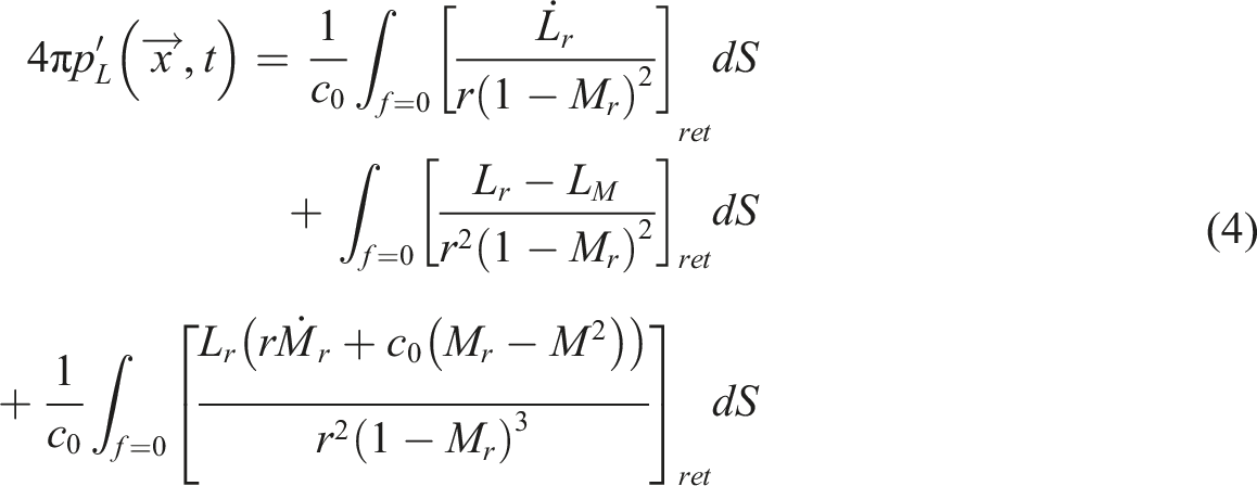
Examining equations (3) and (4), the terms with 1/r dependence are far-field terms since they decay according to acoustic spherical spreading; terms with 1/r2 dependence are near-field terms; and
All integrand terms are strongly affected by the Doppler amplification, but for an edgewise rotor, the speed of the vehicle and the blade motion combine to produce even higher values of M r when the blade is moving in the direction of flight. Thickness noise is strongly dependent on the tip-Mach number, and as such, tends to radiate most strongly in the plane of the rotor. Loading noise is also influenced by tip-Mach number, but to a lesser degree than thickness noise.
For rotors operating at lower tip-Mach numbers or even stationary surfaces, unsteady loading can be a significant source of loading noise. Notice that the first integral of equation (4),
Taxonomy of rotor noise sources
For rotating blades the three distinct noise sources described by the Ffowcs Williams and Hawkings (FW-H) equation—thickness, loading, and high-speed-impulsive (quadrupole) noise—may be present depending on the flight condition. Electric aircraft are expected to use lower tip speeds than helicopters to reduce noise; therefore, high-speed impulsive noise is not expected to occur, and thickness noise is unlikely to be as high as loading noise sources. Consequently, noise due to unsteady loading is likely to be the primary concern. Figure 22 shows a taxonomy of rotor noise sources, adapted from that Brooks and Schlinker,
57
to emphasize the loading noise sources expected to be important for electric aircraft. These sources are highlighted in blue. Taxonomy of rotor noise sources (adapted from Brooks and Schlinker).
57
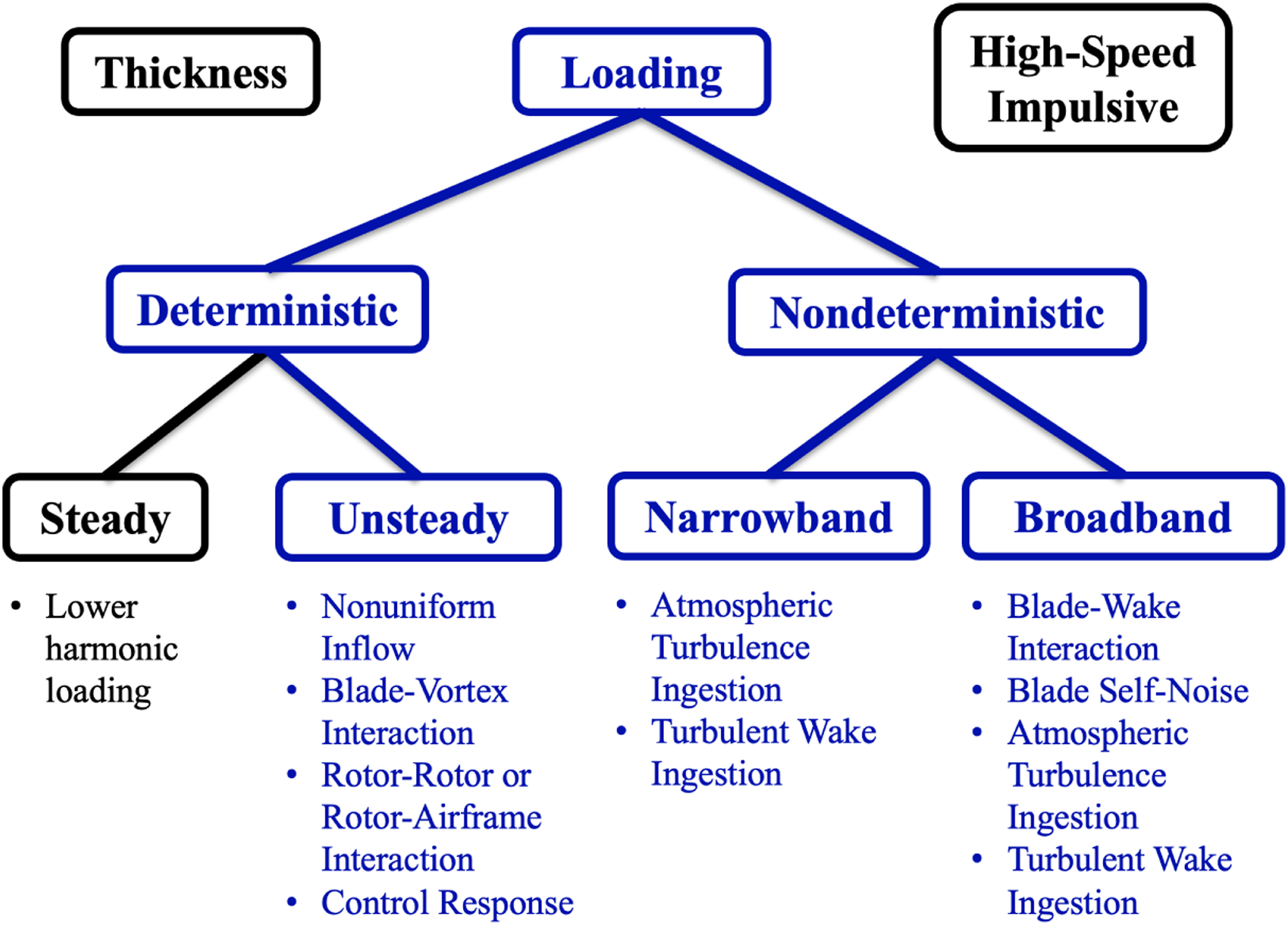
Loading noise can broadly be divided into deterministic and nondeterministic components. Furthermore, the deterministic loading is usually further subdivided as steady or unsteady, while the nondeterministic loading sources can be divided into narrowband and broadband noise sources. The steady, deterministic loading is due to lower harmonic loading and sometimes is referred as “loading noise”. Thickness noise and steady loading noise, when considered together, are also known as as rotational noise.
The unsteady deterministic loading noise is caused by a variety of unsteady loading sources, including nonuniform inflow, blade-vortex interaction, rotor-rotor or rotor-airframe interactions, and unsteady response to controls inputs. Nondeterministic narrowband loading noise (or narrowband random noise) is generally related to turbulence ingestion of atmospheric or a turbulent wake into the rotor or propeller. As the rotor “chops” several times through a turbulent eddy, the result is a narrowband random noise source, that is characterized as broad spectral peaks around the blade passage frequency and its harmonics. Broadband noise is characterized by a broad noise spectrum caused by unsteady turbulent loading due to blade-wake interaction, turbulence in the boundary layer (for blade self noise), and turbulence ingestion.
eVTOL rotor noise trends
The various noise sources for a notional eVTOL rotor are explored in this section to highlight the relative importance of the previously described rotor noise sources for eVTOL aircraft. Noise predictions are made using a tool called VSP2WOPWOP, which was developed for the preliminary assessment of eVTOL acoustic design trades. 58 VSP2WOPWOP is an open source tool that allows users to quickly generate rotor or propeller geometries using NASA’s OpenVSP 59 conceptual design software, analyze the aerodynamic performance using blade element methods, and then perform aeroacoustic analyses from the blade geometry and predicted airloads using PSU-WOPWOP.60–64 PSU-WOPWOP is a multifidelity aeroacoustic prediction code that solves Farassat’s Formulation 1A of the FW-H equation for arbitrary surface geometries and motions, making it well suited to the prediction of rotorcraft noise. 65 Semi-empirical broadband noise models are also included, in addition to a variety of signal processing functions and noise metrics. 66
Although the rotor geometry used here is notional, it has been developed to be representative of eVTOL aircraft. A top view of the geometry is shown in Figure 23. The rotor has a diameter of three m with a solidity of 0.2. Noise levels were predicted for a “hovering” operating condition with a fixed thrust of 2500 N. The observer is placed at a distance of 10 rotor radii from the rotor hub (i.e. 15 m) in the plane of the rotor. The tip Mach number was then varied across a wide range, from 0.3 (near stall) to 0.8, and the overall sound pressure levels (SPL) predicted using Formulation 1A for tonal noise and the Brooks, Pope, and Marcolini method
67
(described in more detail later) for broadband noise. The contributions of thickness, steady loading, and broadband noise—as well as the total SPL—are plotted against tip Mach number in Figure 24. Geometry of notional eVTOL rotor. Variation in noise by tip Mach number for notional eVTOL rotor.
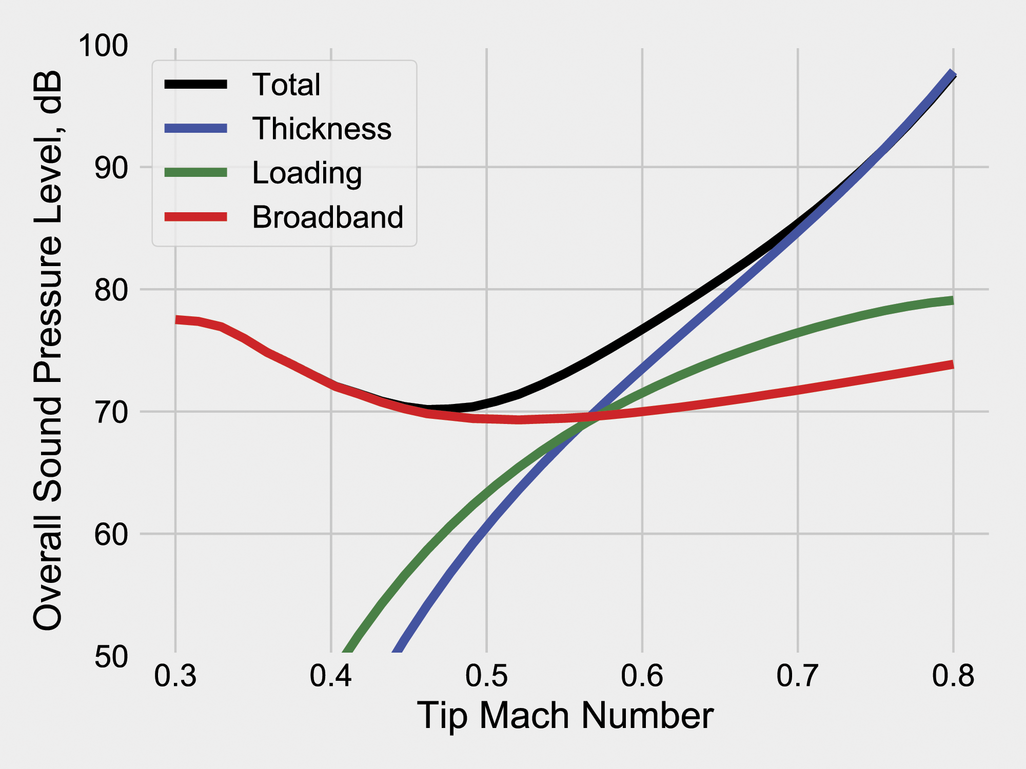
At high tip Mach numbers, thickness noise dominates the total noise levels. However, this source falls off quickly as the tip speed is reduced. Steady loading noise falls off less quickly, and becomes a significant contributor to the in-plane noise radiation at moderate tip speeds. The magnitude of both of these “steady” noise sources is primarily driven by convective amplification. In contrast, broadband noise is relatively insensitive to tip speed reductions. This is because the noise radiation is primarily driven by the unsteady surface pressure fluctuations, and not convective amplification. Similar trends should be expected for other forms of unsteady loading noise. Interestingly, the broadband noise levels begin to increase with decreasing tip speeds beginning at a tip Mach number of around 0.5. This is driven by an increase in turbulent boundary layer noise as the angle of attack of the blade sections increases, eventually leading to flow separation.
These results imply that there is likely to be an “optimal” tip speed for a given rotor geometry, below which additional tip speed reductions will be ineffective in reducing noise or will even increase it. At this “optimal” tip speed, the sources of unsteady loading—both deterministic and nondeterministic—will dominate. From interviews with leading eVTOL developers, 4 it appears that many rotors are already designed to operate near the “optimal” point for this notional rotor, at tip Mach numbers at or below 0.5. Lower tip speeds are likely achievable with low noise when the rotors are lightly loaded, such as during cruise. This suggests that mitigating the unsteady loading noise sources highlighted in blue in Figure 22 will be the primary concern of eVTOL developers seeking to develop low noise aircraft. Although little has been published on the noise of electric aircraft to date, insight can be gained from the existing literature regarding these noise sources for more conventional aircraft.
In the next section, the relationship between unsteady loading and the resulting the noise caused by aerodynamic interactions will be reviewed. This will be followed by a review of the literature on rotor broadband noise.
Noise caused by aerodynamic interactions
One likely source of unsteady loading noise for electric aircraft are aerodynamic interactions. For conventional rotorcraft—such as helicopters—aerodynamic interactions often occur between the rotor and its own wake, resulting in both deterministic (Blade–Vortex Interaction or BVI) and nondeterministic (Blade–Wake Interaction or BWI) noise. In addition to these noise sources, the complexity of electric aircraft configurations using distributed propulsion provides many opportunities for acoustically-significant aerodynamic interactions, such as interactions between two (or more) individual rotors or between the rotors and aerodynamic surfaces or other airframe components.
Blade–vortex interaction noise
Blade–Vortex Interaction (BVI) is the most significant source of noise associated with aerodynamic interaction for conventional rotorcraft, such as helicopters
68
and tiltrotor aircraft.
69
For these aircraft, BVI noise is generated by the interaction between the rotor and its own wake, which occurs most strongly during descending and maneuvering flight. As the rotor blades pass near the tip vortices formed by preceding blades, they experience a rapid fluctuation of aerodynamic loads.
70
This fluctuation results in the radiation of highly impulsive, and therefore annoying, noise. Figure 25 shows pulses typical of strong BVI extracted from one rotor revolution of measured data for a maneuvering Bell 206B helicopter. Blade–Vortex Interaction pulses from one rotor revolution of a Bell 206B helicopter (adapted from Ref. 71).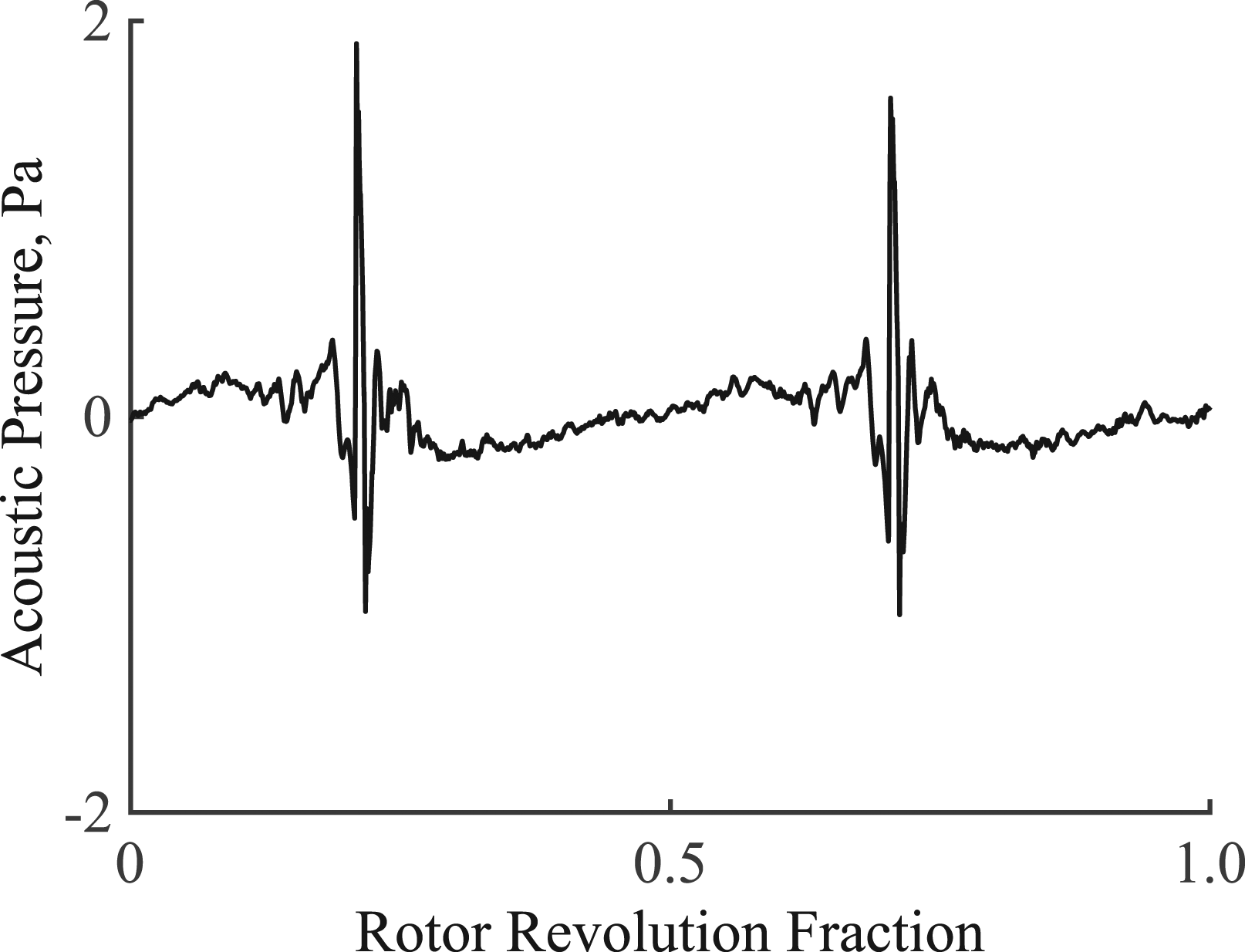
Since BVI noise is strongly dependent on the relative positions of the blades and the rotor wake, it is very sensitive to changes in the operating condition of the rotor. Figure 26 illustrates how the blades near the rear of the rotor disk interact with tip vortices previously formed at the leading edge of the rotor. The intensity and directivity of BVI noise is a function of the angle between the tip vortex and the azimuth angle of the blade during the interaction, which is determined by the top view geometry of the wake shown for an AS350 helicopter in Figure 26(a). The top view wake geometry is primarily determined by the rotation speed of the rotor and the true airspeed of the vehicle.
72
The intensity of BVI noise is also a strong function of the “miss-distance” between the rotor disk and the shed tip vortices. When the rotorcraft descends along a shallow trajectory, the wake will convect below the rear portion of the rotor disk, as shown in Figure 26(b), resulting in the onset of BVI noise. As the rotorcraft descends more steeply, Figure 26(c), the wake convects into the rotor disk, reducing the miss-distance, and increasing the intensity of BVI noise. Further increases in the rate of descent, shown in Figure 26(d), cause the wake to convect above the rotor disk, increasing miss-distance and reducing BVI noise from the peak level.
72
The wake geometry governing BVI noise.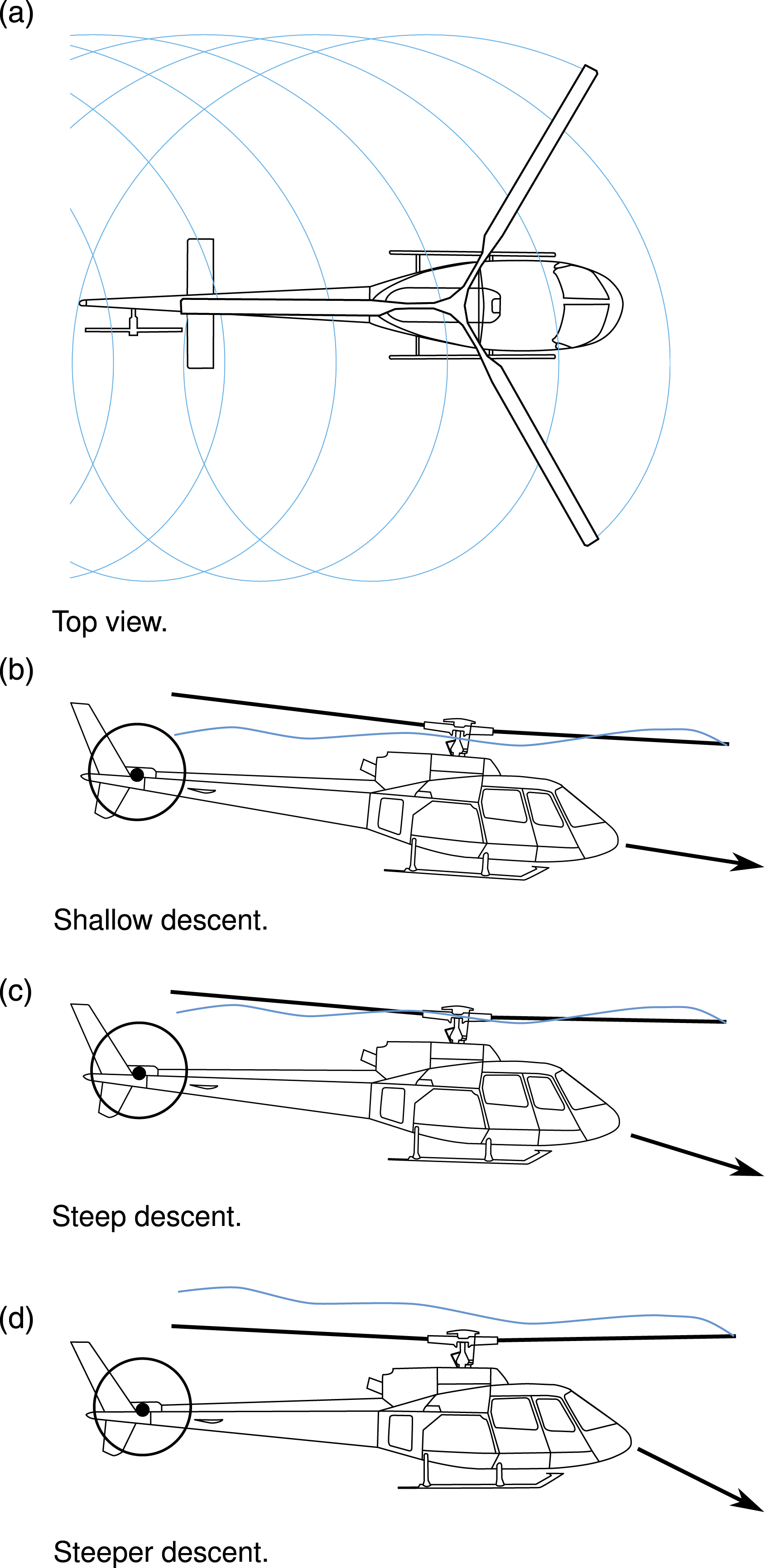
BVI is a significant source of noise for conventional rotorcraft, but can be effectively controlled through careful management of the vehicle’s operating state, as will be described later in this article. eVTOL aircraft will likely also experience BVI, both from rotors interacting with their own wake and from rotors interacting with the wakes of upstream rotors, especially during the transition from horizontal to vertical modes of flight.
Rotor-rotor interaction noise
The multitude of rotors and propellers on distributed electric propulsion vehicles make it likely that strong aerodynamic interactions will occur between the rotors and/or propellers, at least during some flight conditions. These interactions will result in the generation of unsteady loading on the rotor blades and an associated increase in radiated noise. The nature of these aerodynamic interactions depends on the rotor and vehicle configuration, as well as the aerodynamic operating conditions of the rotors. An illustrative example is provided in Figure 27, adapted from data collected on a subscale model during the development of a low noise electric coaxial rotor helicopter
73
for the Boeing-sponsored GoFly competition. The axial separation between the two counter rotating rotors was varied for hovering flight conditions at several different blade tip Mach numbers; the results shown in Figure 27 are for a tip Mach number of 0.25. As the separation distance between the rotors increases, radiated noise initially decreases rapidly. However, this reduction soon diminishes, with noise reaching a minimum value for a separation of 0.5 rotor radii. Further increases are found to slightly increase A-weighted noise levels. Variation in tonal and broadband components of coaxial rotor noise with separation distance.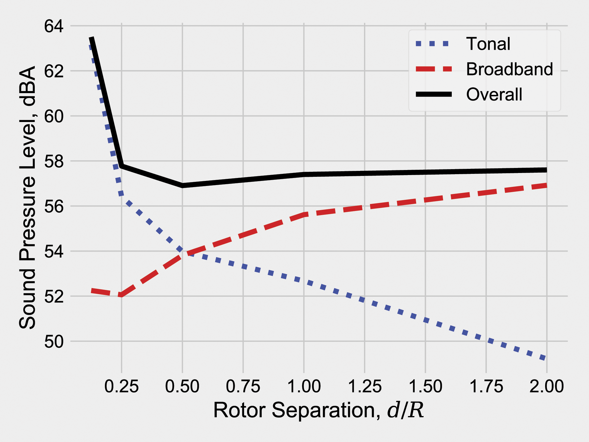
The reason for these trends is more apparent when the measured acoustic signals are filtered to extract the tonal and broadband components of noise. At close separation distances, the tonal noise of the rotors is dominant, but this source of noise diminishes rapidly with increasing separation. However, as the separation distance increases, the broadband noise tends to increase. This is likely due to the breakdown of the rotor wake into nondeterministic structures at long wake ages. Similar trends were observed at the other tip Mach numbers tested (0.2 and 0.3), except that the separation distance for minimum noise increased as the tip Mach number was increased. There are two likely explanations for this trend: (1) tonal noise is relatively more important at higher tip Mach numbers and for the fixed-pitch rotors used; and (2) the increase in thrust causes the wake of the upper rotor to convect to the lower rotor more quickly, resulting in a shorter wake age interaction at the same separation distance.
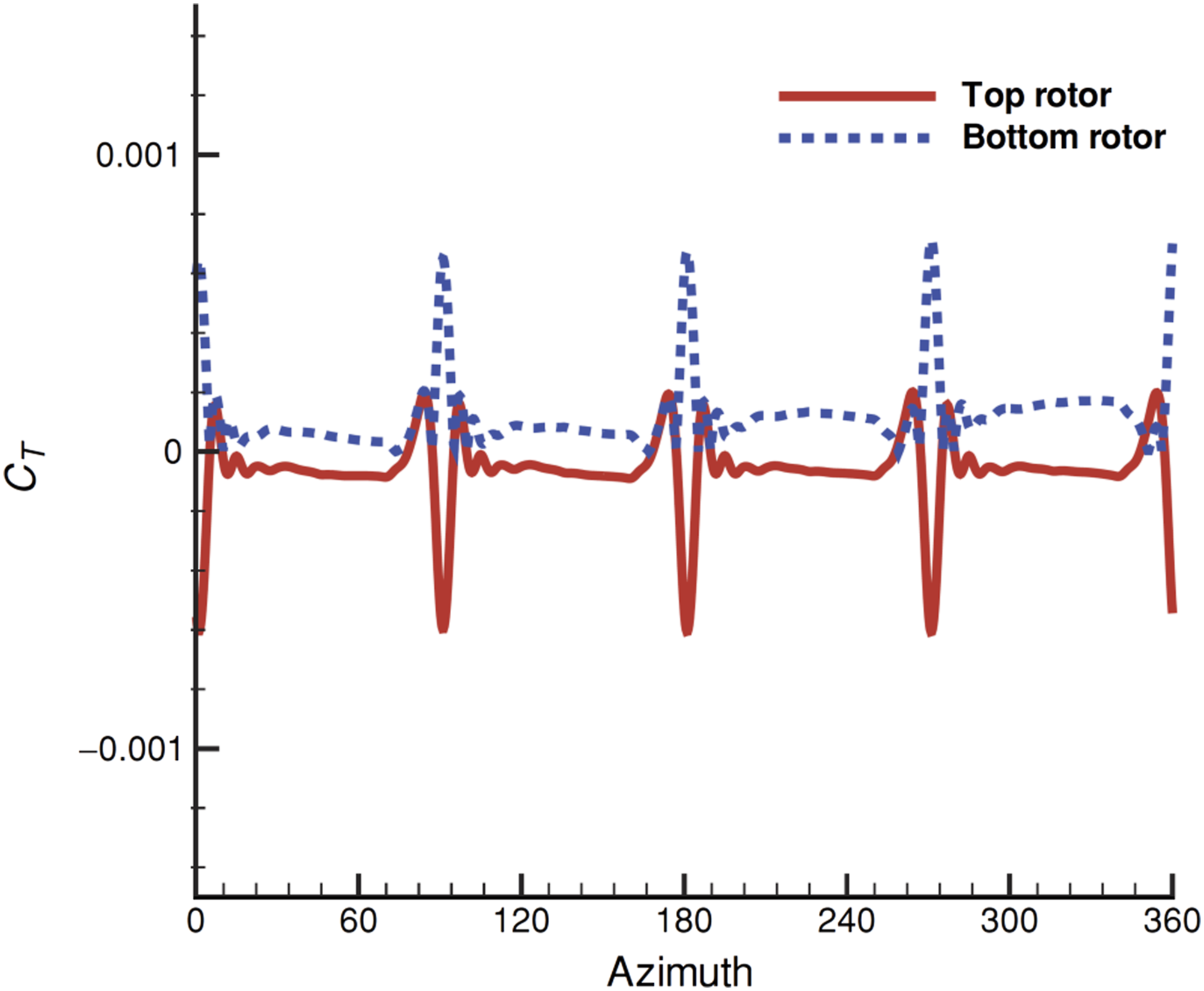
Lakshminarayan and Baeder
74
performed a detailed computational study of the aerodynamic interactions between a pair of counterrotating coaxial rotors with separation distances of 0.16, 0.24, and 0.32 radii. They found that aerodynamic interactions between the rotors generated highly impulsive loading on both the upper and lower sets of rotor blades, which could generate impulsive noise. This loading was caused by two mechanisms. First, in generating lift, each blade induces an upwash ahead of it and a downwash behind it, as would be expected from lifting line theory. As the blades pass each other, they induce a rapid change in angle of attack, somewhat like a blade-vortex interaction. However, strong impulsive loading was observed even when the rotors were trimmed to zero thrust, as shown in Figure 28 for the closest rotor separation of 0.16 R. This is attributed to the displacement of fluid by the rotor blades, which causes a sharp reduction in pressure between the rotor blades when they cross each other. Both effects were found to diminish with increasing separation distance, although the displacement effect diminishes more quickly than the lift-induced effect. Studies of counter-rotating propellers have shown that changes to the blade planform, especially sweep, can mitigate the effect of blade crossover interactions by decreasing the far-field acoustic radiation efficiency.
75
However, when applied to the lower tip Mach number rotors typical of electric aircraft, such as that designed by Coleman et al.,
73
the reductions in radiated noise due to blade planform shaping are more modest than for higher speed propellers. Instantaneous rotor thrust time history at zero mean thrust.
74
Rotor-rotor interactions can be more complex in edgewise flight. Jia and Lee 76 examined rotor-rotor interaction aerodynamics and noise for a lift-offset rotor in high speed forward flight using the high-fidelity rotorcraft simulation software Helios. They also identified blade crossover events as a significant contributor to radiated noise. In addition, in forward flight blade-vortex interactions could also cause unsteady loading noise. Depending on how the vehicle was trimmed, strong blade vortex interactions could occur between a rotor and its own wake (termed “self-BVI”) or between a rotor and the wake of the other rotor. Blade crossover events tended to dominate the impulsive loading of the upper rotor, whereas BVI was more significant for the lower rotor. The relative importance of these interactions depends on both the vehicle flight condition and rotor trim states. Additionally, the most acoustically significant source, unsteady loading varied depending on the azimuthal direction of the observer.
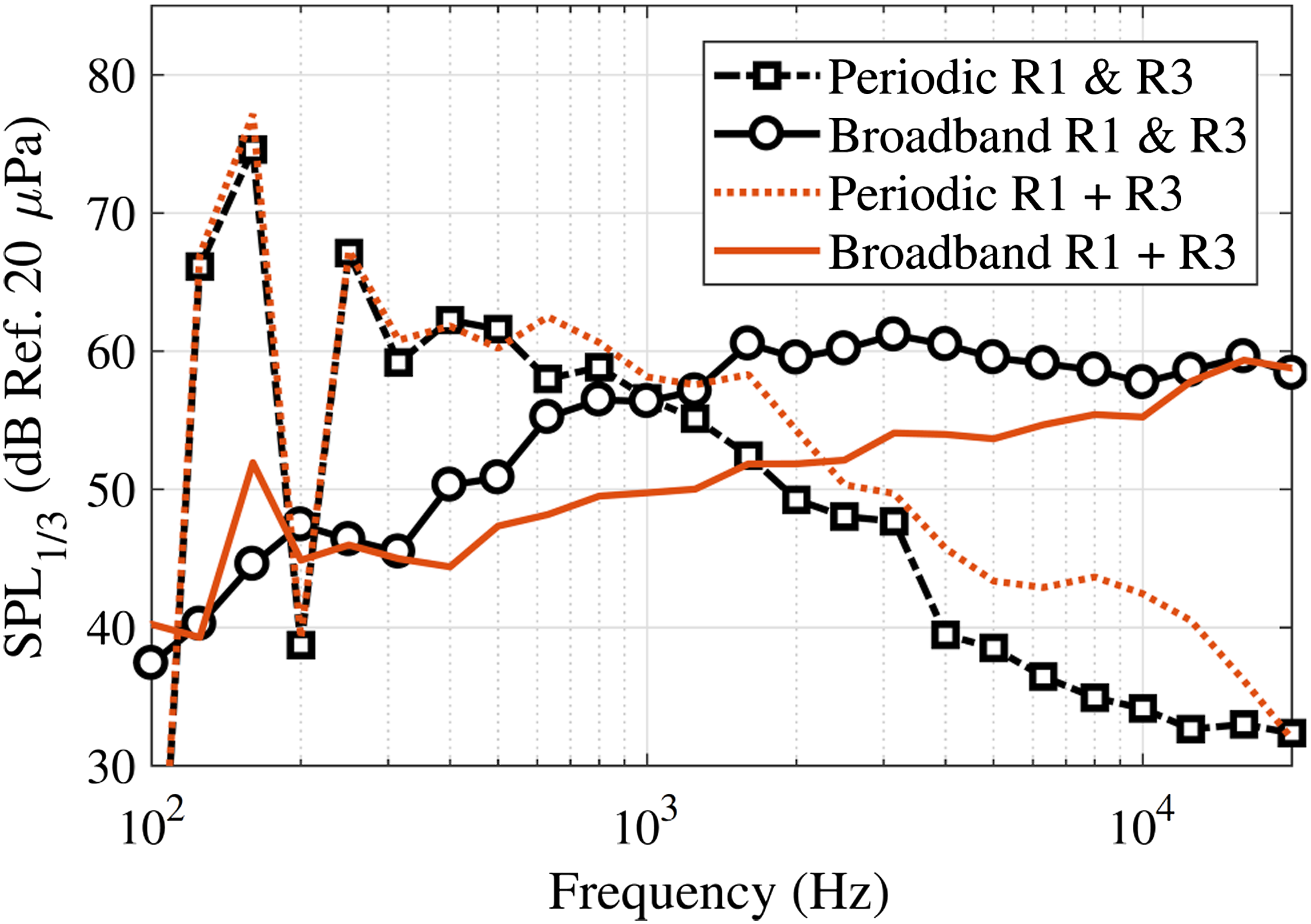
Relatively little experimental or computational data exist for the longer wake age interactions that appear to cause broadband noise. Pettingill and Zawodny
77
conducted one benchmark experiment by collecting acoustic data on an SUI Endurance quadcopter in simulated forward flight in the NASA Langley Low Speed Aeroacoustic Wind Tunnel (LSAWT). In addition to operating the vehicle as a whole, data were collected with individual rotors operating. Figure 29 shows the noise spectra for a fore (R1) and aft (R3) pair of rotors on the quadcopter. The tonal (periodic) and broadband components of the noise have been separated. The lines labeled R1+R3 are produced through the superposition of individual rotor noise measurements, whereas the lines labeled R1&R3 represent measurements of both rotors operating at the same time. Little difference is observed between the tonal noise spectra for the isolated and combined rotors. However, there is a 10 dB increase in broadband noise for both rotors operating together as compared to the superposition of individual measurements. Pettingill and Zawodny attribute this increase to ingestion of the turbulence wake of the upstream rotor by the downstream rotor. Tonal (periodic) and broadband components for interacting (&) and isolated (+) rotor pairs.
77
Rotor-airframe interaction noise
In addition to interactions between the rotors and/or propellers, interactions between fixed airframe components (wings, struts, etc.) and rotating blades can generate unsteady loading noise. Block
78
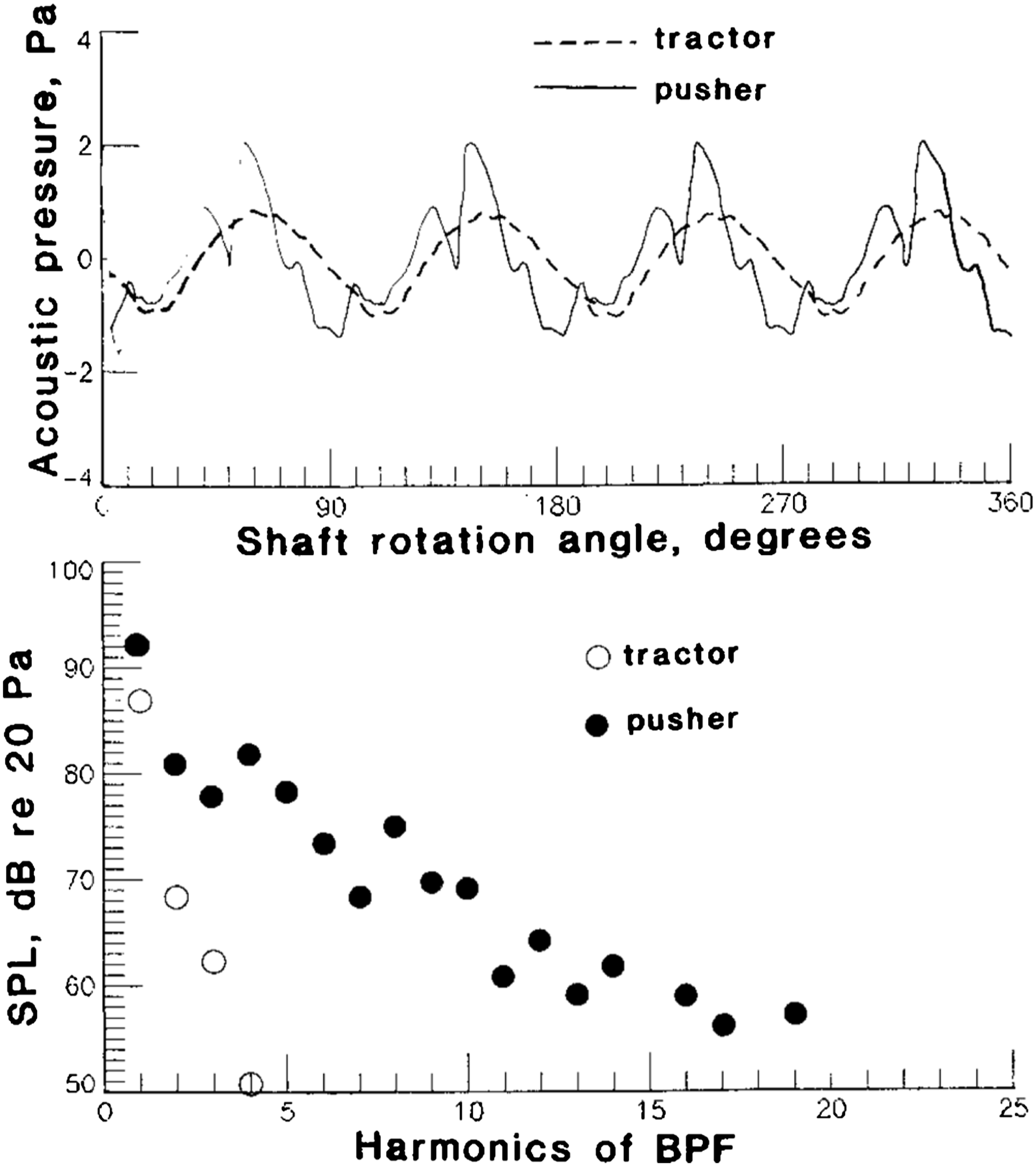
conducted a thorough study comparing the differences in radiated noise for single and counter-rotating coaxial propellers mounted in isolation, in a “tractor” configuration with the propeller upstream of a pylon with a tapered NACA 0012 airfoil cross section, and in a “pusher” configuration, with the propeller mounted downstream of the same pylon. Figure 30 shows a comparison of the measured acoustic data at an upstream observer for a single propeller mounted in both the pusher and tractor configurations. Examing the acoustic pressure time history signals in the upper plot, it is clear that the pusher propeller configuration results in the generation of additional impulsive noise. As shown in the lower portion of Figure 30, these impulses result in an increase in noise at the higher harmonics of the blade passing frequency. Block attributes this increase in noise due to interaction of the propeller with the wake of the non-lifting strut upstream of pusher propeller. More recently, Stephenson, et al.,
79
arrived at similar conclusions as a result of the Aerodynamic and Acoustic Rotorprop Test conducted in the 40- by 80-foot wind tunnel at NASA Ames. (Comparison of acoustic pressure time histories (top) and frequency spectra (bottom) for tractor and pusher propeller installations.
78
In addition to the aerodynamic effect airframe components can have on the rotor, there is growing evidence that acoustically significant unsteady loading can be induced on fixed airframe components by the rotating blades. Johnston and Sullivan 80 conducted an experiment where a wing was placed in the slipstream of a propeller. The wing was instrumented with microphones to measure the unsteady surface pressures. Using smoke flow visualization, the unsteady surface pressure fluctuations were correlated to interactions with the propeller blade tip vortices. Impulsive surface pressure fluctuations were observed on both the upper and lower surfaces of the downstream wing. Depending on the angle of attack of the wing, the surface pressure fluctuations could convect down the wing chord at different rates, such that they could be in or out of phase by the time they reached the trailing edge of the wing. Blade planform shaping may be used to reduce the radiation efficiency of these interactions, 81 in a similar manner as previously described for counter-rotating rotors.
More recently, Lim
82
used the OVERFLOW CFD code to evaluate the aerodynamic interactions between a wing and upstream proprotor on the XV-15 tiltrotor. The wing was found to generate unsteady loading on the proprotor through two mechanisms, one related to the circulation about the wing and the other related to the displacement of fluid about the wing. These mechanisms are the same as those that cause blade crossover interactions, as described in the previous section. Following this work, Zhang, Brentner, and Smith
83
used mid-fidelity aerodynamic models to show that this unsteady loading noise dominated overall sound pressure levels upstream and downstream of the rotor. In addition to the unsteady loading on the proprotor, Lim’s high fidelity calculations
82
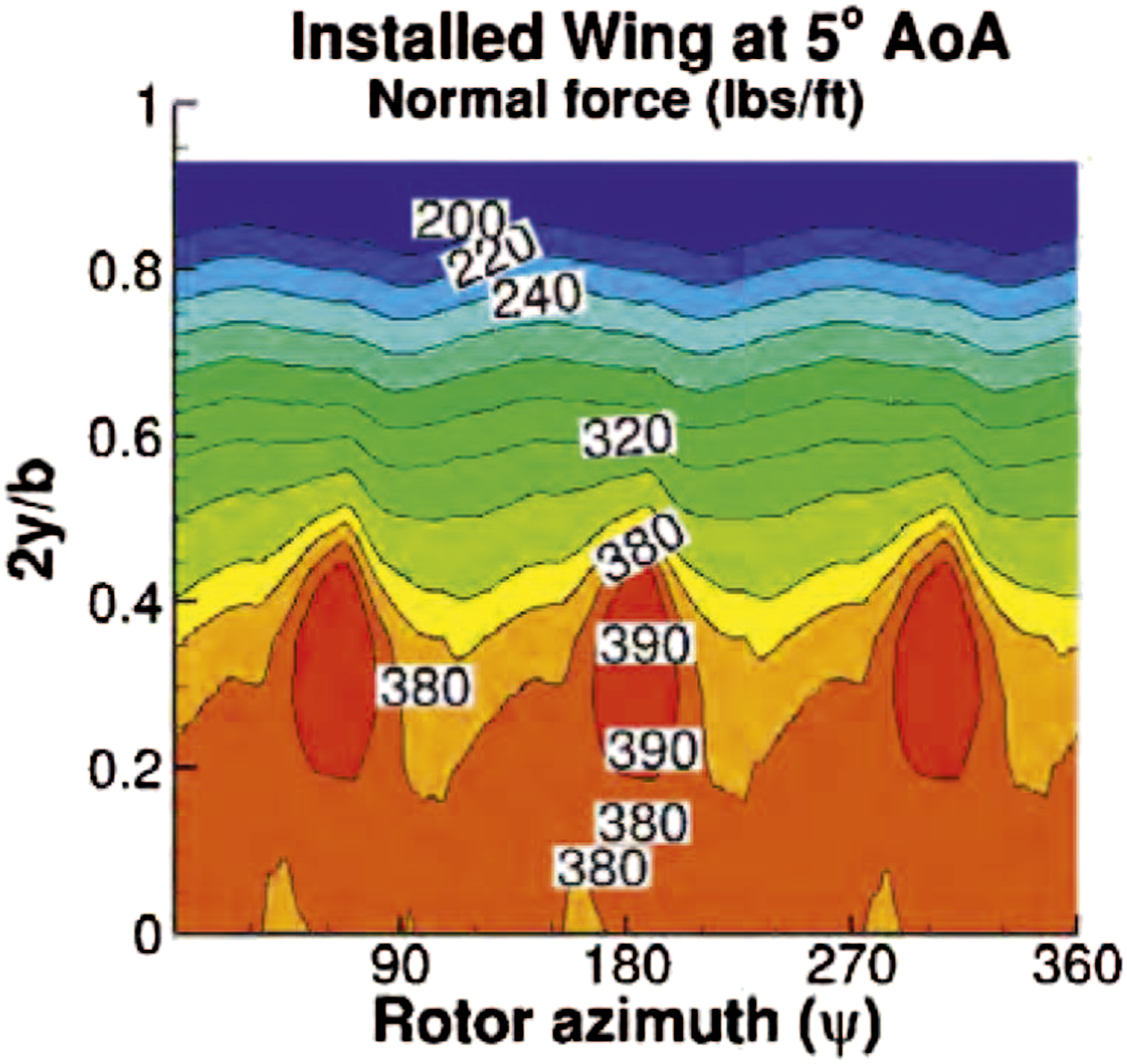
also showed that the rotor generated impulsive unsteady loading on the wing, as shown in Figure 31. Although the wing does not generate noise as efficiently as a rotor blade due to the lack of convective amplification, the high magnitude of unsteady loading combined with the large surface area of the wing could result in significant noise generation. Predicted impulsive loading on the wing of an XV-15 tiltrotor in forward flight.
82
.
Zawodny and Boyd
84
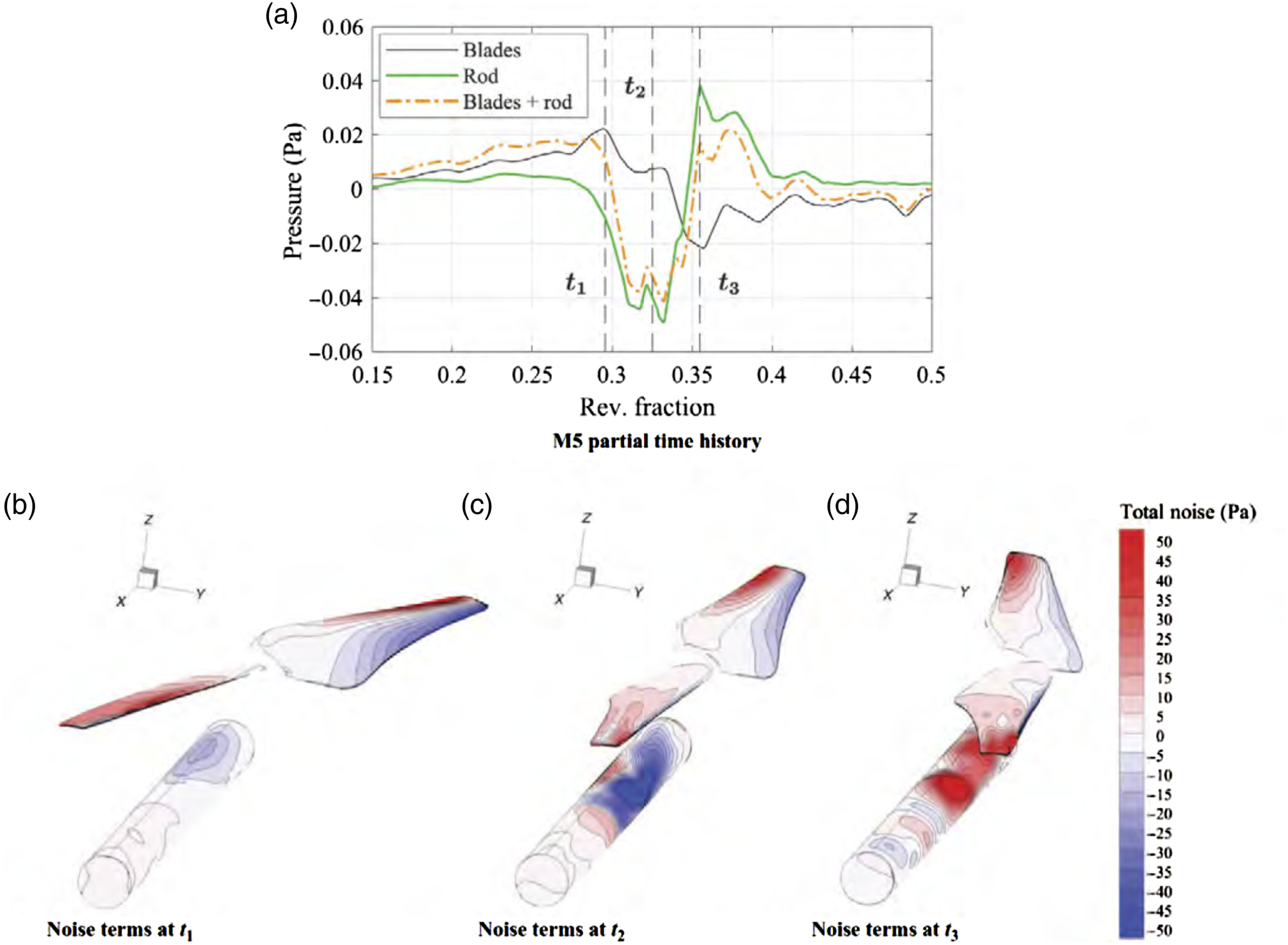
conducted an experiment where a small UAS rotor was operated in hover in isolation, and near simulated airframe components (rods and cones) at various separation distances from the rotor. High fidelity OVERFLOW CFD predictions were also conducted, with excellent agreement between the measured and predicted acoustic pressure time series and levels. Figure 32 shows predictions for a close interaction between the rotor and rod. In the upper plot, predicted pressure time histories are shown for the rotor blades and rod combined, as well as for the separate contributions of the rod and the blades. For this low tip Mach number (0.2) case, most of the noise is generated by the stationary rod. The lower portion of the figure plots a sequence of acoustic data surfaces (Σ-surfaces) showing the acoustic source strengths of the rotor and rod associated with several times of observation marked in the time series plot. The high levels and large spatial extent of the unsteady loading noise generated by the rotor during this interaction are evident. Experiments and calculations were conducted for the rod above the rotor as well, which showed even higher levels of unsteady loading noise generation by the rod due to the sharpness of the pressure field on the suction side of the rotor blades. (a) Predicted acoustic pressure of rotor-airframe interaction for rotor blades, rod airframe, and combined and, (b–d) Σ-surfaces of acoustic pressure associated with different observer times.
84
While this section has primarily focused on the hydrodynamic interactions between rotating blades and fixed airframe components, acoustic scattering or re-radiation of noise generated by the rotors off of the airframe components is more likely to be significant for electric aircraft than conventional rotorcraft. The main rotor blade passing frequency of a conventional helicopter generally corresponds to a wavelength that is large compared to size of the scattering body (fuselage); hence, scattering is not thought to be important in this situation. Even so, there is evidence that scattering of the tail rotor noise can be more significant. 85 Similarly, multirotor vehicles will generate noise with a shorter wavelength relative to the fuselage, which may result in significant scattering of acoustic energy.
Blade-wake interaction noise
Rotor blade-wake interaction (BWI) noise arises from rotor blades interacting with the wake turbulence surrounding tip vortices trailed by the rotor’s own preceding blades.
86
A schematic of this process is shown in Figure 33. Illustration of a blade encountering a turbulent field generated by the other blades of the rotor (Ref. 87).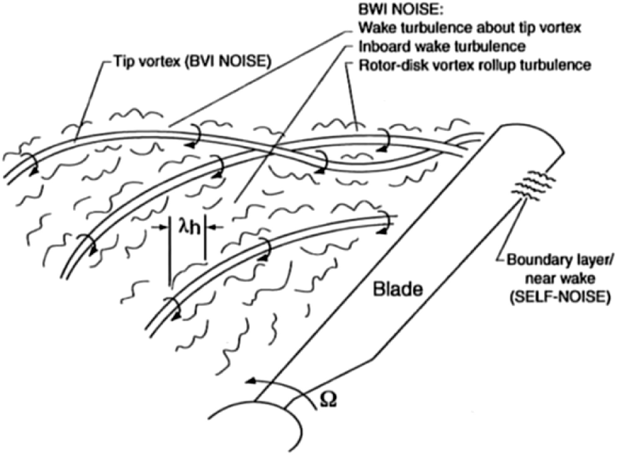
Blade-wake interaction is most important for helicopters in mild climb conditions (see Figure 34). As the climb angle increases, BWI noise is reduced due to the increased miss distance between the vortex and blade. A higher climb angles, self-noise becomes a more important noise source. As described previously, BVI is often the most significant source during descent, although BWI still occurs in these conditions. Regions where main rotor noise sources (BVI/Loading, BWI, Self) dominate for different operating conditions (Ref. 87).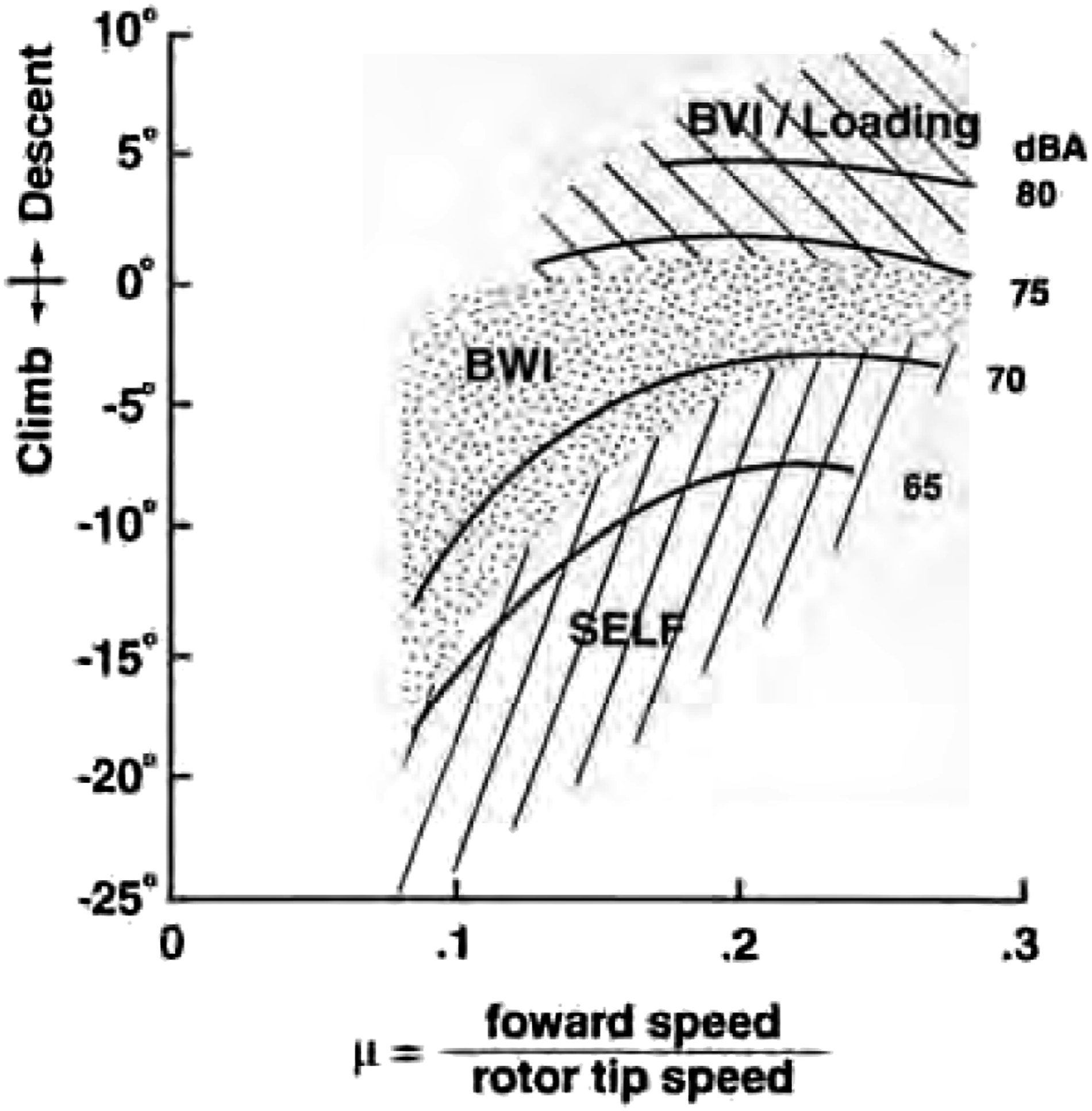
Blade-wake interaction noise is broadband and occurs at frequencies higher than the discrete frequency noise harmonics, but below self-noise frequencies. Although BWI noise is broadband, it is “narrowband random” or “quasi-periodic” in that the broadband noise occurs in bursts (see Figure 35), occurring when the blade encounters turbulence entrained near rotor wake vortices. Although BWI is often characterized using a fixed frequency band,88,89 Vitsas and Menounou demonstrated that such an approach does not differentiate between the higher harmonics of BVI and true BWI noise. The former fluctuations are correlated with BVI noise spikes (Type I fluctuations in Figure 35), while the latter are random (Type II fluctuations in Figure 35).
90
Instantaneous advancing side BVI acoustic signal before (a) and after (b) applying the BWI filter for a single blade passage; fluctuations corresponding to the traditional BWI frequency region are subdivided into Type I and Type II fluctuations in (b) (adapted from Ref. 90).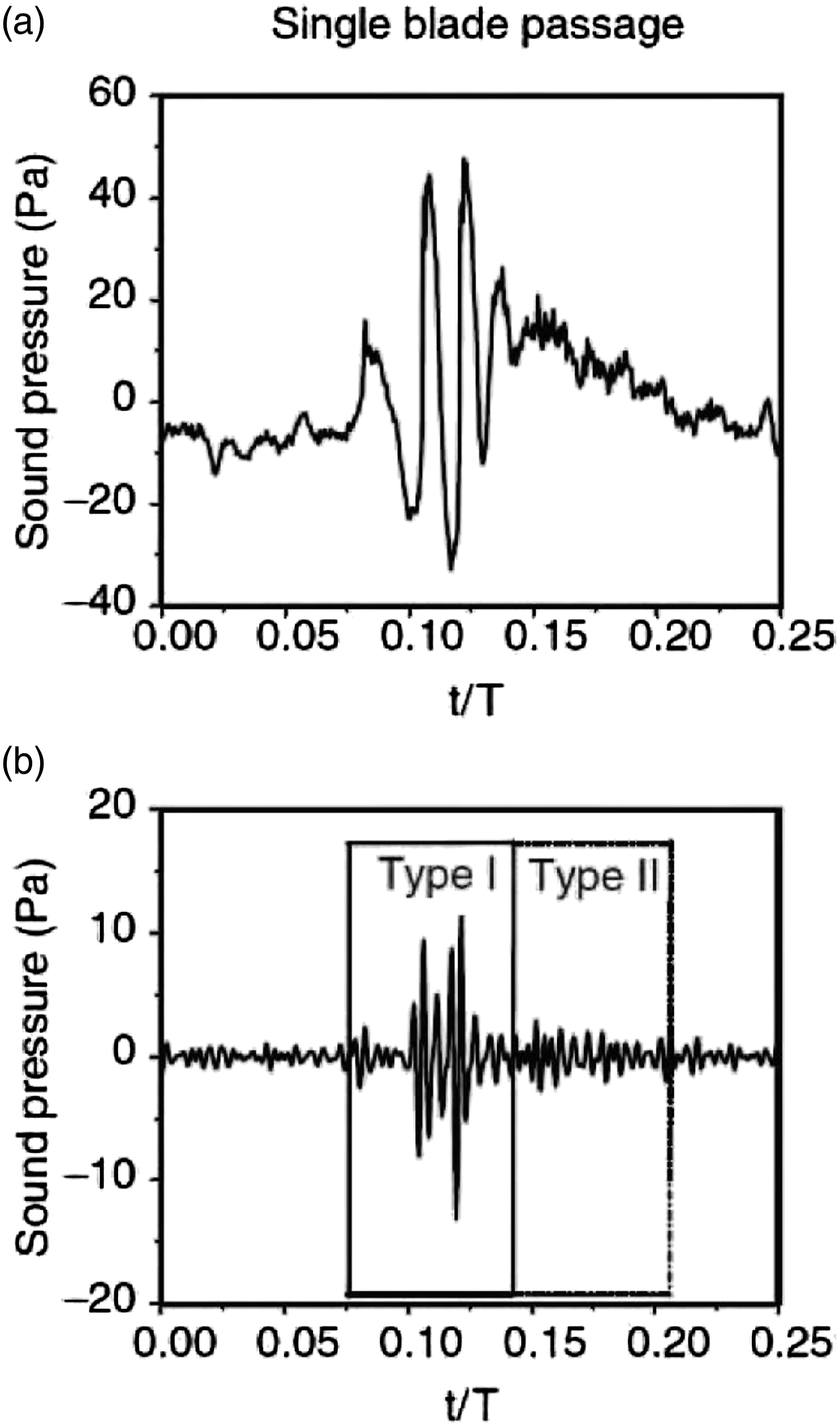
The precise source of the turbulence that causes BWI noise is not well understood. Wittmer et al. 91 conducted an experiment that found that an isolated trailed tip vortex does not generate much noise during a perpendicular BVI. For significant BWI noise to be generated, the tip vortex must interact with a downstream blade to create the intense turbulence required to generate BWI noise in successive interactions. However, Rahier and coworkers demonstrated numerical evidence suggesting that the turbulence causing BWI noise is instead generated by the instability of two co-rotating tip vortices interacting. 92 Despite this disagreement, both theories agree that longer wake ages are required for a tip vortex to become turbulent and contribute to BWI noise. Vitsas and Menounou’s 89 experimental analysis also supports the finding that BWI occurs at longer wake ages.
To the best of the authors’ knowledge, to date, only two known BWI noise prediction models have been developed: by Brooks and Burley, 87 and by Glegg et al. 93 Both are based on leading edge noise prediction models, which typically model blade surface pressure fluctuations induced by wake turbulence, then use those to calculate noise. The Brooks and Burley 87 model takes the surface pressure autospectrum at the leading edge as the primary input. One clear limitation of this model is that the leading edge surface pressure spectrum is not easy to measure, and may not be easily generalized to different operating conditions or rotor geometries. Accordingly, Brooks and Burley recommend that more refined BWI noise models be developed based on wake turbulence statistics, which they consider “difficult but achievable” (Ref. 87, p. 25).
This approach was taken to develop the BWI noise model of Glegg et al.93,94 The inputs into the model are: the turbulent velocity spectrum (modeled based on wind tunnel measurements by Wittmer et al. 91 for the wake of a non-rotating blade that is later ingested by a tip vortex during a perpendicular BVI); the size of the turbulent region (tip vortex and the entrapped shed wake wrapped around the vortex core); and the blade miss distance of the tip vortex center. The latter two inputs were found to be most sensitive parameters on the noise predictions. 93 While the model accurately captured the spectral trends observed in experiments, it under-predicted the noise levels, especially for large tip path plane angles. 93
There have been relatively few studies of BWI noise conducted to date, especially in the last two decades. While a basic framework for BWI noise prediction has been developed, it remains limited by incomplete knowledge of the turbulent structures of rotor wake at long wake ages. However, similar noise mechanisms may be extremely important for eVTOL aircraft due to the high likelihood of similar long wake age interactions. While characterizing rotor wakes at long wake ages remains challenging, new experimental methods and computational tools may provide a path toward understanding and predicting this noise source.
Broadband noise
Airfoil self-noise
Airfoil self-noise was first considered in the context of airframe noise. Initially, it was assumed that airfoil self-noise would follow the U6 scaling 95 of acoustic dipoles 96 (where U is the freestream velocity). However, experimental evidence showed that airframe noise scaled with U5 instead. 97
The first explanation for this discrepancy was presented by the landmark paper of Ffowcs Williams and Hall 2 in 1970. Using a Green’s function approach, they considered the noise of turbulent eddies (modeled as quadrupole sources) scattered by a semi-infinite rigid infinitely-thin flat plate. The inclusion of scattering predicted the now well-known U5 scaling. Although Ffowcs Williams is now better-known for the Ffowcs Williams - Hawking equation, the Ffowcs Williams and Hall solution laid the foundation for modern broadband noise analysis and prediction. An excellent review of broadband noise is provided by Lee et al. 98
Ffowcs Williams and Hall modeled the turbulent eddies as quadrupole noise sources to obtain their solution; whereas, Schlinker and Amiet
97
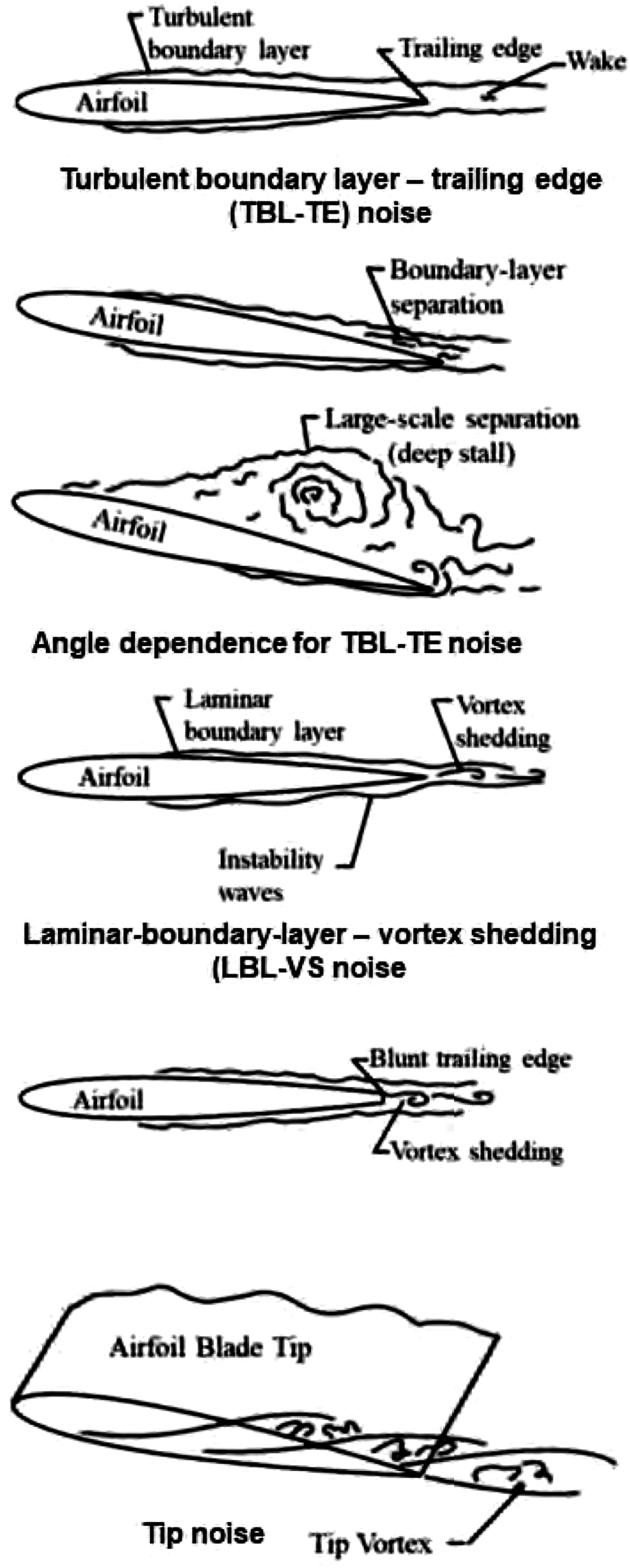
were able to achieve an equivalent result through appropriate modeling of the turbulence-induced surface pressure fluctuations flowing over the airfoil trailing edge as dipole noise sources. This approach of treating noise due to turbulence as being caused by dipole rather than quadrupole noise sources has since been commonly-used in trailing edge noise analysis. Perhaps the most popular trailing edge noise model was developed by Brooks, Pope, and Marcolini,
67
and has thus been commonly-referred to as the BPM model. The BPM model is a collection of empirical and semi-empirical models of different airfoil self-noise sources including: turbulent boundary layer-trailing edge (TBL–TE) noise (or trailing edge noise for short); separation and stall noise; trailing edge bluntness-vortex shedding noise; laminar boundary layer-vortex shedding (LBL–VS) noise; and tip vortex formation noise. These noise sources are visualized in Figure 36. In general, trailing edge noise has received the most research attention compared to the other noise sources. Noise source components predicted by the BPM model (adapted from Brooks, Pope, and Marcolini).
67
The BPM model is based on the Ffowcs Williams and Hall solution of noise due to turbulent eddies scattered by a semi-infinite rigid infinitely-thin flat plate 2 combined with the directivity and Mach number scaling developed by Schlinker and Amiet. 97 The semiempirical BPM model is based on the Strouhal number scaling of analytically-derived similarity spectra, which are then correlated to measured airfoil boundary layer characteristics for the NACA 0012 airfoil.
Although the BPM model was developed for airfoils in steady flow, it is widely-used for rotor noise modeling, as reviewed in Ref. 98, Chap. 5. This implementation for rotors employs many assumptions, outlined in Ref. 99, Chap. 3.2.1. The BPM model is typically implemented for rotors using blade element analysis with a quasi-steady assumption. The noise generated by unsteady flow conditions is computed for different blade elements, with the noise from each blade section at any instant in time being assumed to be equivalent to noise generated by an airfoil in an equivalent steady flow condition. Under this quasi-steady assumption, the BPM model computes a one-third octave spectrum for each blade segment at each instant in time. The noise from the individual blade sections is assumed to be incoherent, so summation of the mean-squared pressures generated by the blade sections is performed to compute the total rotor broadband noise. The accuracy of these assumptions should be assessed for eVTOL aircraft. The blade element assumption neglects spanwise flow, which may be less accurate for highly-swept or low aspect ratio blades proposed on some eVTOL aircraft. The quasi-steady assumption also neglects the time dependent (i.e. hysteresis) effects of unsteady aerodynamics, particularly the unsteady development of the boundary layer. These effects may be especially important where other aerodynamic interactions occur, such as those described in the previous section.
Despite these limitations, the BPM model has been successfully applied to rotors across a range of scales, from helicopter rotors,
86
wind turbines,100–103 and small UAS.77,104,105 Many more examples are outlined by Lee et al. (Ref. 98, Chap. 5). These applications encompass a wide range of chord Reynolds numbers and Mach numbers. The operating conditions of eVTOL rotors are expected to lie within this range, as shown on Figure 37. As will be discussed later in this article, self-noise has been demonstrated to contribute significantly to the time variation of broadband noise spectrum over a rotor period, which is believed to contribute significantly to human perception of helicopter noise.
106
Rotor scales at which BPM model predictions have been successfully-applied.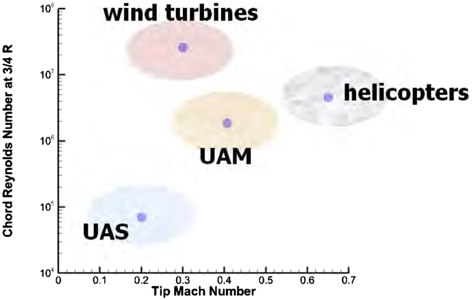
Ingestion noise
Ingestion noise is broadband noise caused by a rotor ingesting turbulence. This turbulence may originate from a variety of sources, such as atmospheric turbulence, or wake turbulence shed by other rotors or airframe components. Blade wake interaction, as discussed previously, may be viewed as a particular form of turbulence ingestion noise. However, the terms “turbulence ingestion noise” (TIN) and “inflow turbulence noise” (the latter of which is often used by the wind turbine noise research community) often imply atmospheric turbulence ingestion; therefore, this article uses the more general term “ingestion noise” so as not to imply the source of the turbulence. Alternatively, Robison and Peake 107 use the term “unsteady distortion noise” to include ingestion of both atmospheric turbulence and upstream wakes, but they also include tonal noise in this term.
Leading edge noise
Fundamentally, ingestion noise is generated by incoming turbulence interacting with an airfoil. Therefore, this noise source is sometimes simply termed “turbulence-airfoil interaction noise”. This noise is generated mostly at the leading edge, and so it is often called “leading edge” (LE) noise. However, recent evidence may suggest that the trailing edge may contribute appreciably to turbulence-airfoil interaction noise.108,109
In 1975, Amiet published a landmark paper 110 that forms the foundation of leading edge noise prediction to this day. Amiet’s approach and its extensions were reviewed by Roger and Moreau, 111 and related to trailing edge noise prediction models. The analytical frequency domain approach employed by Amiet involves decomposing the incident turbulence into harmonic gusts, and integrating over the gust frequencies. The incident turbulent velocity fluctuation statistics are input into an unsteady lift response function obtained from linearized compressible flow assuming small perturbations. This models the surface pressure spectrum induced by turbulence, which is then related to the far-field noise spectrum. Amiet modeled the airfoil as an infinite span, infinitely-thin rigid flat plate in a uniform mean flow at zero angle of attack; therefore, there is zero mean loading, and the plate is at rest or in rectilinear translation in the freestream direction. Frozen isotropic turbulence satisyfing Taylor’s hypothesis is assumed, whereas acoustic compactness is not assumed. Amiet’s work has since been improved to account for realistic airfoil geometries (including non-zero thickness and camber), mean loading (including non-zero angle of attack), non-uniform mean flow, and turbulence anisotropy. Many of these improvements have been summarized by Mish and Devenport, 112 and more recently by Zhong et al. 113
One important area of improvement to Amiet’s work has been considering the effects of realistic airfoil geometries, rather than treating the airfoil as an infinitesimally-thin flat plate. Leading edge thickness has been shown to be an especially-important parameter, as it tends to reduce noise.111,113–115 Since realistic airfoil geometries generate mean loading, they affect the mean flow near the airfoil, and this changes the turbulence statistics. These effects have been studied using a variety of analytical113,116,117 and numerical methods, 117 such as the boundary element method (BEM) and panel methods.118–120 Rapid distortion theory (RDT)121,122 is often used to determine how turbulence is affected by irrotational mean flows, and the resulting effects on noise.116,118–120,123,124
The effects of non-uniform mean flow upstream of the airfoil represent another important extension to Amiet’s work. As before, the effects of non-uniform mean flow upstream of the airfoil can also be studied using RDT, provided that the mean flow is irrotational. To determine the effects of rotational mean flows, one could use Goldstein’s extensions of RDT to mean shear flows.125–129 However, to apply these techniques, the mean flow must still be parallel and homogeneous in the streamwise direction, 127 the latter of which may pose an issue for ingestion noise.
Ayton and Peake 108 applied Goldstein’s RDT extension for rotational flows to find that mean shear caused significant noise level increases and noise directivity changes compared to uniform flow. Gershfeld 115 also studied leading edge noise of an airfoil in constant mean shear (i.e. a triangular velocity profile). Gershfeld found that there exists a critical frequency below which loading noise due to mean shear dominates over loading noise due to a uniform mean flow.
Non-uniform mean flows, whether upstream or near the airfoil, generally cause turbulence anisotropy. The effects of turbulence anisotropy on leading edge noise have been reviewed and studied recently by Gea-Aguilera et al.130,131 and by Zhong and Zhang. 117 The effects of angle of attack 116 and camber have been found to be small for isotropic turbulence.111,131 However, as reviewed by Roger and Moreau, 111 it is unclear if this conclusion also holds for anistropic turbulence.112,130,132
As discussed in the helicopter noise review paper of Brentner and Farassat, 133 an alternative to Amiet’s approach would be to calculate sound propagation directly using the Ffowcs Williams and Hawkings equation. Note that this requires the nondeterministic loading to be known. While Farassat’s Formulation 1A is commonly used for deterministic noise prediction, 133 it has not been widely used for the prediction of nondeterministic noise. However, Farassat developed Formulations 1B 134 and 2B 135 specifically for broadband noise computations. These formulations may be useful if detailed time domain loading data are available, for instance from high fidelity computational tools such as those described in the next section. However, Formulations 1B and 2B have not seen much use since their development 136 and should be compared to Formulation 1A to assess their relative accuracy and computational efficiency.
Atmospheric turbulence ingestion noise
Although ingestion noise is LE noise, there are a few special considerations involved when applying LE noise methods developed for airfoils to rotors. These include the changes in turbulence caused by rotor inflow, blade rotation effects, and blade-to-blade correlation. Historically, atmospheric turbulence ingestion noise has received more attention for helicopter main rotors compared to wake ingestion noise, which is described in the following section.
A general approach to atmospheric turbulence ingestion noise is based on the work of Amiet and coworkers137,138 applied to helicopter rotors. In this model, the turbulence is assumed to be statistically stationary. Far upstream of the rotor, the mean flow is assumed to be uniform, and the turbulence is assumed to be isotropic.
137
Although the turbulence is isotropic upstream, it becomes anisotropic near the rotor disk plane; this is due to the stretching of eddies (and thus the turbulence length scale) in the rotor axial direction due to inflow streamtube contraction.139,140 This effect can be predicted using rapid distortion theory,
137
which is possible because the mean flow is assumed to be uniform upstream of the rotor. Accounting for this turbulence anisotropy greatly improves predictions compared to assuming isotropic turbulence near the rotor disk plane,137,138,140 even though the anisotropy is simply modeled by stretching the turbulence length scale of isotropic turbulence by a scalar factor in the rotor axial direction.
140
The general approach taken by Amiet and coworkers is illustrated in Figure 38. This prediction framework is similar to future studies of ingestion noise undertaken by other authors, e.g. by Robison and Peake (Ref. 107, Figure 2). Modules in overall prediction scheme for atmospheric turbulence ingestion noise of rotors (Ref. 137).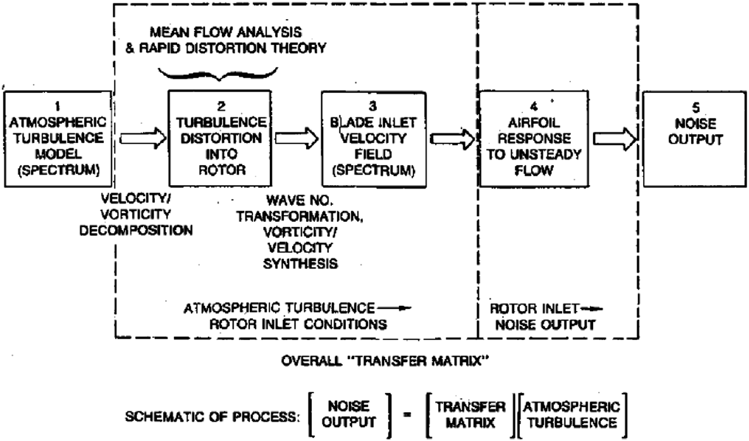
Another important consideration for ingestion noise not present for airfoil leading edge noise is the added effect of blade rotation, discussed by George and Kim 141 and by Roger and Moreau. 111 Amiet justified treating the ingestion noise of rotating blades as if the blades were in rectilinear motion, by assuming that the acoustic frequencies are much larger than the rotor frequency.142,143 This allows ingestion noise to be treated in a “blade element theory”-like (or strip theory) approach by summing the LE noise from different blade sections treated like airfoils in rectilinear motion, and averaging the noise over a rotor period, with consideration of retarded-time effects. 142
An important consideration during this “blade element” summation is blade-to-blade correlation.
141
This occurs due to blades repeatedly interacting with the same turbulent eddy. This can generally occur for helicopter rotors (despite their low solidities) because eddies are stretched by the rotor’s inflow streamtube. Blade-to-blade correlation causes “haystacking” in the noise spectrum, in which the noise is spread out into near spectral peaks139,140; this is sometimes termed “narrowband random noise”. Note that edgewise flight causes non-axial mean flow. This spreads out the narrowband random spectral peaks, and shifts the frequencies away from the blade passage frequency harmonics,
144
as shown in Figure 39. Effect of skewed inflow (forward flight) on narrowband random noise peak frequencies (Ref. 144).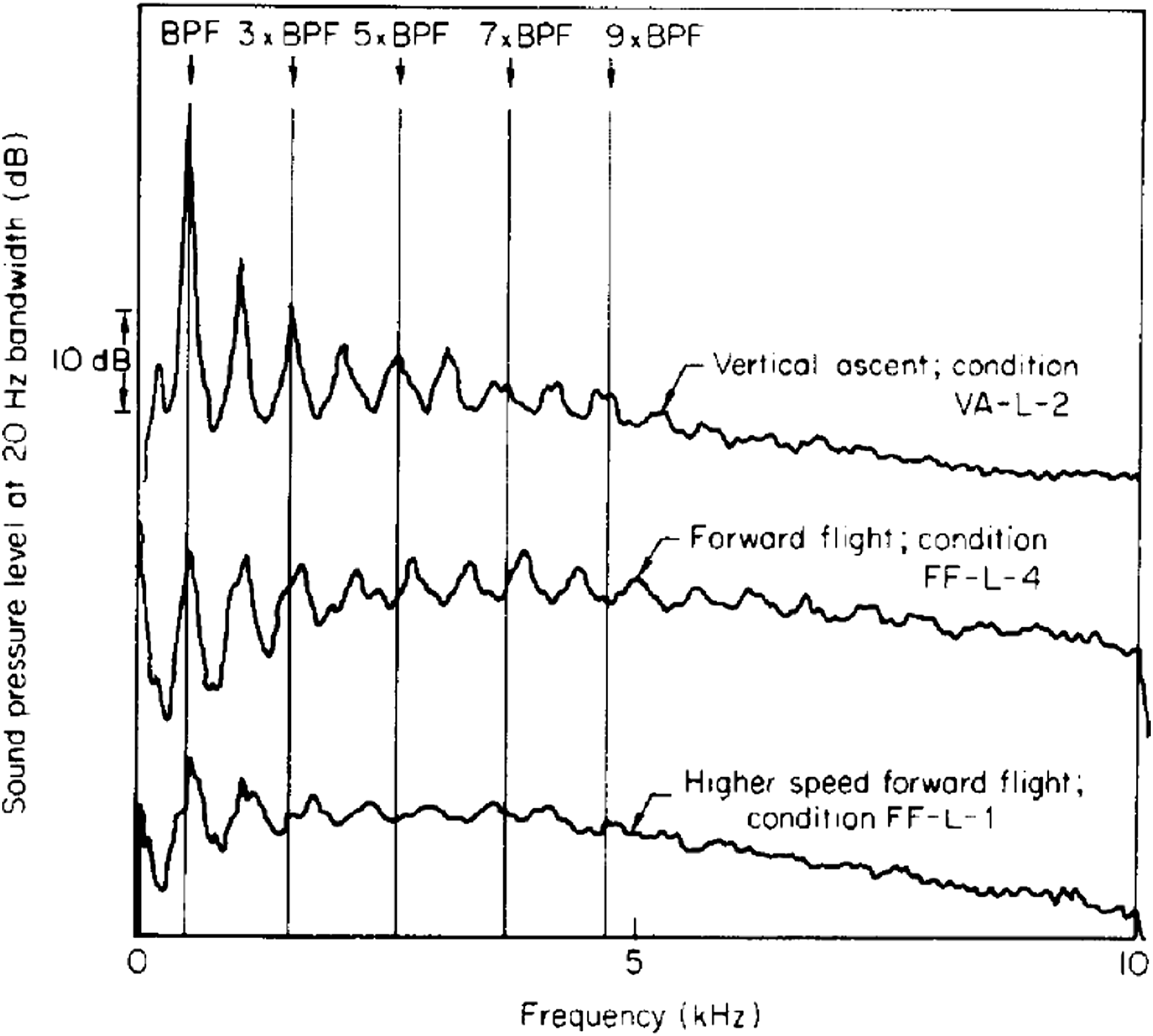
Since the work of Amiet and coworkers, helicopter noise due to turbulence ingestion has not received much attention, as broadband noise in general is not usually emphasized for helicopters, due to dominance of discrete frequency noise sources, such as BVI noise. However, it is likely to be a significant contributor to eVTOL noise, for the same reasons that other sources of nondeterministic loading noise are likely to be of elevated importance. Atmospheric turbulence ingestion is likely to be particularly significant during hovering flight conditions, where other aerodynamic interactions are likely to be minimal for a well designed configuration.
Wake ingestion noise
Rotors may not only ingest atmospheric turbulence, but wake turbulence shed by other rotors or airframe components. In contrast to atmospheric tubulence, wakes are unsteady, non-axisymmetric, rotational mean flows, with turbulence that is inhomogeneous, non-stationary, and anisotropic.
Wake ingestion noise has received particular research interest for aircraft turbomachinery, including recent trends such as boundary layer ingestion into propulsion devices145–147 and contra-rotating open rotors.107,148,149 The suitability of such existing noise prediction models for wake ingestion noise of eVTOL aircraft must be evaluated. However, caution should be taken when applying this research to aircraft rotors and propellers. Factors to consider include: (a) periodicity, (b) the extent of axial and edgewise flow, (c) the effects of ducts, (d) rotor solidity, and (e) blade-to-blade correlation. The high blade counts used in turbomachinery may lead to simplifications,107,150 or as noted by Roger and Moreau, 111 may change the noise prediction approach altogether, towards the use of cascade response functions.151,152 Different rotor solidity, rotational speed, and thrust values may also affect the extent of blade-to-blade correlation.
Wake ingestion noise may be especially important for eVTOL aircraft, as their novel geometries create increased opportunities for aerodynamic interactions, which increase the likelihood of wake ingestion. Therefore, future research especially-relevant for eVTOL aircraft include the effects of anisotropy and mean shear flow on leading edge noise. The literature reviewed in this section has already started to address these fundamental issues. Future work should continue applying these LE noise findings to rotor ingestion noise research.
Robison and Peake 107 compare and contrast frequency domain approaches for predicting LE noise to time domain approaches making use of velocity correlation functions (e.g. used by Refs. 145,153,154). Robison and Peake 107 discuss how frequency domain approaches are well-suited to known turbulence spectra (e.g. atmospheric turbulence spectra), whereas time domain approaches may be better-suited to measured correlation functions. One important fact noted by Robison and Peake 107 is that the effects of mean flow on turbulence are typically analyzed in the frequency domain (e.g. rapid distortion theory and its extensions to rotational flows). Time domain (or perhaps time-frequency analysis) methods may be particularly suitable for the time-varying nature of eVTOL noise, due to the unsteadiness, aperiodicity, and non-stationarity inherent to the aerodynamics of eVTOL aircraft.
Experimentalists studying the noise of unmanned aerial systems (UAS) take caution to ensure that noise due to recirculation of their own turbulent wake does not dominate noise measurements conducted in enclosed areas.155–157 That research, along with other recent research,158,159 suggest that ingestion noise can contribute significantly to UAS noise. Thus this is an important area for future research, which could also have some relevance for eVTOL aircraft.
In summary, although there exists numerous aforementioned challenges in predicting the ingestion noise of eVTOL aircraft, this enables many research opportunities. First, the relative importance of broadband ingestion noise compared to other broadband and discrete frequency noise sources should be evaluated (e.g. as is done in Ref. 81). Furthermore, how well existing ingestion noise prediction methods perform when applied to eVTOL aircraft should be evaluated. Performing such research would help determine whether current ingestion noise models need to be improved, and/or whether new prediction methods must be developed.
Challenges and opportunities
Opportunities exist for rotor broadband noise reduction. Popular passive noise control methods for reducing leading and trailing edge noise involve blade surface geometry modifications. These include serrations or waviness (e.g. see the owl-inspired curved leading edge serrations in Figure 40),160–162 as well as porosity.163,164 See the review of Lee et al.
98
for more detail on these noise reduction mechanisms. Curved-serrated leading edge attached to a wing model (Ref. 161).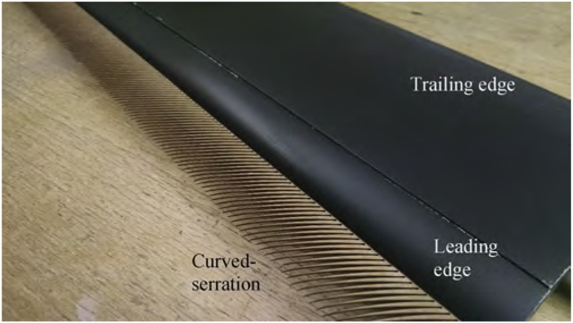
Since trailing edge noise is caused by interactions of turbulence with the trailing edge, delaying or even preventing laminar-turbulent transition would presumably reduce trailing edge noise. Laminar flow can be achieved using specialized airfoils and/or surface treatments. However, a major challenge in studying these noise reduction mechanisms is that popular existing models (e.g. the BPM model) likely do not model the necessary physics needed to evaluate these noise reduction mechanisms. Recall that the empirical scaling of the BPM model was based on the NACA 0012 airfoil. Although the empirical boundary layer correlations of the BPM model are often replaced with data for airfoils aside from the NACA 0012 (as reviewed by Gan in Ref. 99, Chap. 3.2.1), this does not necessarily increase the accuracy of the BPM model. Accordingly, higher fidelity models could be used. The wall pressure spectrum of the turbulent fluctuations near the trailing edge could be modeled. However, these wall pressure spectrum models often require boundary layer parameters as input: e.g. displacement thickness, edge velocity, pressure gradient, etc. 98 Although these parameters may be obtained using Reynolds-averaged Navier-Stokes (RANS) computational fluid dynamics (CFD) simulations, higher fidelity large eddy simulation (LES) or direct numerical simulation (DNS) are becoming increasingly accessible as computational capabilities continue to improve with time. Computing noise using high-fidelity CFD methods is discussed in detail in the following section.
Computational aeroacoustics
Departure from comprehensive computational aeroacoustics
In 1992, James Lighthill declared that aeroacoustics was at the start of a second golden age, with technological advancements opening new opportunities for modeling, simulation, and experimentation, which must be leveraged to meet increasingly strict noise requirements. In Lighthill’s words: “If acousticians can rise to this exacting challenge, communities all over the world will benefit from huge shrinkages in aerodynamic-noise ‘footprints’.” 165
With the rising prevalence of eVTOL aircraft, the situation today looks very similar. At the time, Lighthill strongly urged a two-pronged effort in the computational domain: one that expands on acoustic analogy (or hybrid computational aeroacoustics) approaches, typically in the form of the FW-H equation; and one that expands on what Lighthill refers to as comprehensive computational aeroacoustics (CAA), also referred to as direct noise computation (DNC). The latter consists of computational methods that aim to solve both the bulk flow physics and acoustic field. Nearly 30 years later, comprehensive CAA does not see many applications in rotary wing aeroacoustics, let alone eVTOL aeroacoustics. However, emerging eVTOL configurations stretch the capabilities of our current prediction tools. Aspects such as variable RPM, multiple rotors in lift and cruise configurations, and low tip speeds pose new challenges for computational scientists. 165
Comprehensive CAA aims to solve both the bulk flow as well as the acoustic field using a unified approach. This can allow for the prediction of coupled flow-acoustic interactions, nonlinear wave propagation, refraction, diffraction, shadowing, scattering, and more. Many of the techniques developed for comprehensive CAA have made their way into acoustic analogy approaches that use CFD: correct local dispersion, propagation, and non-reflecting boundary conditions are still seen in acoustic analogy predictions.166,167 However, there are many limitations to performing full domain comprehensive CAA that have slowed its adoption in the rotorcraft community. For eVTOL aircraft, the primary areas of interest for noise prediction are typically in the acoustic far field. This is in contrast to work being done on cabin noise due to air conditioning systems where there is significant scattering and the observer may be in the near field. 168 The use of comprehensive CAA approaches requires discretizing the domain up to the points of interest, or at the very least, up to the start of the far field. Furthermore, the magnitude of acoustic perturbations p′ is much smaller than that of the bulk quantities. This presents practical computational problems due to the precision of floating point numbers, with p′ often being of similar order of magnitude to numerical error of bulk quantities. 169
Acoustic analogy approaches
In a testament to the long lasting impact of Ffowcs Williams, the rotorcraft community has long leveraged the FW-H equation acoustic analogy approach to predict the acoustic impact of the vehicles. Using the FW-H equation avoids many of the issues outlined for comprehensive CAA, but has its own limitations discussed below. Propagation distances are no longer a concern for the FW-H equation, as solutions can be computed for any distance in roughly constant time. Since only the acoustic perturbations are propagated, the issue of scale separation with bulk flow quantities is avoided. Moreover, the lack of time integration removes floating point error accumulation seen in time marching techniques. 1
Most rotorcraft noise computations use an on-surface formulation of the FW-H equation, where the data surface of integration is chosen to coincide with the physical surfaces (e.g. rotor blade). On-surface methods perform well when the majority of the noise generation is caused by thickness (monopole) and loading (dipole), so that the quadrupole (volumetric) sources can be neglected. 133 For conventional rotorcraft at low speeds, this works well, as most noise generation occurs on surfaces, but for flows with off-body shocks or substantial turbulent mixing, this approach falls short. Further, the on-surface formulation fails to capture acoustic scattering effects, shadowing or reflections caused by the body, as well as refraction and diffraction. With the increased importance of broadband noise for eVTOL vehicles, the on-surface formulation may no longer be adequate.
The permeable surface formulation places a fictitious surface in the flow off the body, so that the effect of quadrupole noise sources contained within the surface can be captured. This form of the FW-H equation largely sees applications in jet noise, airframe noise, and the high speed impulsive noise of rotorcraft, where the majority of sound generation occurs off-body. Permeable surfaces capture quadrupole noise through the monopole and dipole terms by entirely enclosing the off-body noise sources with a permeable data surface. This surface is then integrated over obviating the need for integrating the whole volume. Furthermore, by enclosing all noise sources and vehicle geometry, permeable surface formulations can capture many of the effects of included in comprehensive CAA, such as acoustic shadowing and reflections off the vehicle, as well as near-field nonlinear propagation effects. This removes the need to extend the computational domain out to the acoustic far field, assuming appropriate CFD methods are chosen. This strikes a middle ground between comprehensive CAA and on-surface FW-H. However, permeable surface FW-H is formulated such that all noise sources are contained in the surface.
3
If flow features such as vortices pass through the surface, spurious acoustic signals arise. Lopes et al. studied this effect by setting up a cubical domain with a point monopole source and passing a non-deforming vortex ring through the permeable surface. This setup can be seen in Figure 41. Figure 42 shows the time evolution of the acoustic field inside the domain as the vortex passes through the surface. They concluded that while the permeable surface removes the need to integrate over the inner volume, the outer volume still needs to be integrated to account for the flow features outside the surface to properly remove spurious signals.
170
This study provides concise numerical experiments demonstrating the care needed to properly use permeable surfaces. Computational setup of the model problem of Lopes et al. (Ref. 170). A series of time snapshots showing the acoustic pressures inside the surface. (a) also shows the observer grid used (Ref. 170).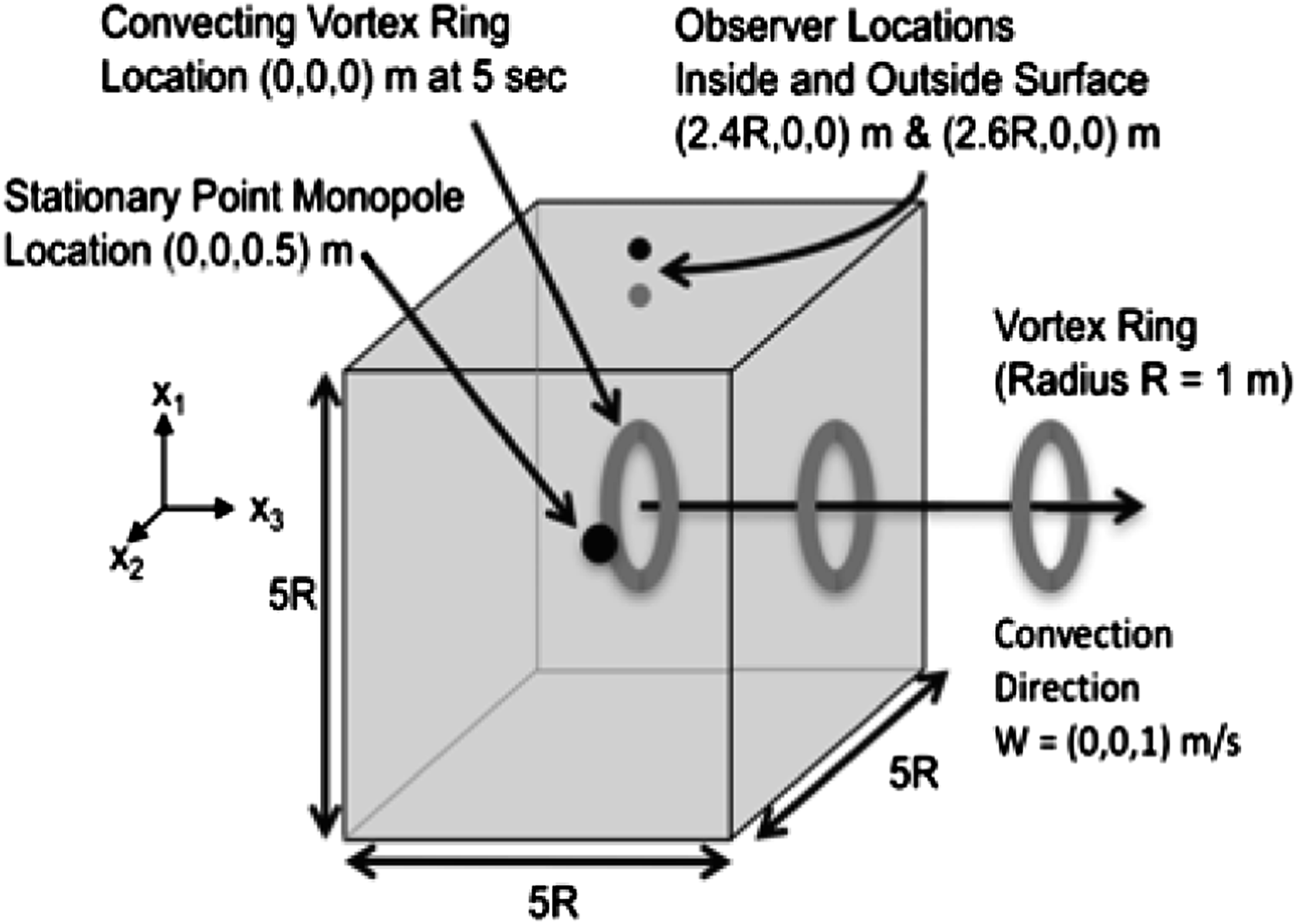
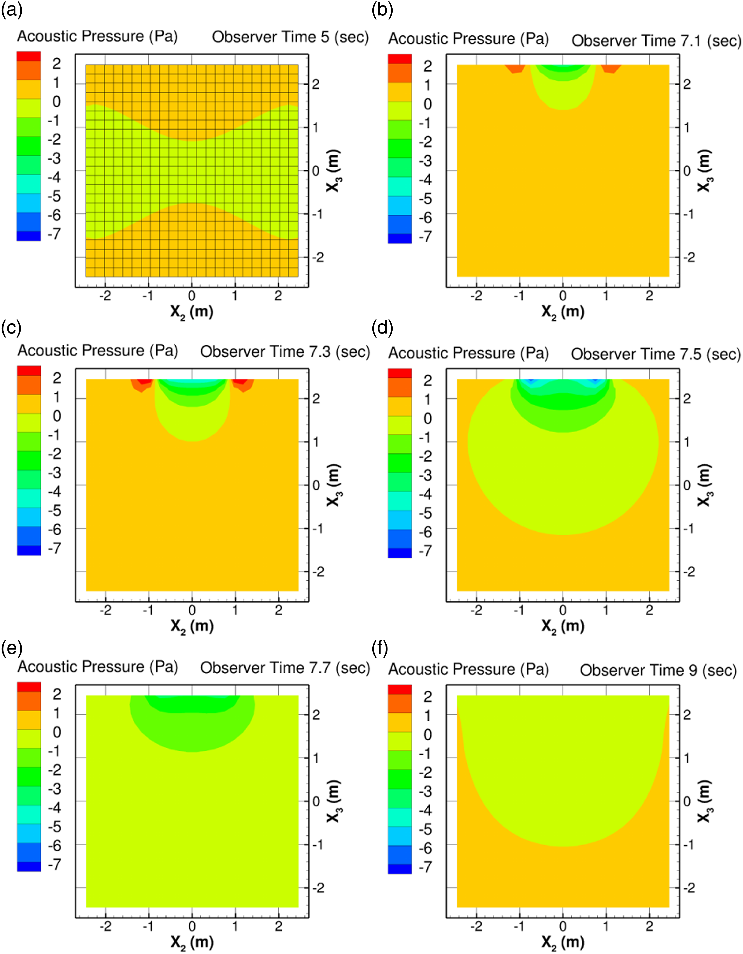
A series of numerical experiments by Spalart et al.
171
demonstrated the usefulness of the permeable surface formulation in spite of its apparent deficiencies. In one such case, a box was placed in a flow with a permeable surface placed around the box. This can be seen in Figure 43, where there are three end-caps at different downstream stations. The data at each of these end caps is averaged together for the final acoustic propagation. It was shown that for such a case, on-surface FW-H is not sufficient to capture all of the acoustic physics present in the scenario. This can be seen in Figure 44, where the on-surface formulation not only underpredicts SPL at high frequencies, it also exhibits incorrect Mach number scaling. It was noted that with good engineering judgment, smart placement of the permeable surface can generate good results without generating too much spurious noise. While this study was for airframe noise of large commercial aircraft, eVTOL configurations can expect to have many airframe configurations with rotor wakes impinging on both different rotors as well as the body. In conjunction with lower tip speed and quiet motors, these turbulent off-body noise sources may become more important in the future. Computational setup of Spalart et al. permeable surface experiment. White dots are the two microphone locations (Ref. 171). Results showing the acoustics missed by the on-surface formulation with θ = 0° being the upstream microphone and θ = 90° being the top microphone (Ref. 171).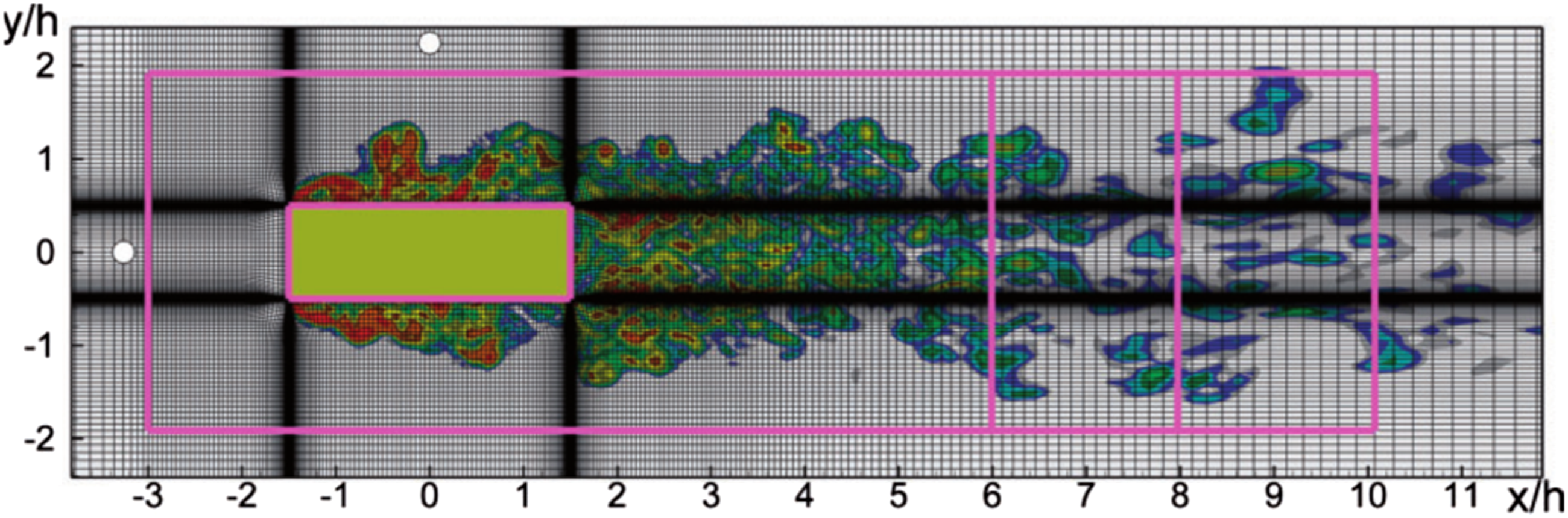
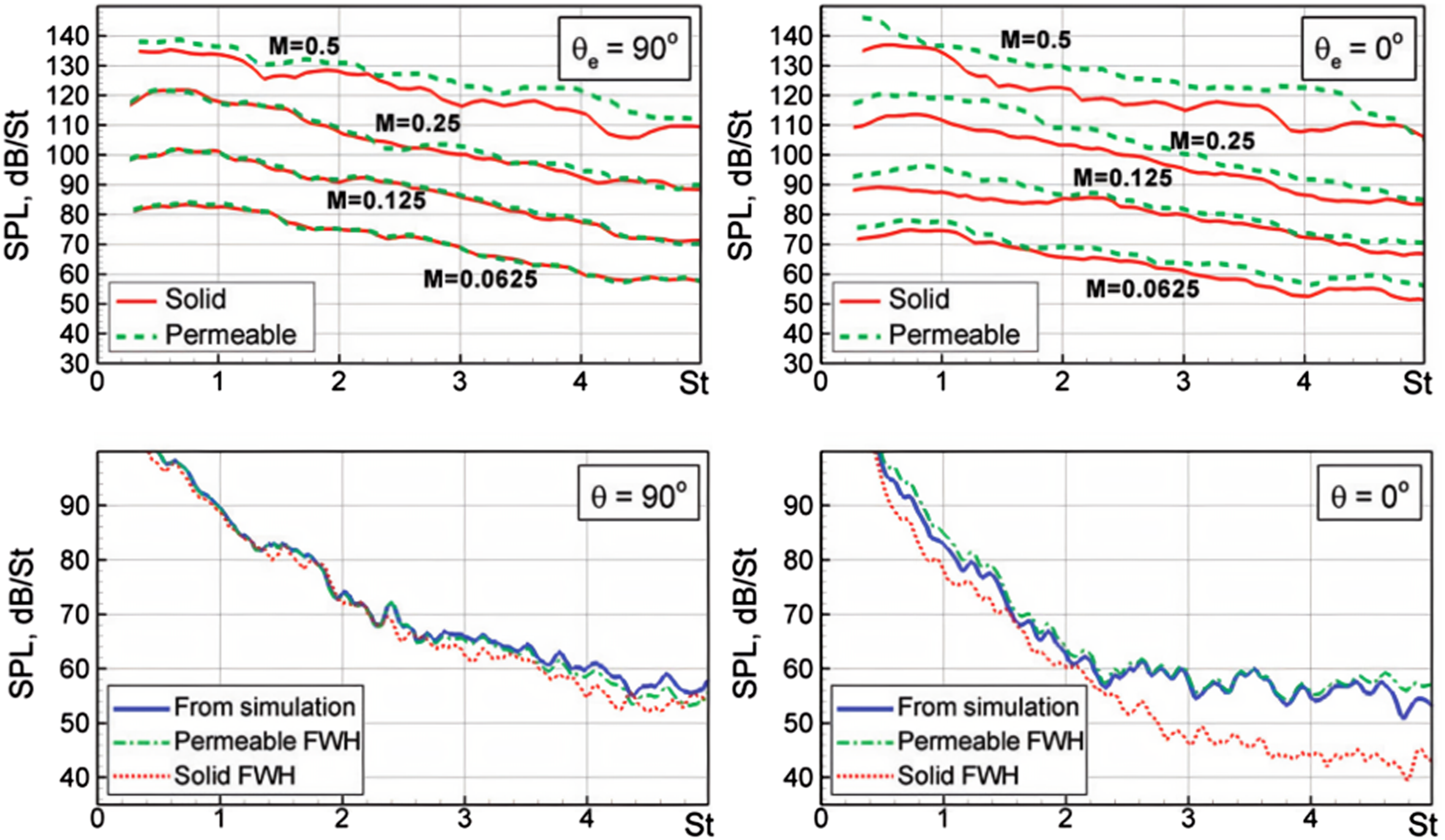
Challenges
Wake prediction
One of the key challenges to prediction of helicopter noise is adequate wake prediction. Simple models can accurately predict thickness and steady loading noise, but accurate prediction of wakes is required to model unsteady loading sources such as BVI. Not only does this remain true for eVTOL the problem is even more complicated due to the long wake ages associated with many interactions.
Of course, accurately simulating a long-lasting wake is a challenging proposition for CFD. It requires that there be minimal numerical dissipation as the wake convects downstream. The trajectory and intensity of this wake are important to the overall vehicle sound, especially if that wake interacts with a rotor. Wang et al.
172
conducted numerical simulations on a model problem of the wake of a cylindrical strut impinging on an open rotor. Figure 45 shows that as the wake interaction point moves closer to the center of the rotor, the sound levels produces increase. They do not, however, increase at the same rate for each microphone, meaning that not only does the overall sound level increase, but the directivity changes as well. The effects of wake interaction location on sound levels at different microphone locations. 100% off-center (—); 75% off-center (- - -); centerline (......) (Ref. 172).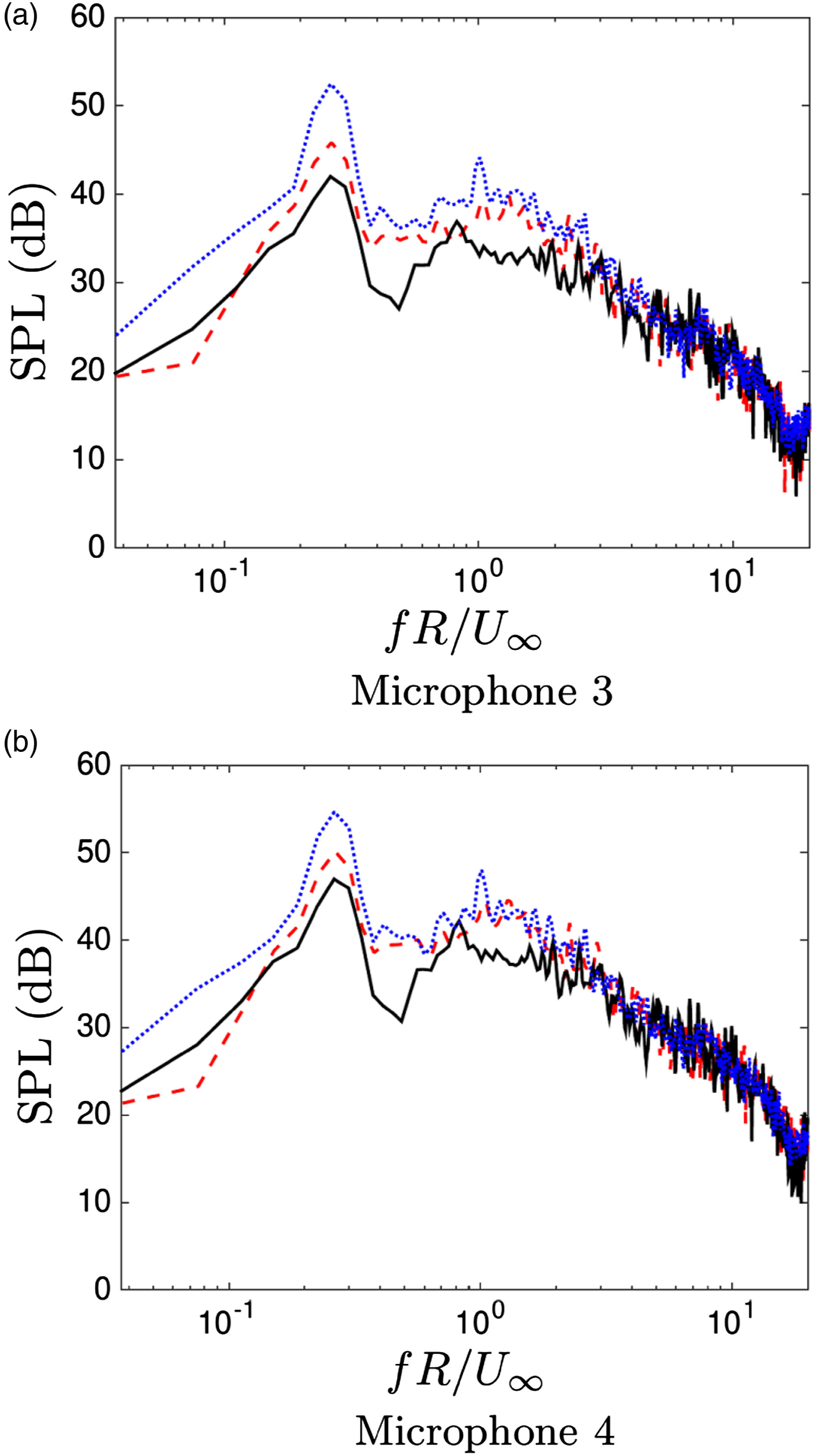
Broadband noise
As mentioned previously, lower tip speeds lead to broadband noise (especially airfoil self noise) having increased relative contribution to the total noise. Airfoil self-noise has largely been the purview of empirical and semi-empirical models, most famously the Brooks, Pope, and Marcolini (BPM) model. 67 However as computational power continues to increase and new methods reach a suitable level of maturity, there are more attempts at computational broadband noise prediction. In their review of trailing edge noise prediction methods, Lee et al. 98 conclude that low to mid fidelity models work well for many purposes, but require tuning parameters to be accurate. While a calibrated set of parameters can perform well within the range of calibration data, accuracy will likely suffer outside of that regime. While much more computationally demanding, LES and DNS methods may used to understand the physics of various noise control concepts across a wide range of flow regimes. Furthermore, these methods can be applied to develop or extend semiempirical models.
Several computational experiments have been carried out to demonstrate the computational requirements for broadband noise prediction. Computational experiments were done by Jawahar et al. 173 who performed an LES simulation resolved down to the viscous sublayer, thus resolving the viscous shear stresses in the airfoil boundary layer. With this simulation they were able to compute an accurate self-noise spectrum. A similar study done by George and Lele 174 only resolved their mesh down to the buffer layer at the airfoil wall, but used a wall model to capture the unresolved parts of the flow. The use of a wall model allowed them to reduce the resolution and thus computational cost somewhat. Both of these studies only used a small spanwise section of the wing. Performing these simulations for an entire vehicle is not feasible today due to the high computational costs. However, new computational approaches and algorithms may make full-vehicle simulations more practical in the near future.
Opportunities
The aforementioned challenges have opened up new opportunities in the eVTOL community to leverage state of the art technologies. Technologies that range from advanced methods applied to Navier Stokes CFD to alternative approaches that solve different governing equations. In this section, the current state of the art will be reviewed to see how these problems are being tackled.
Advanced Navier-Stokes CFD
The last decade has seen a stride in high performance computing that has allowed for increasingly advanced simulations to take place. The rotorcraft and eVTOL communities have taken advantage of this by applying advanced CFD techniques that were previously confined to smaller problems and leveraging them for aerodynamic and acoustic simulation. Many opportunities now exist to take advantage of advances in turbulence modeling, grid generation, and high-order schemes for full vehicle simulations.
A computational experiment done by Jai and Lee
175
used Helios to perform a hybrid solution of a full eVTOL vehicle. Helios allowed them to utilize different solvers for different parts of the flow regime. The adaptive off-body solver SAMCart was used for the bulk of the flow field while NASA’s OVERFLOW was used as the near-body solver. The grid setup for this simulation can be seen in Figure 46. Both of these solvers utilize fifth order schemes for spatial discretization allowing for accurate resolution of tip vortices and second order time marching. Each time step contained 25 and 15 dual-time-stepping subiterations for the near-body and off-body solutions, respectively. Turbulence modeling was done with RANS using the Spalart-Allmaras model coupled with detached eddy simulation (DES) to resolve the large turbulent eddies that are generated outside the boundary layer. The complex vortex system generated by this simulation can be seen in Figure 47. This simulation was also coupled with PSU-WOPWOP to perform acoustic analysis. This allowed for a study of noise sources and their relative importance to the overall noise. The rotors could be isolated from one another, and additional results with and without the body provided extra insight into the different noise generation mechanisms present in this type of vehicle. However, it is important to note that airfoil self-noise is still not captured directly from these simulations as RANS is not capable of simulating the required turbulent eddies due to its time averaging approach. Nonetheless, RANS can provide accurate data boundary layer data for use as input into existing semiempirical techniques. Zoomed view of the chimera grids used by Jia and Lee (Ref. 175). Iso-surface of the q-criterion, colored by vorticity magnitude, showing the vortex system simulated by Jia and Lee (Ref. 175).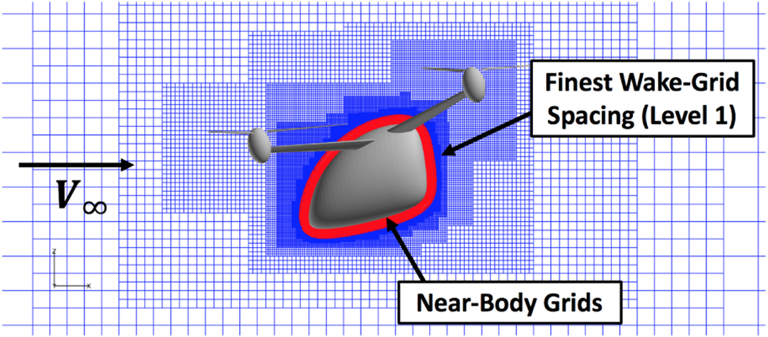
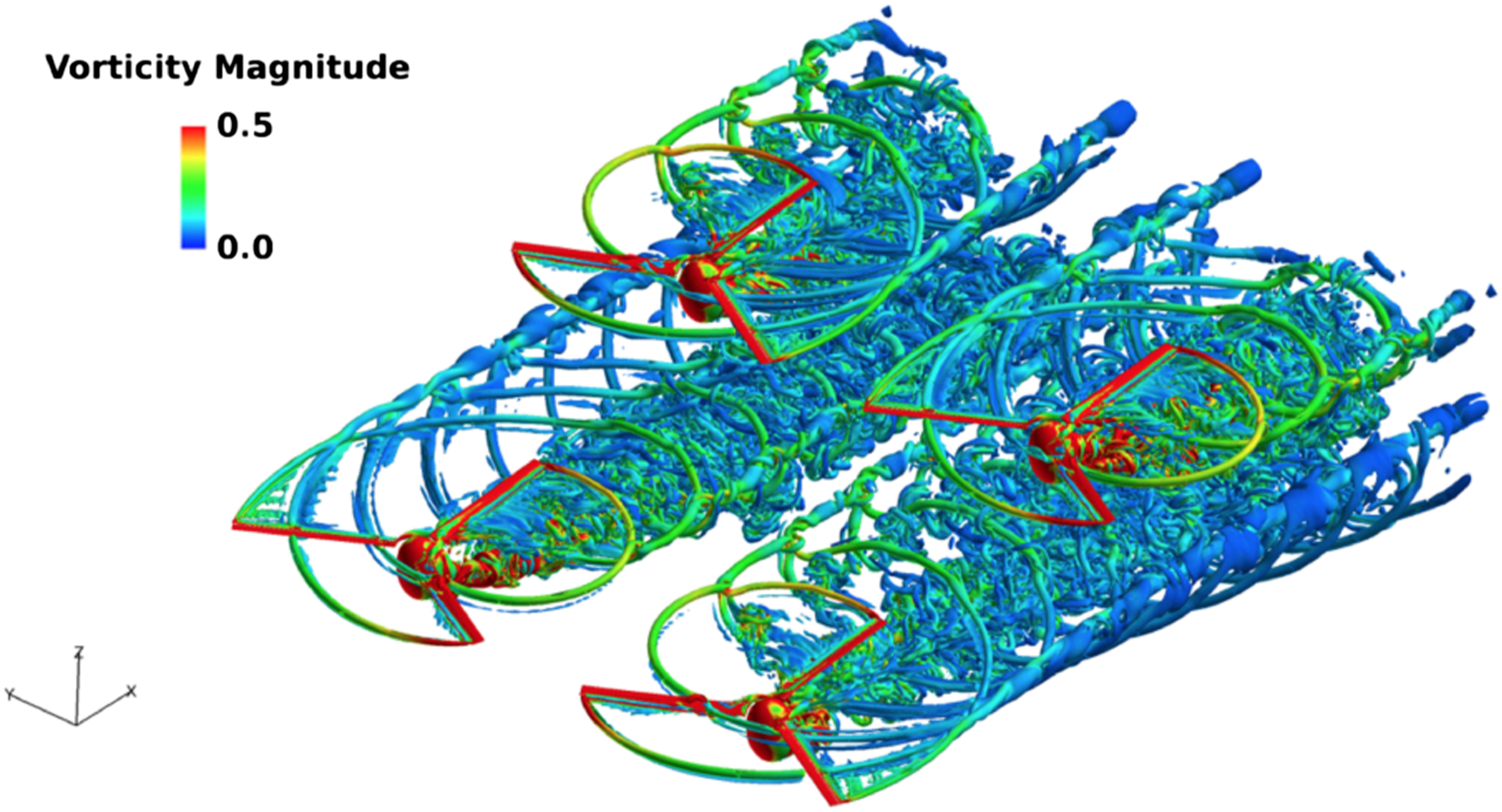
Another prediction performed by Yoon et al.
176
simulated two different small scale drones. While not acoustically focused, it provided a good visual indicator of the effects of the vehicle body on acoustics through unsteady pressure fluctuations. This experiment also used NASA’s OVERFLOW solver with Chimera grids to separate near-body and off-body simulations. Here, a fourth order accurate scheme was used in space while dual time-stepping is used for second order time integration. A DES approached based on hybrid RANS/LES is used for turbulence modeling. Figure 48 shows an unsteady surface pressure distribution that would have a significant effect on acoustics if ignored. Surface pressure distribution and q-criterion iso-surfaces of SUI Endurance quad-copter (Ref. 176).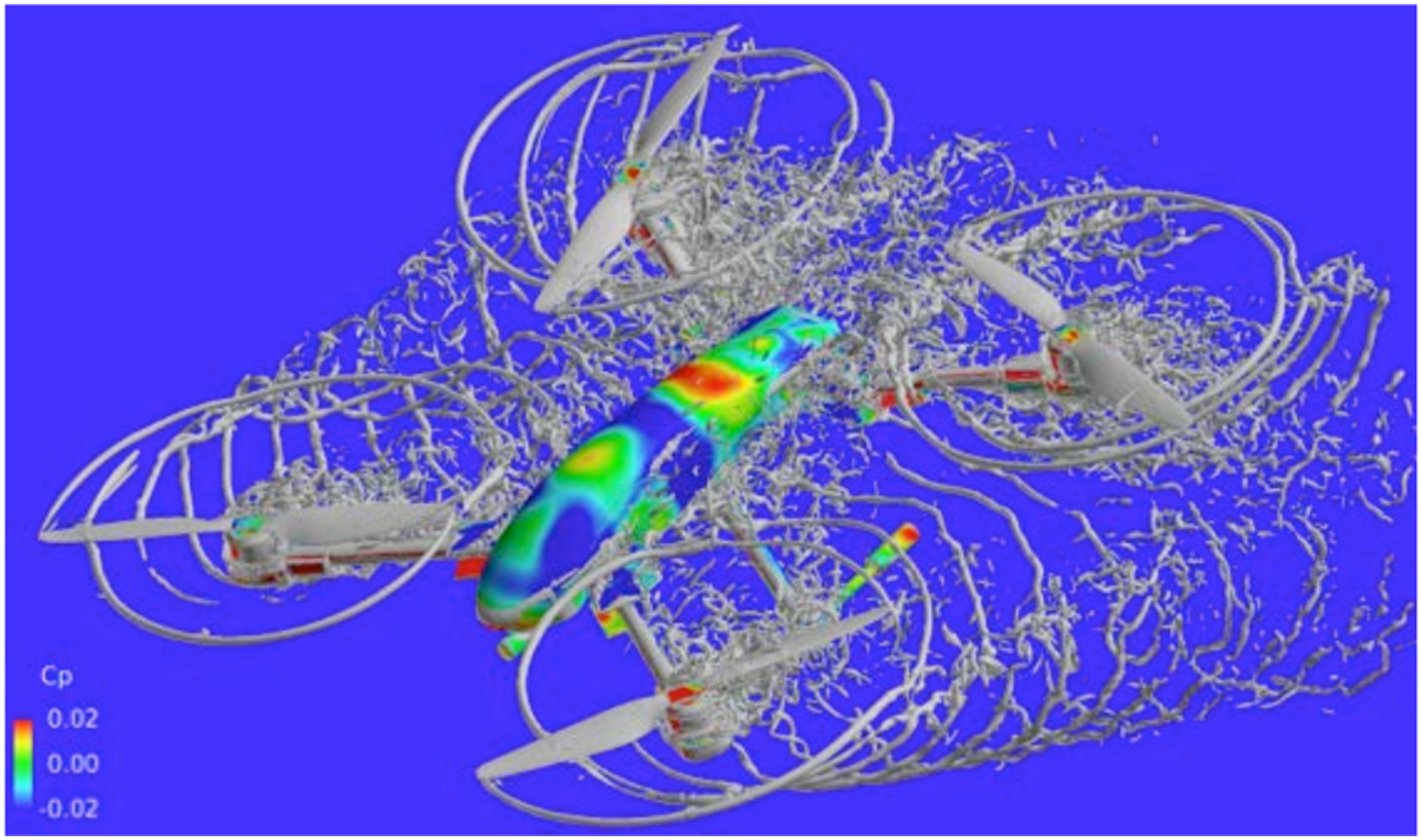
Alternative approaches
A number of alternative approaches have gained traction in recent years as well. These are methods that do not directly solve the Navier-Stokes equations (or some approximation), but rather capture the physics through different governing equations that can then be related back to state variables of interest. Specifically, the Viscous Vortex Particle Method (VVPM) and the Lattice-Boltzmann Method (LBM) have recently been used to accelerate and improve aerodynamic and acoustic predictions in the eVTOL space.
The Viscous Vortex Particle Method
is a promising alternative to Navier-Stokes CFD (NS-CFD) for simulating eVTOL wakes. Based on the vorticity transport equation, the viscous vortex particle method is a Lagrangian based method that operates on particles and has no meshes. Based on the number of particles being released from a lifting surface, the method can be considered to scale from mid-fidelity to high-fidelity by adjusting the amount of particles used in the simulation. Alvarez and Ning 177 presented a method for eVTOL aerodynamics using VVPM. They demonstrated the exceptional wake-capturing ability of the method, attributed to its lack of numerical dissipation, while being far more computationally efficient than NS-CFD. Alvarez and Ning 178 also demonstrated good qualitative agreement between particle image velocimetry measured wake geometries and those produces by their code. The inclusion of the viscosity term enables the method to simulate the turbulent breakdown a wake experiences as it ages. Alvarez et al. 179 have also compared the acoustic output with RANS computations, showing very good agreement between the methods at a much lower cost. It is important to note however, that broadband predictions were still carried out using semiempirical methods, as VVPM does not model the physics necessary to compute airfoil self-noise.
The Lattice-Boltzmann Method
is seeing expanded use in the area of high fidelity simulation. Instead of discretizing the Navier-Stokes equations, it instead discretizes the Boltzmann equation. 180 The origins of the approach date to 1988 when McNamara and Zanetti 180 discretized the Boltzmann equation using the lattice-gas automata framework. This discretization came in the form of predicting the travel of particle distributions along characteristic paths after performing a collision step at each lattice point. Although this initial approach did not have a strong physical basis, a few years later, more first principle physics would be leveraged 181 through use of a collision operator that was developed nearly 50 years prior by Bhatnagar et al. 182 This collison operator is now referred to as the BGK operator. As the name suggests, LBM simulations take place on a rectilinear lattice, thus simplifying implementation. Furthermore, setting up simulations of complex geometries can be easily automated, since there is no need for meshing. Instead, bodies can be represented by simply finding the intersection of the geometry with the characteristic directions.
At a high level, an LBM timestep consists of two steps: collision and streaming. The collision step generally involves relaxing particle distributions to an equilibrium state. Of course, in the presence of external forces or bodies, the distributions will never reach equilibrium. The streaming step then takes the collision results and propagates the distributions along characteristic vectors. The characteristic vectors represent the movement of particle distributions separated from the bulk flow. In literature, the lattice type is often referred to in a DdQq format, where d is the number of physical dimensions and q is the number of characteristic vectors; e.g. D2Q9 denotes a two dimensional lattice with nine characteristic vectors that lead to neighboring lattice points. Through a Chapman-Enskog analysis, the Navier-Stokes equations can be recovered and thus macroscopic states such as density, momentum, and pressure can be computed. 183 At its simplest, LBM is isothermal and only weakly compressible, limiting the regime of validity, but still being practically useful. The low tip-speeds of eVTOL aircraft put them comfortably in this useful regime. With the addition of additional characteristic vectors, more physics can be added to overcome these limitations, such as compressibility and thermal convection. Through all this evolution, LBM has maintained its simplicity of implementation and ease of parallelization, making it extremely well-suited for modern high performance computing hardware.
In regards to eVTOL vehicle simulation and acoustics, LBM has very favorable properties. Brès et al. 184 studied the acoustic properties of the BGK collision operator, demonstrating the low dispersion and dissipation characteristics of the method up to several kHz. There has also been work to develop collision operators specifically for acoustics. Xu and Sagaut 185 devised optimal parameters for acoustic propagation for the multiple relaxation time collision operator. Their collision operator showed not only much better dispersion and dissipation relations, it also decoupled the acoustic modes from the shear modes while enhancing the stability of the method. More recently Brogi et al. 186 developed a collision operator for acoustics that regularizes the BGK operator based on the expansion of Hermite polynomials. Their collision model remains relatively low-cost, but greatly improves the stability and accuracy of the method.
A number of computational experiments have been performed that demonstrate the strengths of LBM for aeroacoustic simulation. Casalino et al. 187 performed a proof-of-concept study using LBM coupled with FW-H equation to optimize the trajectory of an eVTOL aircraft using a noise hemisphere database approach. Using SIMULIA PowerFLOW, they computed 90 different flight cases and with each case taking between 4–8 thousand CPU hours (kCPUh). They regarded the coupling as industry-ready and noted that future work should study flight state trimming, flight dynamics/aerodynamic coupling, and optimizing hemisphere database population. Another study by Casalino et al. 188 used LBM in a proof-of-concept comprehensive CAA simulation where the noise of a hovering eVTOL aircraft was simulated and propagated across a city block. The simulation took 250kCPUh to complete on a 1000 core distributed memory machine, and consisted of 7 variable resolution regions with the coarsest resolution in the far field. In the far field, the simulation maintained 30 points per wavelength at the first blade passage frequency (BPF). They also note that the far-field resolution is sufficiently resolved to obtain qualitative information up to the third BPF.
The Lattice-Boltzmann Method has also demonstrated the ability to compute reasonably-accurate airfoil self-noise on the scale of a single rotor. Thurman et al. 167 conducted a computational study of a DJI Phantom 3 drone rotor using SIMULIA PowerFLOW. It was not a standard LBM simulation, in that turbulent wall functions were used to perform a very large eddy simulation (VLES). Their simulation used about 232kCPUh to complete, but they were able to demonstrate the broadband capabilities of LBM up to 10–20 kHz.
Full vehicle noise characterization
While measurements and predictions of isolated or interacting components are valuable for establishing the fundamental governing physics of noise generation, they are not sufficient to fully characterize the noise of electric aircraft under realistic operating conditions. As described previously, rotor and propeller noise is highly sensitive to changes in the aerodynamic operating condition. The operating conditions of the rotors and propellers are determined by the flight mechanics of the vehicle, the vehicle flight control system, pilot or operator commands, and external disturbances that may change the flight state of the vehicle. Characterizing the noise of distributed electric propulsion aircraft is further complicated by the fact that these configurations are often highly over-actuated, and can fly along the same trajectory, maneuver, or respond to disturbances in a multitude of ways.
As an example, consider the XV-15 tiltrotor aircraft shown in Figure 49, which like some electric aircraft configurations is able to tilt the rotor nacelles at different angles while maintaining the same airspeed and flight path. Acoustic flight testing of the XV-1569,189 demonstrated how noise could be controlled using this extra degree of freedom. Figure 50 shows data processed from these tests using the Rotorcraft Noise Model (RNM) Acoustic Repropagation Technique (ART)
190
to form acoustic hemispheres of A-weighted sound pressure level as a function of radiation direction for two different 70 knot indicated airspeed (KIAS) flight conditions at a −6° descending flight path angle. Azimuth angles are shown along the perimeter of the plot, with 0° and 180° azimuth angles are aligned with the aircraft tail and nose, respectively. Elevation angles are plotted radially from 0° in the horizon plane to 90° directly below the aircraft. Figure 50(a) shows the hemisphere for the XV-15 in a “helicopter” mode flight configuration, with an 80° rotor nacelle tilt angle. Noise is strongly radiated ahead of the vehicle (toward 180° azimuth) in this configuration due to the presence of strong blade–vortex interactions. In contrast, the XV-15 in “conversion” mode with a 60° rotor nacelle tilt angle, such as shown in Figure 49, radiates significantly less noise in the forward direction, since the wake convects more quickly away from the rotors. However, the noise levels do not change significantly in other directions, where other noise sources dominate. Electric aircraft configurations are often more complex, with even more excess degrees of freedom, including the ability to independently vary the RPM of individual rotors. These additional degrees of freedom offer new challenges in the characterization of the noise of these vehicles, necessitating a good understanding of the vehicle’s flight dynamics and control systems. However, understanding how flight dynamics and control affects noise generation may afford new opportunities to control and reduce the noise emissions of these new aircraft. Photograph of the XV-15 tiltrotor aircraft in conversion (NASA photo
191
). Comparison of XV-15 noise hemispheres at different nacelle tilt angles for the descending flight condition (70 KIAS and −6° degrees flight path angle).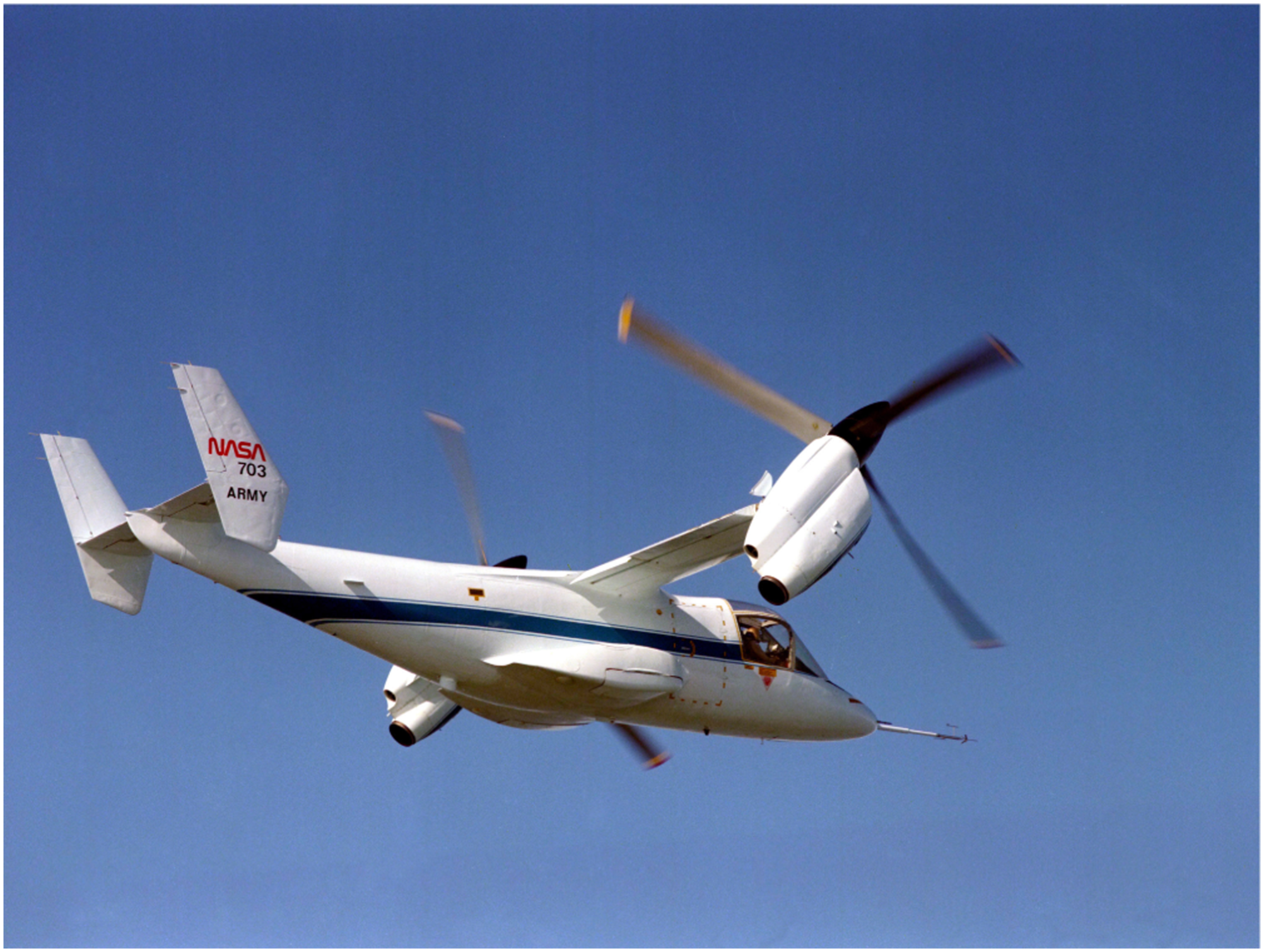
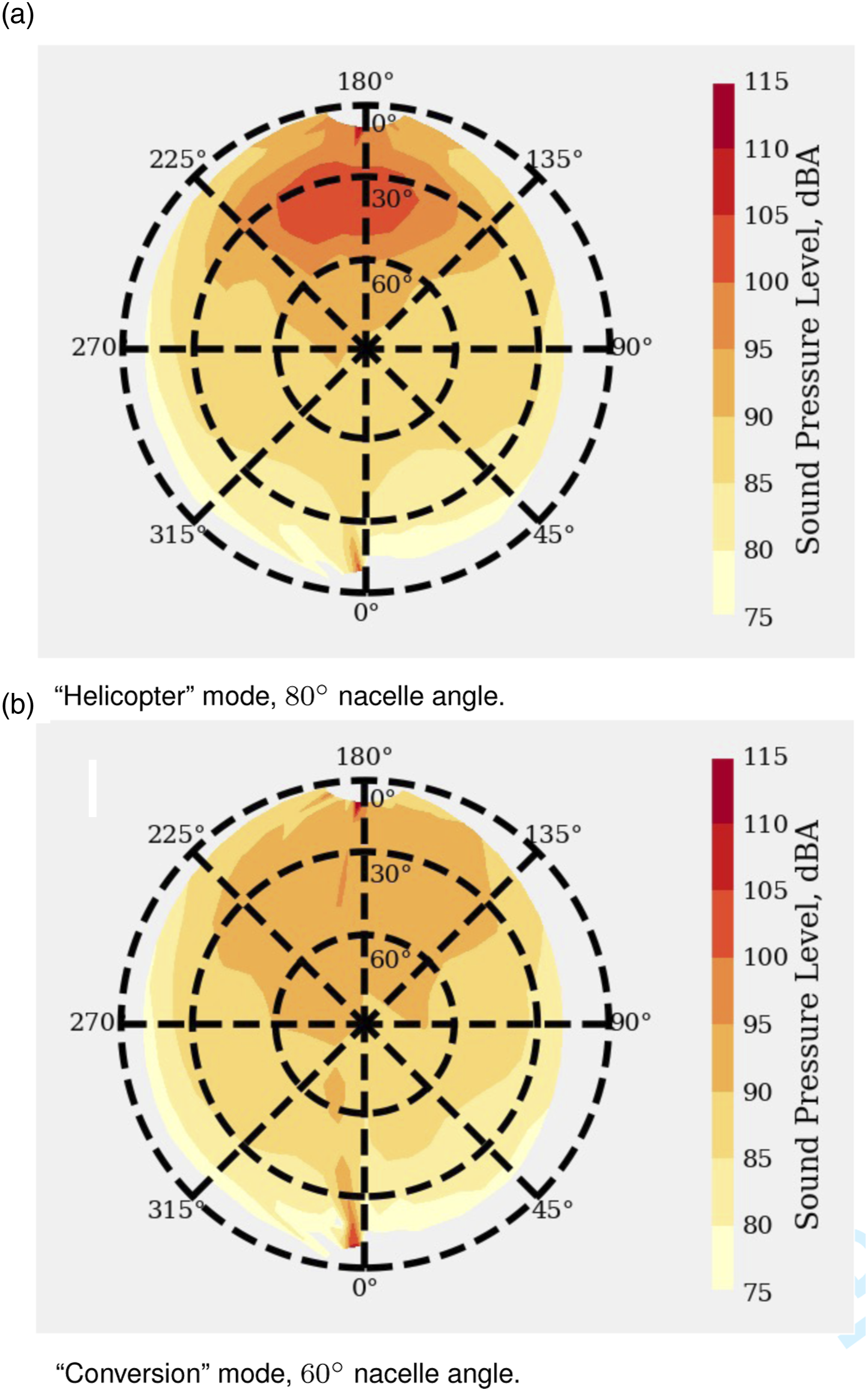
Noise prediction of full eVTOL aircraft is the focus of the Federal Aviation Administration’s (FAA) Center of Excellence for Alternative Jet Fuels and Environment (ASCENT) Project 49, work being conducted by a team that includes the authors. This project involves developing and using a noise prediction system capable of simulating arbitrary maneuvers of eVTOL aircraft, and computing the resulting noise.
192
Sample results from this noise prediction system are shown in Figure 51, for a 50 knots level turn of a generic eVTOL aircraft shown in Figure 52. This turn is flown using two different control strategies: varying rotor angular speed, and varying blade collective pitch. Across both cases, the aircraft velocity, pitch, and total rotor thrust are kept nearly-equal throughout the flight. Figure 51 demonstrates that these two control schemes generate markedly-different noise footprints, emphasizing how the overactuation of eVTOL aircraft provides opportunities for low-noise operations. Overall sound pressure level (OASPL) of Generic eVTOL aircraft (Figure 52) in 50 knots level turn, flown by varying rotor speed (top) and collective pitch (bottom); results generated by Bhaskar Mukherjee. Generic eVTOL aircraft configuration.
193
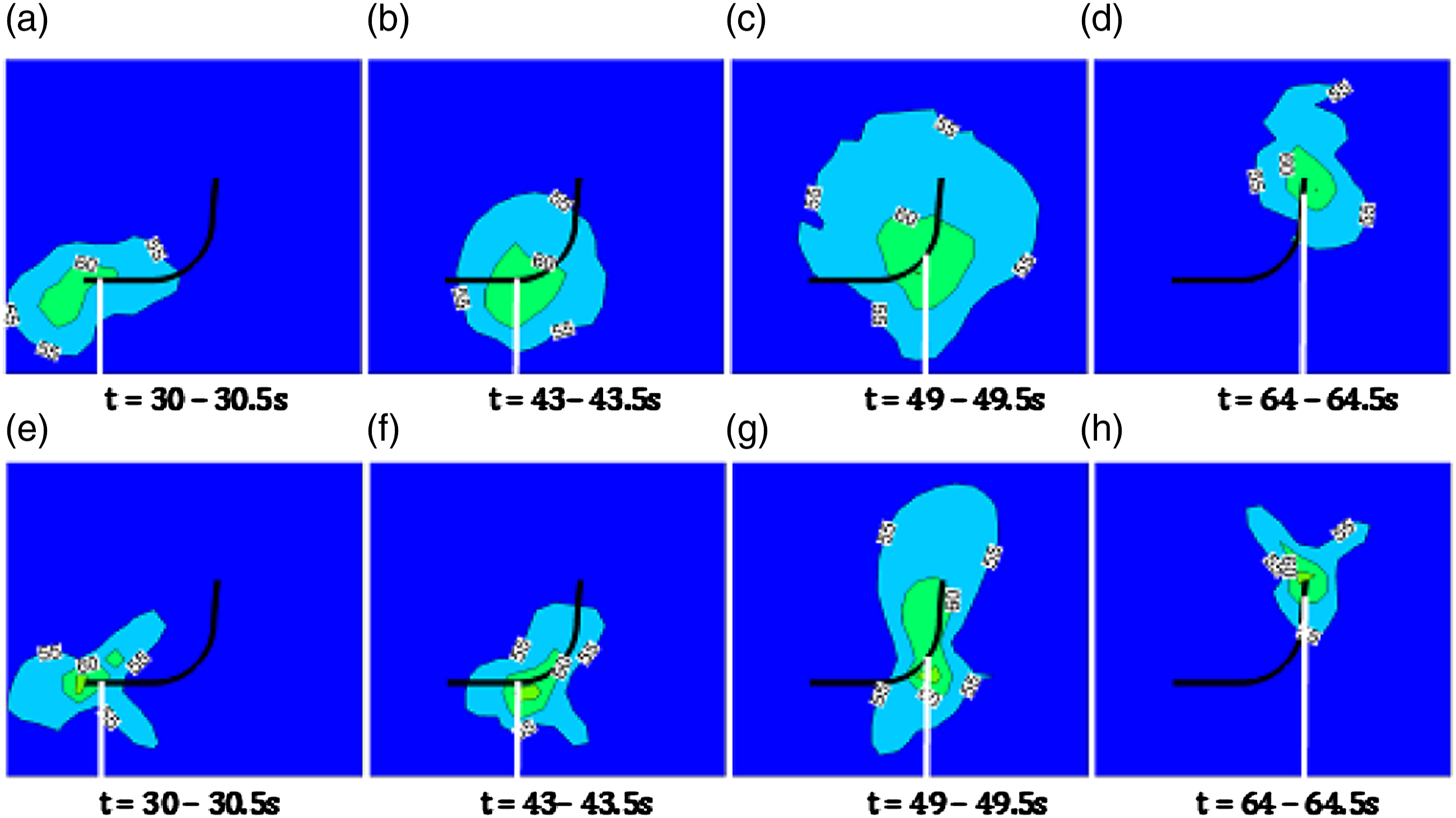
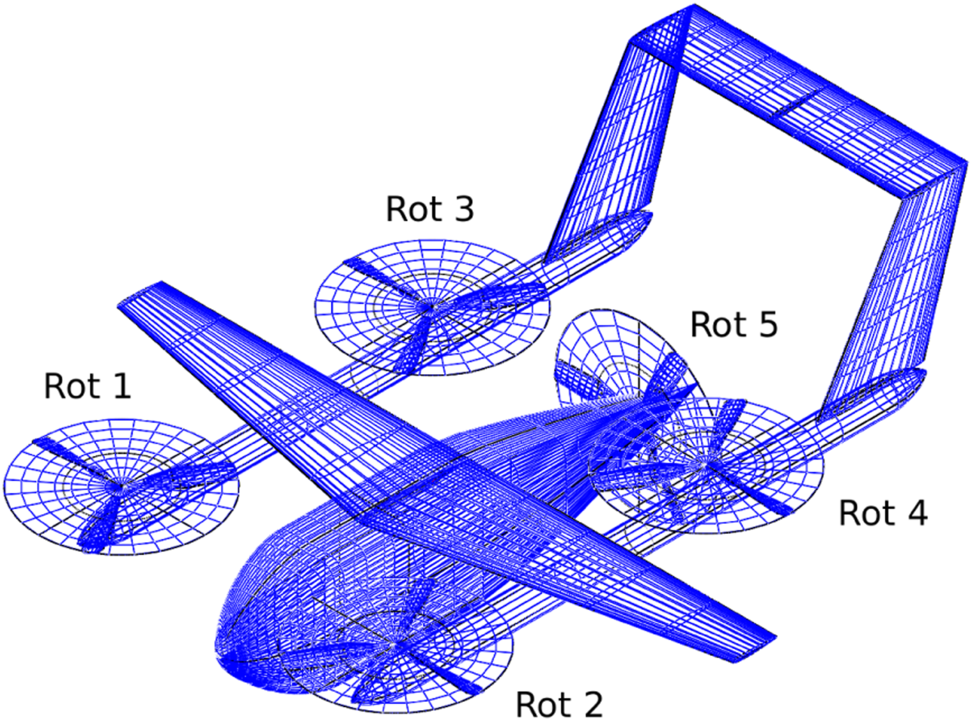
Despite the perceived challenges to predicting the full vehicle noise of eVTOL aircraft in maneuvering flight, there exist potential opportunities for simplifying the noise prediction process. For example, varying rotor speed may be a primary means of control for eVTOL aircraft, thus introducing a new problem, as most existing rotor noise analyses assume constant rotor speed (a.k.a. RPM, angular speed). 192 However, analysis conducted by the Gan et al.99,192 showed that the thickness noise of a variable RPM rotor can be considered “quasi-steady”: at any instant in time, the noise of a variable RPM rotor is nearly equal to the noise of the same rotor operating at a constant RPM equal to the instantaneous RPM of the variable RPM rotor. The main parameter governing the accuracy of this quasi-steady assumption was found to be the ratio of tangential to centripetal acceleration, which was found to be much less than one for a notional manned-scaled eVTOL aircraft.99,192 Further research is needed whether this quasi-steady assumption can be applied to simplify loading noise analysis. Another possible simplification could be to treat sources as nondeterministic or incoherent.
Pascioni, Rizzi, and Schiller demonstrated the potential of rotor phasing to reduce the noise of multi-rotor aircraft, although the phase synchronization must be accurately controlled. 194 Further evidence for this was provided in previous work by the authors, in which interference patterns in the noise directivity of multiple constant speed rotors were observed due to coherent phase relations between the rotors; in contrast, the noise of the variable speed rotors did not add coherently (Ref. 192, Figures 21 and 22). These simplifying assumptions may improve understanding of the first-order drivers of electric aircraft noise generation and can make it more feasible to model entire electric aircraft using higher fidelity tools, such as the lattice Boltzmann method described in the prior section. However, these assumptions have yet to be validated through comparison of predictions to measured acoustic and performance data for free flying electric aircraft under realistic operating conditions.
Measurement techniques for conventional propeller-driven aircraft and rotorcraft are well established. However, these techniques typically assume that the acoustic state of the vehicle does not change over the duration of a steady state pass over a microphone or microphone array. Unmanned Aircraft System (UAS) and Urban Air Mobility (UAM) platforms violate the steadiness assumption employed in the measurement and modeling of conventional aircraft noise. The rotor or propeller states, such as RPM or blade pitch angle, will vary continuously and independently as the vehicle control system responds to atmospheric perturbations. Many of these vehicles employ distributed propulsion systems, where the rotors or propellers are not locked in phase. When multiple rotors or propellers operate at similar blade passing frequencies, coherent addition of the tonal noise will result in lobes of acoustic radiation that are tightly focused in certain directions. As the phase relationships between the rotors change over time, the directionality of these lobes will vary. Consequently, the noise cannot be modeled as a single stationary source, and no two flight passes will result in the same noise radiation pattern on the ground. Moreover, because there are numerous possible combinations of control inputs that result in the same flight condition, there is no longer a unique mapping of the flight condition of the vehicle as a whole to a corresponding acoustic state.
To address these issues, the FAA has been supporting the development of measurement techniques for distributed electric propulsion vehicles through ASCENT Project 77. Under Project 77, the Pennsylvania State University is supporting the FAA in determining noise measurement and analysis methods that will allow the external noise radiation of a variety of Unmanned Aircraft System (UAS) and Urban Air Mobility (UAM) vehicles to be accurately characterized. Noise measurements are being collected for a wide range of configurations across different operating modes, flight speeds, and altitudes. Highly reconfigurable multirotor UAS have been developed for this project and will be tested in order to assess the effects of rotor number, blade design, and position on the radiated noise and the measurement and analysis process. A source separation process has also been developed, based on the Vold-Kalman order tracking filter,
195
which allows the contributions of the individual rotor or propeller noise sources to be separated and modeled independently, so that the variability in noise generation can be correlated to the variability in the vehicle flight state. Figure 53 shows the overall sound pressure level time histories for 30 individual flyover passes of a Tarot X8 octocopter at a 50 foot altitude above the microphone and nominal flight speed of 20 miles per hour
196
in both “upwind” and “downwind” directions over the microphone array. All time histories are aligned such that the vehicle was directly overhead of the microphone at 0 seconds. Depending on the observer angle, anywhere from 5 to 10 dB of variation in levels can be observed between nominally identically flight conditions, due to the high variability of the source. The sources of this variability need to be better understood if the noise of distributed electric propulsion aircraft is to be accurately and repeatably characterized. In addition to ASCENT Project 77, other researchers are working to develop measurement techniques for electric aircraft, for example through the NASA UAM Noise Working Group.
197
In 2021, NASA collaborated with Joby Aviation through the Advanced Air Mobility National Campaign to collect acoustic data for the Joby aircraft using a 50 microphone array (Figure 54), although no plans to make these data available to the public have been announced. Acoustic data such as these are needed by the research community in order to better understand how the noise of distributed electric propulsion aircraft is influenced by the flight mechanics and control systems of the vehicle under realistic operating conditions. Comparison of overall sound pressure level time histories for 30 repeated flyovers of a Tarot X8 octocopter.
196
Joby aircraft photographed next to the NASA Mobile Acoustics Facility during acoustic measurements for the 2021 Advanced Air Mobility National Campaign.
198
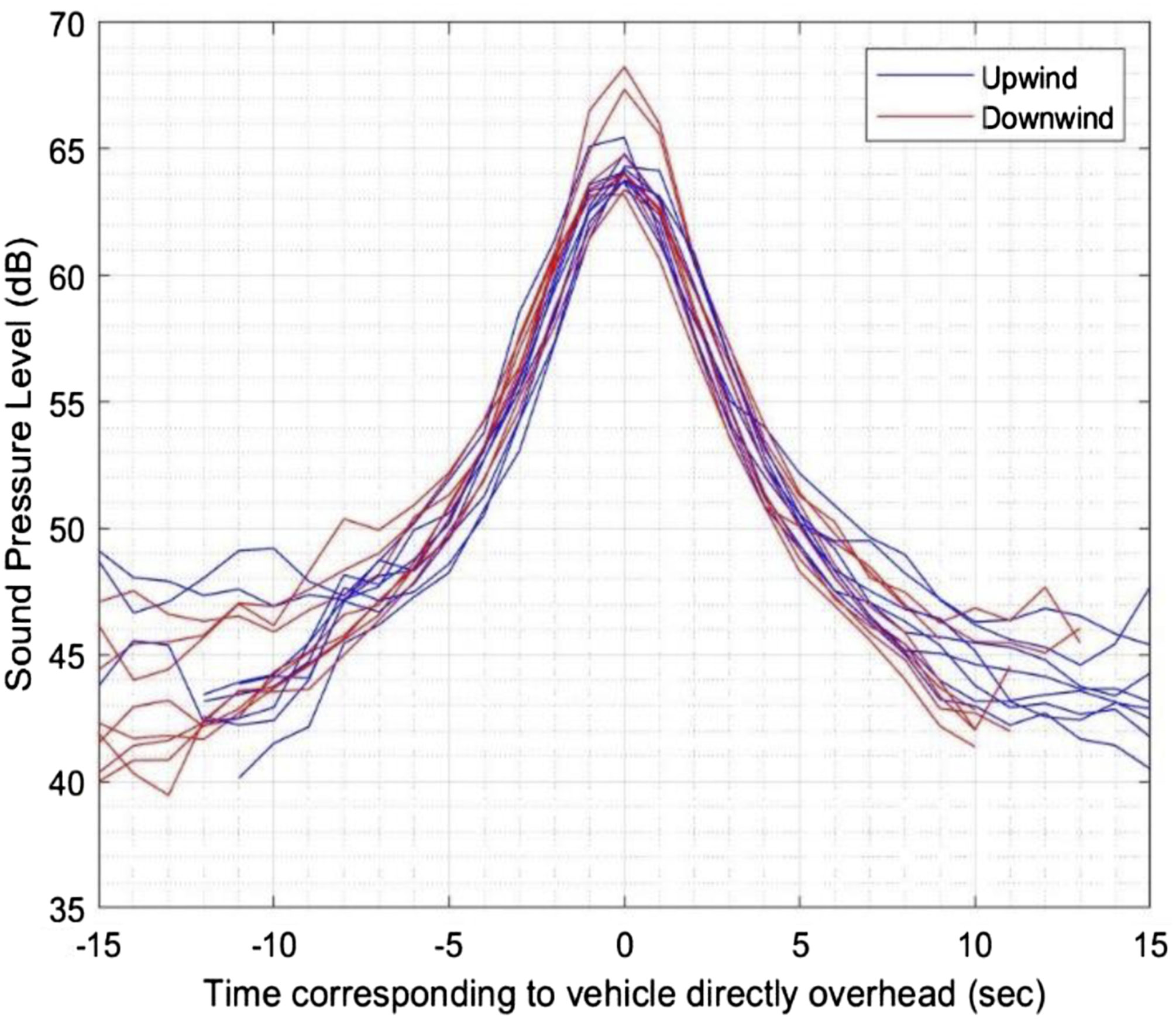
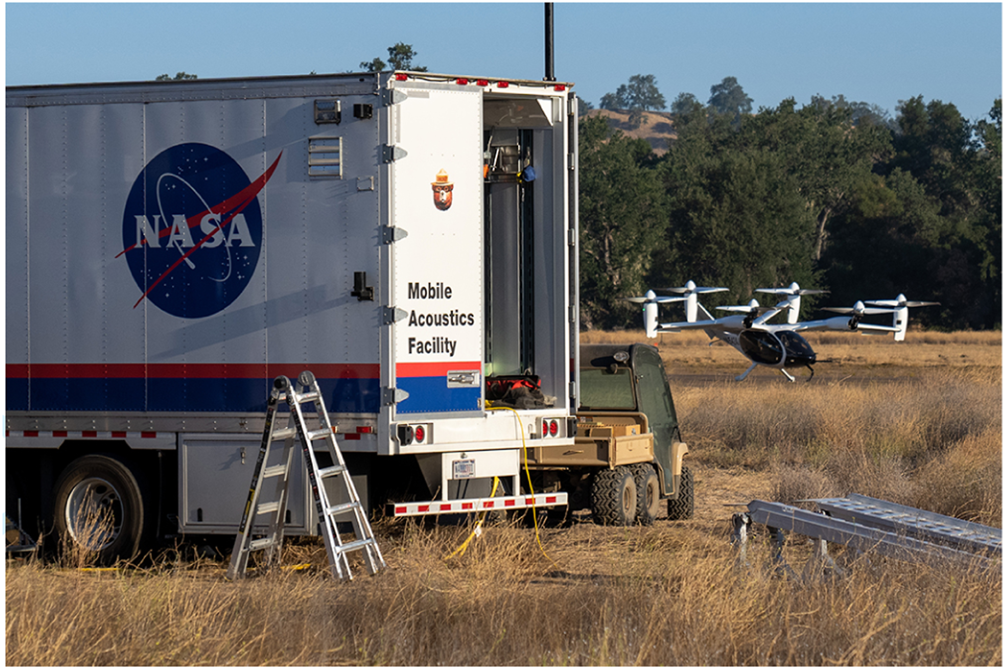
Human perception
Community acceptance of electric aircraft (especially urban operations) will likely depend heavily on the public’s response to their noise. Human perception of electric aircraft noise has been reviewed by Rizzi et al., 197 and summarized by Gan (Ref. 99, Chaps. 1.2.3 and 3.4). Rizzi emphasizes that human perception of noise must be considered throughout the design process of electric aircraft; Rizzi 199 calls this “perception-influenced design”. Perception-influenced design leverages existing knowledge on psychoacoustics, the study of human physiological and psychological responses to sound.
Central to perception-influenced design is the use of noise metrics that quantify human perception of noise, 199 beyond simply noise levels. Rizzi 199 emphasizes that aircraft noise certification does not ensure that the noise is acceptable to the public. Existing noise certification metrics generally do not fully-capture human perception of the noise of existing aircraft, let alone future electric aircraft, which may generally have different noise characteristics. Even if noise certification metrics are not updated to better-account for human perception, perception-influenced design remains important for public appeal and acceptance of electric aircraft. Psychoacoustic tests employing auralization may help determine metrics quantifying human perception as part of the perception-influenced design process.197,199,200 These tests may also promote community engagement, which may help electric aircraft and their operations obtain greater public acceptance. 197 One example of psychoacoustic testing of aircraft was conducted by Christian and Cabell, 201 who found that UAS noise was considered by test participants to be more annoying than ground vehicle noise at same noise levels. However, it remains unclear if this discrepancy is due to qualitative noise features of UAS noise. 201 Furthermore, the applicability of psychoacoustic tests of existing aircraft to electric aircraft remain unclear. 197
To date, most rotor broadband noise analyses—whether predicted or measured—have focused on time-averaged broadband noise spectra, meaning that the broadband noise sound pressure level (SPL) spectrum is integrated over a time segment on the order of a rotor period. However, in the past 3 years, the time variation of rotor broadband noise has recently increased attention202–207 due to its apparent importance to human perception of helicopter main rotor noise, as identified by Christian, Caston, and Greenwood. 106
As reviewed by Gan (Ref. 99, Chap. 1.2.1.2), rotor blade sections may experience variations in broadband noise within one rotor period. For example, edgewise flight causes variations in blade section velocity (and thus Reynolds number), which can vary the characteristics of turbulence that develops over the blade section, thus modulating self-noise. Broadband noise may also vary within a rotor revolution due to ingestion of turbulence from aerodynamic interactions or atmospheric turbulence, although this has not yet been studied extensively in the literature; to date, published studies of the time variation of broadband noise have focused on self-noise modulation in steady flight conditions without strong aerodynamic interactions. Even in hover, where the axisymmetric aerodynamic loading is steady (i.e. constant in the blade frame), broadband noise variation occurs due to the changing blade positions, convective amplification, and retarded time effects, with the latter two effects found to be especially important. 205
Li and Lee 204 quantified psychoacoustics metrics of noise modulation (fluctuation strength and roughness 208 ) for a multi-rotor eVTOL vehicle concept in steady level forward flight, demonstrating how the amplitude modulation of rotor broadband noise is reduced by increasing blade count and decreasing tip speed. The importance of time variation of broadband noise is especially-apparent for wind turbines, where noise amplitude modulation with the blade passage frequency (termed “swish”) causes greater annoyance than air and road vehicle noise at the same noise levels. 209 Other noise amplitude modulation sources (e.g. possibly caused by stall 210 ) are also reported to be especially annoying. Although most broadband noise modulation research focuses on self-noise, modulation of other broadband noise sources may also be relevant.
Psychoacoustic phenomena do not necessarily impact noise in a negative manner; there exist opportunities to leverage psychoacoustics knowledge to reduce the annoyance caused by electric aircraft noise. For example, masking could help reduce the human response to noise. 208 In general, to help achieve public acceptance, electric aircraft should not only be quiet (i.e. have low noise levels), but sound “good.” This is central to the concept of “sound quality,” 211 which has received significant interest in the automotive industry. 212
Human perception of noise is also heavily-influenced by non-acoustic factors, termed “virtual noise.”6,213 Virtual noise is not directly caused by noise levels, but triggered by noise characteristics, such as tonality, “impulsiveness” of noise, being startled by the sudden onset of noise, etc.6,213 Furthermore, noise perception of helicopters is affected by factors unrelated to noise, such as the perception of safety (e.g. fear of crashes), privacy invasion (e.g. low flyovers), and the utility of the flights. For example, people are more annoyed by helicopter taxis for the wealthy, compared to helicopter flights needed for oil drilling operations that are crucial to the local economy. 6
Virtual noise effects observed for helicopters are expected to also be important for UAM aircraft 214 : especially community perception of safety, privacy, and the utility of flights. Since UAM aircraft have unique unfamiliar appearances, this may cause them to be perceived as less proven technology and therefore less safe. Similarly, the authors speculate that aircraft appearances perceived as “inelegant” by the public may be perceived as noisy due to virtual noise: an aircraft that is subjectively deemed to look “good” (e.g. streamlined, closer to fixed-wing aircraft) will likely be perceived as “looking” safer and quieter. Virtual noise effects observed for helicopters also imply that if UAM aircraft are seen as serving merely the wealthy and not the community at large, they will receive widespread public opposition. Virtual noise effects also suggest that UAM aircraft should be designed to have distinct noise signatures from helicopters that are not easily-identifiable, to reduce the probability of triggering the same negative reactions as helicopter noise. In summary, human perception of eVTOL aircraft noise is an important area of active research that may strongly impact the public acceptance of electric aircraft operations. One major effort in this area is led by Subgroup 3 of the NASA UAM Noise Working Group. 197
Acoustically aware aircraft
Due to the high sensitivity of rotor noise to the operating state of the vehicle, noise abatement operations can be a powerful tool to reduce the noise of rotorcraft. The effectiveness of tailored noise abatement operations is well known for helicopters,215,216 where the focus has been on reducing BVI noise generated during the approach to a landing site. In addition to tailoring the trajectory to avoid flying near noise-sensitive areas, e.g. by using a steep approach to maximize the altitude above ground, noise is also reduced at the source by managing the flight condition of the vehicle. For example, BVI noise can be reduced by avoiding the rotor disk angle of attack where the strongest BVI occur, either by changing the flight path angle or by accelerating or decelerating 217 along the flight path. In addition to approach, more recent studies have also looked at developing low noise guidance for helicopters in maneuvering flight, 218 where different combinations of acceleration, descent, roll, and pitch rates can influence the noise radiated by the vehicle. For rotorcraft where the configuration can be changed in flight, such as tilt rotors, these configuration changes can also be exploited to reduce the size of the ground noise footprint. 69
To take maximum advantage of all of the opportunities to reduce noise through tailored operations, a great deal of attention has been focused on combining noise prediction tools with optimization techniques to automate the process of developing effecting noise abatement trajectories.219–223 Even when using simplified noise models, these direct trajectory optimization approaches are often computationally expensive, requiring many thousands of iterations and hours of computational time to produced low noise optimal guidance. The resulting trajectories can be quite complex and difficult for pilots to fly without guidance. Recent research has also shown that rotor noise can vary with changes in the ambient atmospheric conditions.224,225 In addition to weather, air traffic and other airspace restrictions can change over time and are likely to become even more dynamic as autonomous air traffic management systems enter service to address the new demands of small electric unmanned aircraft and air taxis. 226
To address the need for timely and specific low noise guidance, researchers have been developing several new approaches to managing aircraft noise. Taking advantage of increases in computing power and algorithms that use precomputed acoustic data,227,228 it is possible to predict the noise radiation of rotorcraft in real time.
229
These techniques can be used to give pilots and operators real time feedback about the acoustic impacts of the operation. One such example is the real-time noise display shown in Figure 55. The ground noise footprint of the vehicle at the current time of emission is shown on a moving map display, so that the operator can immediately observe how changes in the vehicle flight condition will effect people on the ground. Additional cues are provided to indicate how changes in the vehicle operating condition will effect the ground noise footprint; for example, colored noise ribbons can be added to the “tapes” displaying the current speed, acceleration, or altitude to show how changes in these variables are predicted to change the radiated noise. Despite these aides, the complexity of managing the acoustic state of the vehicle imposes a high demand on pilot workload. The noise display was coupled to a flight simulator so that user feedback could be collected from pilots. Users found the noise footprint display and guidance cues useful for learning how to fly more quietly. Although workload may be excessive for actual operations, the concept appears to have immediate utility as a training aid for low noise operations.
230
Recent developments have added the ability to review and “score” the exposure of sensitive areas to noise so that operators can develop low noise strategies for flying into their home airports or vertiports.
231
Screenshot of a real-time noise display training aid.
230
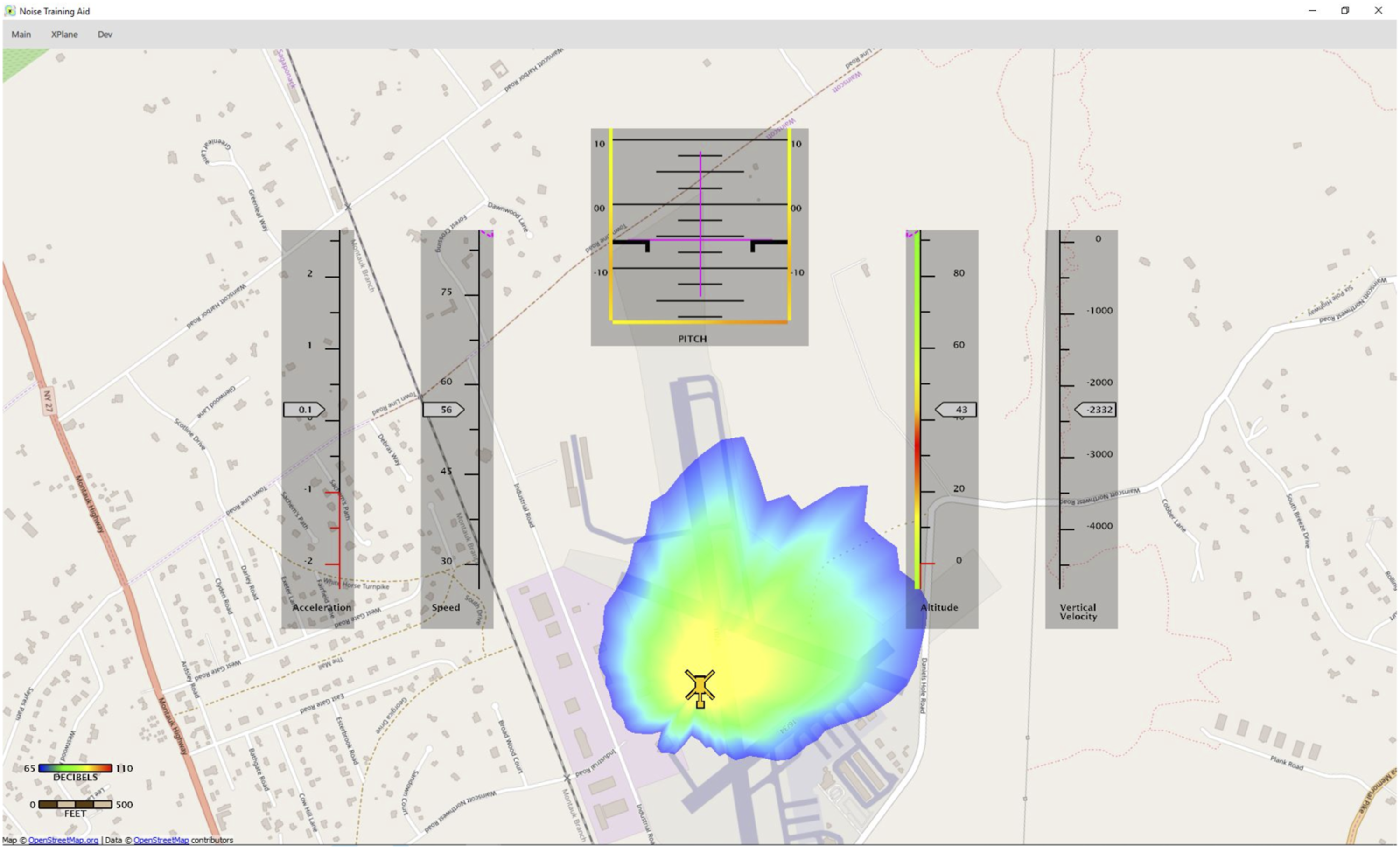
Given the rapidly increasing automation of aircraft, a better approach may be to use rapid aeroacoustic prediction to imbue aircraft with a sense of “acoustic awareness.” This would enable aircraft to manage its own acoustic state to reduce noise without burdening the pilot. Several researchers have recently investigated using optimal control approaches to rapidly determine low noise flight trajectories for rotor and propeller driven aircraft.232–234 These approaches demonstrate the feasibility of integrating acoustic awareness into vehicle flight control systems; however, it is usually necessary to use a simplified representation of the vehicle’s acoustic characteristics (e.g. as an omnidirectional source with a strength varying with tip Mach number), which may be inadequate to describe the complex mapping between vehicle flight condition and radiated noise for distributed electric propulsion aircraft. In concept, model order reduction techniques could be applied to develop surrogate models for electric aircraft noise that represent the most important acoustic trends while still being compatible with optimal control frameworks.
Another approach to the same problem takes advantage of combinatoric trajectory planning techniques that are now commonly employed in robotics. In this approach, the airspace about the vehicle is discretized into a collection of nodes, which are connected to each other with trajectories segments to form a graph. Each segment is assigned a cost associated with the predicted noise of the vehicle along that segment. Computationally efficient graph search algorithms can then be used to quickly identify the lowest cost path through the graph. Several researchers have investigated applying this approach to rotorcraft noise abatement.235–237 Figure 56 shows an example from Ref. 237 of a low noise mission plan computed between a two landing zones separated by 40 km after a section of airspace (shown in blue) is suddenly closed. The entire flight plan represents about 20 min of flight time and the low noise optimal path was computed in less than 10 s using a single CPU. This demonstrates the feasibility of “on the fly” generation of low noise guidance. However, the trajectories are still constrained by the underlying discrete structure of the graph, resulting in overly complex flight paths that are likely inefficient, difficult for pilots to track, and uncomfortable for passengers. A dynamically replanned low noise flight path around suddenly closed airspace (shown in blue).
237
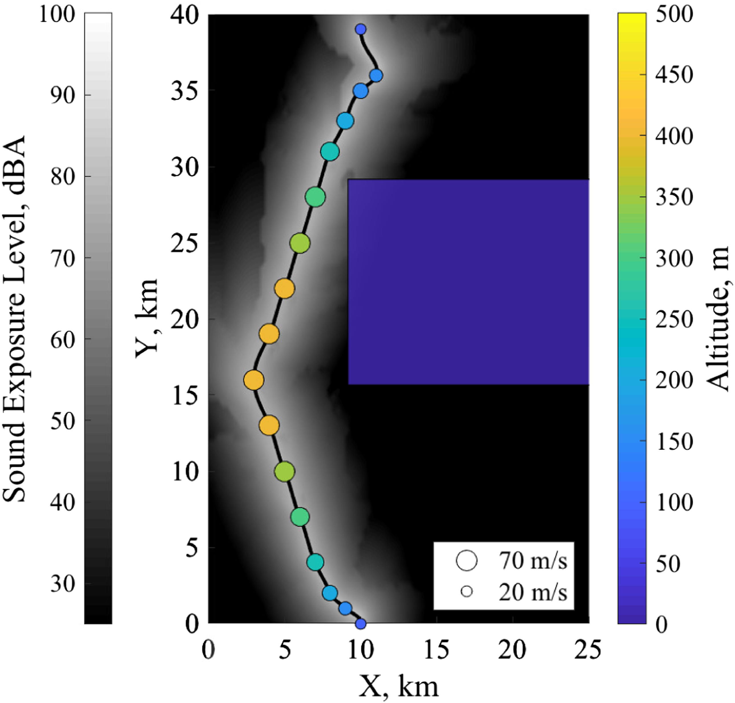
While this early work indicates that near-real-time path planning incorporating acoustic considerations is feasible, it also highlights the importance of simultaneously evaluating and optimizing aircraft operations for other practical considerations having an impact on the success of the mission. Prioritization of these parameters (e.g. noise versus energy use) may vary throughout the mission, as the operators’ awareness of the current situation develops. Furthermore, next-generation electric aircraft ranging from small drones to large transports with distributed propulsion allow the vehicle to be configured in numerous ways for a particular flight condition. Careful management of the aircraft’s state will be required throughout the operation to manage the aircraft’s performance, efficiency, and acoustic impact. While operators must be aware of these trade-offs, managing the noise of the aircraft cannot detract from their primary focus of ensuring safety of flight. Achieving an intuitive, low workload, sense of acoustic awareness will require integration of acoustic considerations into vehicle control, guidance, and flight management systems. Coordination with automated air traffic control systems may also be required to ensure that the actions of individual vehicles do not negatively impact the noise and efficiency of next generation air transportation systems as a whole. Practical realization of “acoustically aware autonomy” will require a multidisciplinary research effort including aerodynamics, acoustics, flight mechanics, control systems, systems engineering, autonomy, and human factors.
Concluding remarks
This is an exciting time in aviation, with engineers and entrepreneurs working to develop a new class of electric aircraft envisioned to operate as a new part of the urban or regional transportation infrastructure. Enabled by lightweight electric motors and distributed electric propulsion, these vehicles feature wide range of complex configurations often departing radically from those of conventional airplanes and helicopters. Since these aircraft are intended to operate frequently and in close proximity to people, achieving acceptably low noise levels is a major challenge and high priority of the burgeoning electric aircraft industry.
This is also an exciting time to be an aeroacoustician! Fundamentally, the physical mechanisms of aerodynamic noise generation for these new aircraft are not different than those of the conventional rotor and propeller driven aircraft with which we are familiar. However the low rotor tip speeds and complex flight configurations of these aircraft have elevated the importance of noise sources that have received relatively little attention for conventional aircraft. This article has sought to identify and review the body of research on the noise sources most likely to be important for electric aircraft. While the body of research on electric aircraft noise is limited—though quickly growing—inferences can be drawn from prior research on the aeroacoustics of rotors and propellers.
It is likely that unsteady loading will dominate the noise of these aircraft. The complex configurations of these vehicles raise the possibility of strong aerodynamic interactions between the components resulting in the generation of noise. While some of these interactions are relatively well understood in the research community, such as blade–vortex interaction, interactions between rotors or propellers and turbulent wakes generated by upstream aerodynamic components introduce new challenges. First principles modeling of these interactions is computationally demanding, and may be intractable for the long wake ages of interest for many electric aircraft configurations. The designers of these aircraft will need computationally efficient models of these interactions and the resulting noise to design truly quiet aircraft. To achieve this, there is a need for the research community to build a stronger physical understanding of these noise sources, building on the prior research regarding helicopter blade–wake interaction and propeller turbulence ingestion noise. Recent advances in computational aeroacoustics, including viscous vortex particle methods and the lattice Boltzmann method, will contribute to building this understanding.
Distributed electric propulsion aircraft also feature complex flight control systems, where both rotors and aerodynamic control surfaces may be used to establish a flight condition, maneuver, or respond to disturbances. The noise of the vehicle will depend on the states of the individual rotors and propellers, as well as the interactions between them. Understanding the noise generated under realistic operating conditions will require detailed knowledge of the flight dynamics and fly-by-wire control systems of these aircraft. If these interactions between flight mechanics and acoustics can be modeled accurately, it may be possible to achieve low noise aircraft operations through careful design of “acoustically aware” guidance and control systems.
Electric aircraft offer the potential for ultra-quiet aircraft operations in and around the communities they serve. Achieving this potential will require a strong multidisciplinary research effort, combining research in aerodynamics, acoustics, numerical methods, flight mechanics, autonomy, and human-machine interfaces.
Footnotes
Declaration of conflicting interests
The author(s) declared no potential conflicts of interest with respect to the research, authorship, and/or publication of this article.
Funding
The author(s) received no financial support for the research, authorship, and/or publication of this article.
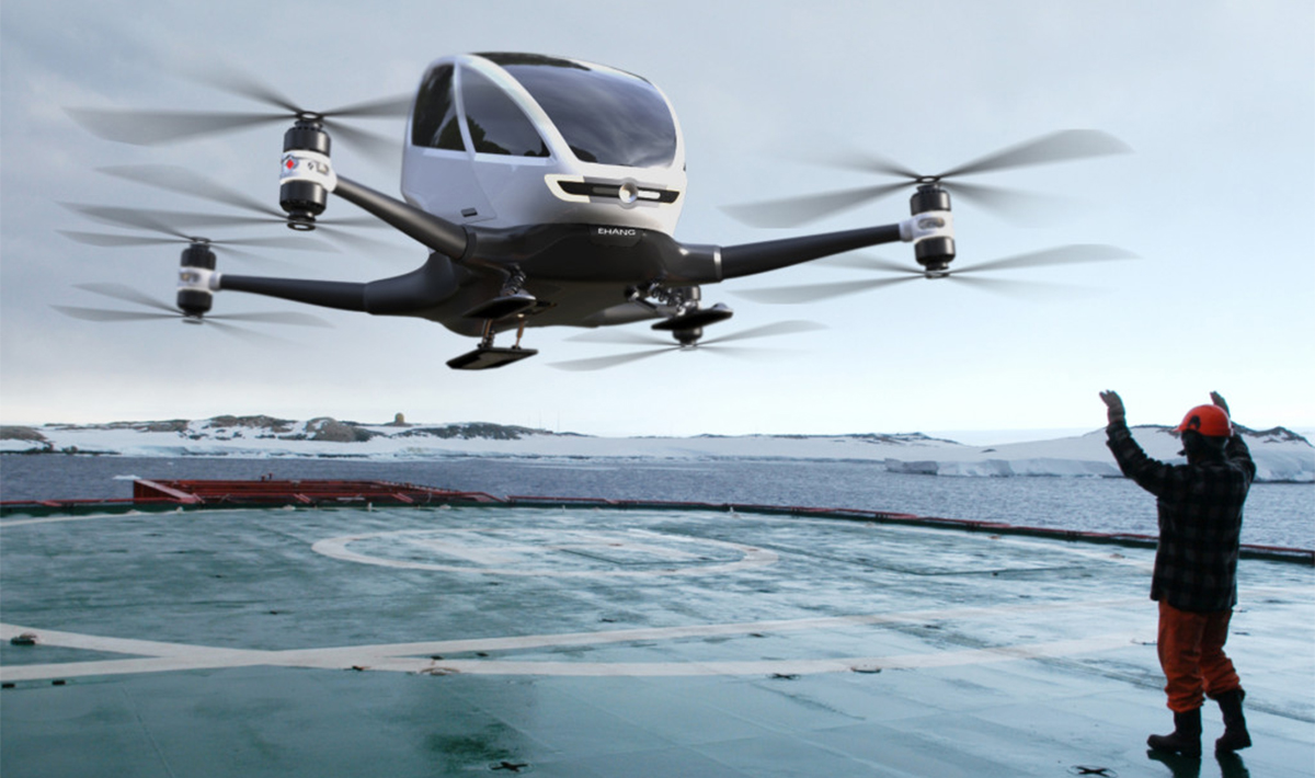
/Moog/20SureFly/Workhorse-front-flight.jpg)