Acoustic energy balances for sound radiated from duct exit with mean flow

Abstract

An old model problem for the exchange of energy between sound field and mean flow by vortex shedding has been worked out in numerical detail. The analytically exact solution of the problem of reflection, diffraction and radiation of acoustic modes in a semi-infinite annular duct with uniform subsonic mean flow, including shedding of unsteady vorticity from the duct exit, allows a precise formulation of Myers’ energy for perturbations of an inviscid mean flow. The transmitted power ${\mathcal{P}}_t$ in the duct and the radiated power ${\mathcal{P}}_f$ in the far field differ by the amounts of hydrodynamic far field powers ${\mathcal{P}}_H^i$ inside and ${\mathcal{P}}_H^o$ outside the wake (vortex sheet) emanating from the duct edge, plus the power ${\mathcal{P}}_w$ that disappears into the vortex sheet. This last component represents the source term in Myers’ energy equation. This is evidence of the non-conserved character of acoustic energy in mean flow, owing to the coupling of the acoustic field with the mean flow. ${\mathcal{P}}_f$ , ${\mathcal{P}}_H^i$ and ${\mathcal{P}}_H^o$ are always positive. This is normally the case too for ${\mathcal{P}}_w$ and ${\mathcal{P}}_t$ . But for not too high frequencies or other circumstances where shed vorticity produces more sound than was necessary for its creation, ${\mathcal{P}}_w$ and even ${\mathcal{P}}_t$ may also be negative.

Introduction

Since its formulation in the late 19th century, Kirchhoff’s expression for acoustic energy in quiescent flow ¹ has been a well-confirmed conserved quantity for the linear acoustic wave equations. During the 1960s and early 1970s several attempts were made to extend this energy as a conserved quantity to linear perturbations of inviscid flow in general.^2–5 This appeared possible for potential and homentropic flow but failed for (roughly speaking) flow with vorticity or a varying entropy. Although it was of course known from Ffowcs Williams et al^6,7or Crighton ⁸ that vorticity near sharp edges can produce sound, it was only from the experiments of Bechert^9,10 and the explanation by Howe^11,12 that it was realized that this coupling can work in the other direction too, leading to absorption of sound by vorticity. Still, it was unclear if this all plays on the level of the linear perturbations only, or that there is a coupling with the (infinite energy of the) mean flow. Only the model problem of plane waves diffracting at the trailing edge of a semi-infinite flat plate with uniform mean flow (the Sommerfeld ¹³ problem with mean flow) by Rienstra ¹⁴ yields an exact expression of the (positive or negative) acoustic energy loss into the vortical wake – present due to the unsteady Kutta condition ¹⁵ – that shows unequivocally that more energy can be “harvested” from the wake than enters from the incident waves. In other words, that there is a coupling with the mean flow.

A similar result in the form of analytic expressions for the various energy contributions was a little later obtained by Rienstra ¹⁶ for the problem of sound radiated from a semi-infinite (annular) duct with uniform mean flow, but (unfortunately) without a numerical study of its parametric dependencies.

All this was beautifully clarified and brought into a unified perspective by Myers.^17–19 He showed that the linearized energy equations (for inviscid and compressible flow with negligible heat conduction) form indeed a conserved acoustic quantity of the linearized equations if both mean flow and perturbations are irrotational and isentropic. But in the other case the energy equations have a right-hand side that can be interpreted as a source from, or sink to, the vortical perturbations or vortical mean flow, and similarly for the entropy. A remarkable side result is the fact that all this can be described without second or higher order nonlinear terms. So with the Myers equations for the acoustic energy, the energy loss to, or generation from, the vorticity in the model problems of Refs. 14 and 16 were confirmed and understood.

Unfortunately (albeit before Myers’ publications), by omitting the distinction between (a) acoustic, i.e. pressure based, energy, (b) hydrodynamic, i.e. velocity based, energy of the potential field associated to the wake, and (c) the contribution of the vortical wake itself, Howe ²⁰ drew the incorrect conclusion that our result of sound lost into or produced by the wake is wrong. Howe argued that the expression for the “acoustic dissipation” should include not only the loss into the vortical wake, but also the associated, “trapped”, hydrodynamic (but non-vortical!) field, even though this energy contribution is kinetic and not lost or dissipated at all. Of course, far from the edge the hydrodynamic field is silent and for practical purposes we could reserve the word “acoustic dissipation” to processes that reduce the audible (i.e. pressure-based) part of the acoustic energy. But this would be an ad-hoc and unphysical distinction, if there is no real dissipation but only a conversion into purely kinetic energy of convected vortices. They may be inaudible (at least, far from the edge), but there is nothing dissipated about these vortices. They could again create sound once they pass along another edge. Therefore, only when acoustic energy, including the hydrodynamic component, has been lost into the mean flow, we can say that acoustic energy has disappeared.

Extensions to the supersonic version of the problem were given by Guo ²¹ , to the scattering at a hard-wall/pressure-release-wall transition by Quinn and Howe ²² and recently to the problem of scattering by an infinite cascade by Maierhofer and Peake. ²³

Although the expression of the power lost into the wake is simple and most elegant for the plane wave, flat plate problem, the incident and radiated energy components are infinitely large and it is hard to assess how strong the effect is compared with the rest of the field. The semi-infinite duct problem is in this respect much more informative. The only problem here is that the expressions, although explicitly available and analytically exact, are more difficult to evaluate numerically because they are given in terms of complex contour integrals. Forty years ago this was a serious obstacle (while the question was not vital to the project under which the work fell), but not anymore presently. The – compared to then – superior computer equipment and numerical software we have now, make it possible to fill this lacuna. Therefore the goal of the present paper is to revisit this problem and, based on the same formulas ¹⁶ but a new numerical implementation, make a numerical study of the behavior of the various energy contributions (indicated in Figure 1 by powers = time-averaged energy fluxes across certain control surfaces) as a function of frequency, and a selection of problem parameter combinations.

Figure 1.

Sketch of configuration, with control surfaces for power integrals ${\mathcal{P}}_t$ in the duct, ${\mathcal{P}}_f$ into the acoustic far field, ${\mathcal{P}}_{\text{}H}^o$ and ${\mathcal{P}}_{\text{}H}^i$ into the hydrodynamic far field, and ${\mathcal{P}}_w={\mathcal{P}}_{\text{}w}^i-{\mathcal{P}}_{\text{}w}^o$ into the wake.

Shôn Ffowcs Williams

By this contribution I would like to honor Shôn Ffowcs Williams for his seminal and inspiring work in aeroacoustics. I remember his visits to Leen Poldervaart’s laboratory in Eindhoven ²⁴ when I was a student. His door was always open in Cambridge, and I am forever grateful he directed me to his former student David Crighton, the right person to finish successfully my PhD research.

My present contribution is a study of a model problem for sound scattering, vortex shedding, and their interaction with a mean flow. Model problems are very important for the understanding of quintessential phenomena. In a model problem they can be isolated and studied in detail, while in a full, “industrial” problem they drown in the plethora of other effects. Shôn was very keen on model problems. I remember vividly how he explained in a lecture Tyler and Sofrin’s rotor-stator interaction by a both amusing and crystal-clear comparison with the virtually backward running cartwheels of stage-coaches in old American cowboy movies.

The problem presented here is not as iconic and colorful, but I hope simple enough to add a little bit to the understanding of sound in vortical flow, and the way acoustic energy enters and leaves the mean flow.

Time-harmonic sound waves in uniform mean flow

In the next section we describe the problem and its solution as presented in ¹⁶ with a few very minor typographical simplifications. Of course, no details are given of the derivation, but inevitably the solution have to given in sufficient detail, for the meaning of the results to become clear.

The model

Anticipating the shedding of vorticity only from the trailing edge, we assume a perturbation field, irrotational almost everywhere, such that the velocity field ν may be described by a potential ϕ that is continuous except across the (after linearization cylindrical) surface formed by the trailing edge streamlines. The convective wave equation for isentropic irrotational time-harmonic (e ^iωt ) perturbations in a uniform mean flow of velocity U₀, sound speed c₀ and density ρ₀, is then given by*

$$\begin{array}{l}\mathit{v}=\nabla \varphi ,\hspace{1em}p=c_0^2\rho =-{\rho }_0\left(\text{i}\omega +U_0\frac{\partial }{\partial x}\right)\varphi \hfill \\ \left(\text{i}\omega +U_0\frac{\partial }{\partial x}\right)\rho +{\rho }_0\nabla \hspace{0.17em}\mathbf{\cdot }\hspace{0.17em}\mathit{v}=0\hfill \end{array}$$

(1)

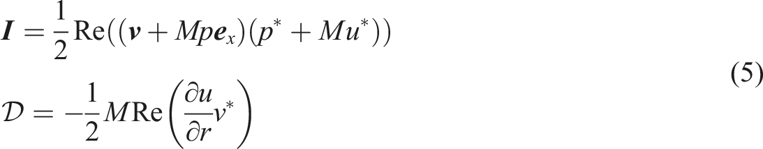
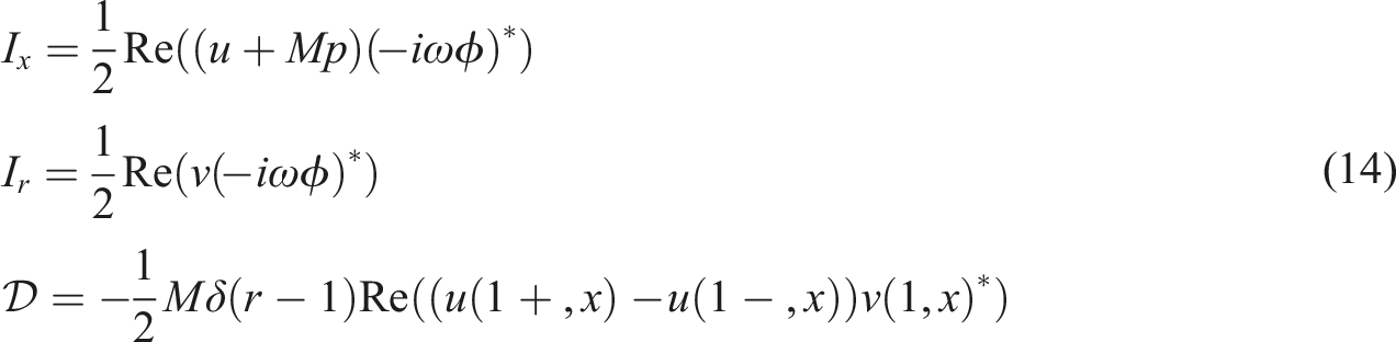
The boundary conditions are a vanishing normal velocity v along the duct walls r = h and r = a, x < 0 (Figure 1), and continuity of normal velocity v and pressure p along any trailing edge streamline r = a, x > 0. The corresponding time-averaged energy equations ¹⁹ are, for the acoustic intensity vector I (i.e. the time-averaged acoustic energy flux) and the energy source $-\mathcal{D}$ , given by

$$\nabla \hspace{0.17em}\mathbf{\cdot }\hspace{0.17em}\mathit{I}=-\mathcal{D}$$

(2)

where (neglecting viscous stress and heat conduction)

$$\begin{array}{l}\mathit{I}=\frac{1}{2}\mathrm{Re}\left(\left({\rho }_0\mathit{v}+\rho U_0{\mathit{e}}_x\right)\left(\frac{p^{\ast }}{{\rho }_0}+U_0{u}^{\ast }\right)\right)\\ \mathcal{D}=-\frac{1}{2}{\rho }_0{U}_0\mathrm{Re}\left(\frac{\partial u}{\partial r}{v}^{\ast }\right)\end{array}$$

(3)

Here, p* indicates the complex conjugate of p. As we will see, $\mathcal{D}$ can be both positive and negative, but since it is chosen with a minus sign, it is by itself a sink. Note that $\mathcal{D}$ is zero everywhere except along the vortex sheet, where $\left(\partial /\partial r\right)u\sim \delta \left(r-a\right)$ .

Non-dimensionalization

We assume the field variables and cylindrical coordinates (x, r, θ) made dimensionless: x on a, v on c₀, ρ on ρ₀, p on ${\rho }_0{c}_0^2$ , ϕ on ac₀, I on ${\rho }_0{c}_0^3$ , $\mathcal{D}$ on ${\rho }_0{c}_0^3{a}^{-1}$ . The dimensionless mean flow variables are equal to unity and will not be visible, except for the velocity, which is given by the Mach number M. All other variables will be written dimensionally and non-dimensionally the same, apart from an obvious simplification related to the θ dependence. The perturbations behave time-harmonically ∼e ^iωt with frequency ω, which is, non-dimensionally, equal to the Helmholtz number. Because of the circumferential symmetry, we may assume the field being built from Fourier θ-components and consider only one component at a time. So the perturbations will behave ∼e^{−i mθ} where integer m is also known as the azimuthal (or circumferential) modal order. All together we have the equations and boundary conditions

$$\begin{array}{l}\varphi \left(x,r,\theta ,t\right)\hspace{0.17em}\equiv \hspace{0.17em}\varphi \left(x,r\right){\text{e}}^{\mathit{i}\omega t-\mathit{i}m\theta },\hspace{1em}u=\frac{\partial \varphi }{\partial x},\hspace{1em}v=\frac{\partial \varphi }{\partial r},\hspace{1em}p=\rho \hfill \\ \left(\mathit{i}\omega +M\frac{\partial }{\partial x}\right)\rho +\left(\frac{{\partial }^2}{\partial x^2}+\frac{{\partial }^2}{\partial x^2}+\frac{1}{r}\frac{\partial }{\partial r}+1-\frac{m^2}{r^2}\right)\varphi =0,\hspace{1em}p=-\left(\mathit{i}\omega +M\frac{\partial }{\partial x}\right)\varphi \hfill \\ \{\begin{array}{ll}v\left(x,1+\right)-v\left(x,1-\right)=p\left(x,1+\right)-p\left(x,1-\right)=0\hfill & \text{if}\hspace{1em}r=1, x>0\hfill \\ v\left(x,1\pm \right)=0\hfill & \text{if}\hspace{1em}r=1, x<0\hfill \end{array}\hfill \\ v\left(x,h\right)=0\hfill \end{array}$$

(4)

and Myers’ energy expressions

$$\begin{array}{l}\mathit{I}=\frac{1}{2}\mathrm{Re}\left(\left(\mathit{v}+Mp{\mathit{e}}_x\right)\left(p^{\ast }+M{u}^{\ast }\right)\right)\\ \mathcal{D}=-\frac{1}{2}M\mathrm{Re}\left(\frac{\partial u}{\partial r}{v}^{\ast }\right)\end{array}$$

(5)

To facilitate the shedding of vorticity at the trailing edge, some form of unsteady Kutta condition, in the form of a smooth connection of the streamlines with the edge, is vital. ¹⁵ Without vortex shedding, this connection is not smooth because the pressure is singular, although the potential is continuous. This is what we usually call “no Kutta condition”. With vortex shedding, the singularity may be reduced at the expense of a discontinuous potential and (axial) velocity, i.e. a vortex sheet. This is what we could call a “partial Kutta condition”. Mathematically (at least, in the inviscid linear model), the field of the shed vorticity is an eigensolution of the problem, i.e. a solution that exists without external forcing. With the right amplitude (in other words, with the right amount of vortex shedding) this eigensolution may annihilate the singularity completely. This is the “full Kutta condition”.

Physically, vortex shedding is a process that happens for high enough Reynolds number, high enough amplitude and low enough Strouhal number. Under these circumstances the inertial forces intrinsic to the trailing edge singularity cannot be tamed by viscosity alone. In the inviscid limit that we have here, we have to select the amount of vortex shedding by an additional condition that replaces the now ineffective no-slip condition of a viscous model. Assuming the field of shed vorticity (the eigensolution of above) available from elsewhere, the extra condition will be described by a parameter γ, the amplitude of the eigensolution. This is normalized such that γ = 1 corresponds to full vortex shedding and no singularity, while γ = 0 corresponds to no vortex shedding at all. Other choices of γ are equally well possible, depending on the (viscous) problem parameters.^14,25–28

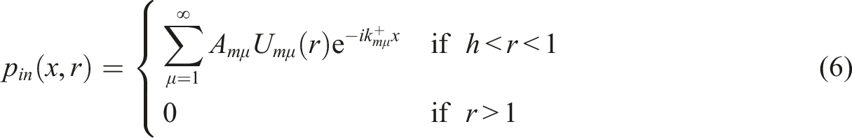
From upstream inside the duct, h < r < 1, x → −∞, an incident field p _in is assumed consisting of a sum of radial modes of amplitude A _mμ , and defined by

$$p_{in}\left(x,r\right)=\{\begin{array}{ll}{\displaystyle \sum _{\mu =1}^{\infty }{A}_{m\mu }{U}_{m\mu }}\left(r\right){\text{e}}^{-\mathit{i}{k}_{m\mu }^{+}x}\hfill & \text{if}\hspace{0.17em} h<r<1\hfill \\ 0\hfill & \text{if}\hspace{0.17em} r>1\hfill \end{array}$$

(6)

$$U_{m\mu }\left(r\right)=U_{m\mu }\left(1\right)\{\begin{array}{cc}\frac{1}{2}\pi {\alpha }_{m\mu }\left(Y_m^{\prime }\left({\alpha }_{m\mu }\right)J_m\left({\alpha }_{m\mu }r\right)-J_m^{\prime }\left({\alpha }_{m\mu }\right)Y_m\left({\alpha }_{m\mu }r\right)\right)& \text{if}\hspace{0.17em}\hspace{0.17em}h>0\hspace{0.17em}\hspace{0.17em}\&\hspace{0.17em}\hspace{0.17em}m\mu \ne 01\\ \begin{array}{l}\frac{1}{2}\pi {\alpha }_{m\mu }{Y}_m^{\prime }\left({\alpha }_{m\mu }\right)J_m\left({\alpha }_{m\mu }r\right)\\ 1\end{array}& \begin{array}{l}\text{if}\hspace{0.17em}\hspace{0.17em}h=0\hspace{0.17em}\hspace{0.17em}\&\hspace{0.17em}\hspace{0.17em}m\mu \ne 01\\ \text{if}\hspace{0.17em}\hspace{0.17em}m\mu =01\end{array}\end{array}$$

$$\begin{array}{l}{\displaystyle {\int }_h^1{U}_{m\mu }}\left(r\right)U_{m\nu }\left(r\right)r\hspace{0.17em}\text{d}r={\delta }_{\mu \nu },\hspace{0.17em}{U}_{m\mu }^{\prime }\left(1\right)=U_{m\mu }^{\prime }\left(h\right)=0\\ k_{m\mu }^{\pm }=\frac{\pm {\mathrm{\Omega }}_{m\mu }-\omega M}{{\beta }^2},\hspace{1em}{\mathrm{\Omega }}_{m\mu }={\left({\omega }^2-{\beta }^2{\alpha }_{m\mu }^2\right)}^{1/2},\hspace{1em}\mathrm{Im}{\mathrm{\Omega }}_{m\mu }\hspace{0.17em}\mathrm{⩽}\hspace{0.17em}0,\hspace{1em}\beta ={\left(1-M^2\right)}^{1/2}\end{array}$$

with a corresponding ϕ _in (x, r), and a slight exception if mμ = 01. Reference amplitude U _mμ (1) follows from the normalization. The duct hard walls require the conditions $U_{m\mu }^{\prime }\left(1\right)=U_{m\mu }^{\prime }\left(h\right)=0$ , the second of which yields the set of real α _mμ . These are all taken positive, except α₀₁ which is zero.

Solution

By introducing a Prandtl-Glauert/Lorentz transformation, complemented (for later use) by Strouhal number S and a form of spherical coordinates (R, ξ)

$$\begin{array}{l}{k}_{m\mu }^{\pm }=\omega {\overline{k}}_{m\mu }^{\pm },\hspace{1em}{\mathrm{\Omega }}_{m\mu }=\omega {\overline{\mathrm{\Omega }}}_{m\mu },\hspace{1em}{\overline{\mathrm{\Omega }}}_{m\mu }={\left(1-\frac{{\alpha }_{m\mu }^2}{{\kappa }^2}\right)}^{1/2}\\ \omega =\beta \kappa ,\hspace{1em}x=\beta X,\hspace{1em}X=R\cos \xi ,\hspace{1em}r=R\sin \xi ,\hspace{1em}S=\frac{\omega }{M}\end{array}$$

(7)

the solution can be written in the form of a Fourier transform in spatial coordinate x

$$\begin{array}{l}\varphi ={\varphi }_{in}-\frac{\kappa }{\beta }\hspace{0.17em}{\text{e}}^{\mathit{i}\kappa MX}{\displaystyle \sum _{\mu =1}^{\infty }{A}_{m\mu }}{F}_0\frac{1}{2\pi }{\displaystyle {\int }_{-\infty -0\mathit{i}}^{\infty +0\mathit{i}}{v}_{+}^2}\left(\tau \right){\tilde{K}}_{+}\left(\tau \right)\left[\frac{1}{\tau -{\overline{\mathrm{\Omega }}}_{m\mu }}-\frac{\gamma }{\tau -M^{-1}}\right]\frac{\chi }{\text{i}\kappa v}{\text{e}}^{-\mathit{i}\kappa \tau X}\text{d}\tau \end{array}$$

(8)

$$\begin{array}{l}\chi =\{\begin{array}{ll}\frac{K_m^{\prime }\left(\mathit{i}\kappa vh\right)I_m\left(\mathit{i}\kappa vr\right)-I_m^{\prime }\left(\mathit{i}\kappa vh\right)K_m\left(\mathit{i}\kappa vr\right)}{K_m^{\prime }\left(\mathit{i}\kappa vh\right)I_m^{\prime }\left(\mathit{i}\kappa v\right)-I_m^{\prime }\left(\mathit{i}\kappa vh\right)K_m^{\prime }\left(\mathit{i}\kappa v\right)}\hfill & \text{if}\hspace{1em}h>0,\hspace{0.17em}r<1\hfill \\ \frac{I_m\left(\mathit{i}\kappa vr\right)}{I_m^{\prime }\left(\mathit{i}\kappa v\right)}\hfill & \text{if}\hspace{1em}h=0,\hspace{0.17em}r<1\hfill \\ \frac{K_m\left(\mathit{i}\kappa vr\right)}{K_m^{\prime }\left(\mathit{i}\kappa v\right)}\hfill & \text{if}\hspace{1em}r>1\hfill \end{array}\\ F_0=\frac{1}{2}{\beta }^2{U}_{m\mu }\left(1\right)\frac{1+{\overline{\mathrm{\Omega }}}_{m\mu }}{1-M{\overline{\mathrm{\Omega }}}_{m\mu }}{\tilde{K}}_{-}\left({\overline{\mathrm{\Omega }}}_{m\mu }\right)\\ \tilde{K}\left(\tau \right)=L\left(\kappa v\left(\tau \right)\right)={\tilde{K}}_{+}\left(\tau \right){\tilde{K}}_{-}\left(\tau \right),\\ L\left(z\right)=\{\begin{array}{ll}\pi \frac{H_m^{\left(2\right)\prime }\left(z\right)}{H_m^{\left(2\right)\prime }\left(zh\right)}\left(J_m^{\prime }\left(zh\right)Y_m^{\prime }\left(z\right)-Y_m^{\prime }\left(zh\right)J_m^{\prime }\left(z\right)\right),\hfill & \text{if}\hspace{1em}h>0\hfill \\ -\pi i{H}_m^{\left(2\right)\prime }\left(z\right)J_m^{\prime }\left(z\right),\hfill & \text{if}\hspace{1em}h=0\hfill \end{array}\\ v\left(\tau \right)={\left(1-{\tau }^2\right)}^{1/2}=v_{+}\left(\tau \right)v_{-}\left(\tau \right),\hspace{1em}{v}_{+}\left(\tau \right)={\left(1-\tau \right)}^{1/2},\hspace{1em}{v}_{-}\left(\tau \right)={\left(1+\tau \right)}^{1/2}\end{array}$$

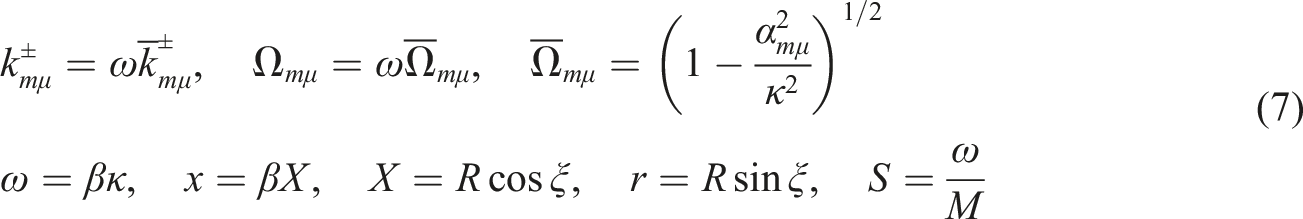
See for details Ref.16. Except for a few minor exceptions, like ω for k and the introduction of κ and S, all notations have been retained exactly the same. $J_m,Y_m,H_m^{\left(2\right)}$ denote ordinary Bessel functions and K _m , I _m modified Bessel functions. The square roots v₊ and v₋ are defined by their principal values. (Note that square root v(τ) has no relation whatsoever with the radial component of the velocity. In retrospect, it would have been wiser to choose another letter.)

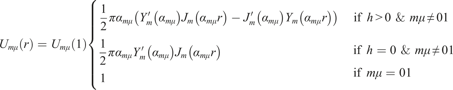
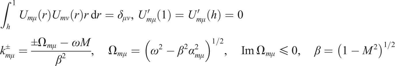
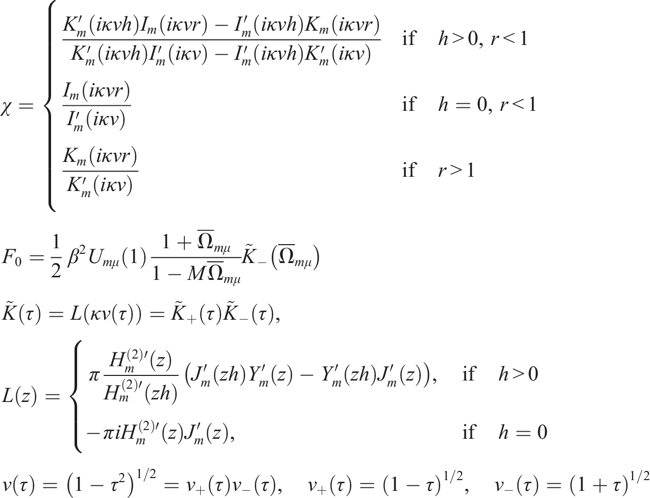
The functions ${\tilde{K}}_{+}$ and v₊ are constructed such that they are analytic in the upper complex half plane, while similarly ${\tilde{K}}_{-}$ and v₋ are analytic in the lower complex half plane. Define ^#

$$\begin{array}{l}{ℂ}^{-}=\left\{z\in ℂ\hspace{0.17em}|\hspace{0.17em}\mathrm{Im}\left(z\right)<0\hspace{0.17em}\vee \hspace{0.17em}\left(\mathrm{Im}\left(z\right)=0\hspace{0.17em}\&\hspace{0.17em}\mathrm{Re}\left(z\right)>0\right)\right\}\\ {ℂ}^{+}=\left\{z\in ℂ\hspace{0.17em}|\hspace{0.17em}\mathrm{Im}\left(z\right)>0\hspace{0.17em}\vee \hspace{0.17em}\left(\mathrm{Im}\left(z\right)=0\hspace{0.17em}\&\hspace{0.17em}\mathrm{Re}\left(z\right)<0\right)\right\}\end{array}$$

If $t\in {ℂ}^{-}$ , below the integration contour, then

$$\log {\tilde{K}}_{-}\left(t\right)=\frac{\mathit{it}}{\pi }{\displaystyle {\int }_0^{\infty }\frac{\log \tilde{K}\left(\tau \right)}{{\tau }^2-t^2}}\text{d}\tau =\mathcal{J},\hspace{1em}{\tilde{K}}_{+}\left(t\right)=\frac{\tilde{K}\left(t\right)}{{\tilde{K}}_{-}\left(t\right)}$$

(9a)

$$\frac{{\tilde{K}}_{-}^{\prime }\left(t\right)}{{\tilde{K}}_{-}\left(t\right)}=\frac{\mathit{i}}{\pi }{\displaystyle {\int }_0^{\infty }\frac{{\tau }^2+t^2}{{\left({\tau }^2-t^2\right)}^2}}\log \tilde{K}\left(\tau \right)\text{d}\tau =\mathrm{ℒ},\hspace{1em}\frac{{\tilde{K}}_{+}^{\prime }\left(t\right)}{{\tilde{K}}_{+}\left(t\right)}=\frac{{\tilde{K}}^{\prime }\left(t\right)}{\tilde{K}\left(t\right)}-\mathrm{ℒ}$$

(9b)

If $t\in {ℂ}^{+}$ , above the integration contour, then

$$\log {\tilde{K}}_{+}\left(t\right)=\frac{-\mathit{it}}{\pi }{\displaystyle {\int }_0^{\infty }\frac{\log \tilde{K}\left(\tau \right)}{{\tau }^2-t^2}}\text{d}\tau =-\mathcal{J},\hspace{1em}{\tilde{K}}_{-}\left(t\right)=\frac{\tilde{K}\left(t\right)}{{\tilde{K}}_{+}\left(t\right)}$$

(9c)

$$\frac{{\tilde{K}}_{+}^{\prime }\left(t\right)}{{\tilde{K}}_{+}\left(t\right)}=\frac{-\mathit{i}}{\pi }{\displaystyle {\int }_0^{\infty }\frac{{\tau }^2+t^2}{{\left({\tau }^2-t^2\right)}^2}}\log \tilde{K}\left(\tau \right)\text{d}\tau =-\mathrm{ℒ},\hspace{1em}\frac{{\tilde{K}}_{-}^{\prime }\left(t\right)}{{\tilde{K}}_{-}\left(t\right)}=\frac{{\tilde{K}}^{\prime }\left(t\right)}{\tilde{K}\left(t\right)}+\mathrm{ℒ}$$

(9d)

Numerical evaluation of these complex integrals are crucial for the final solution, and should be done with care. Analyticity of the integrand, however, makes it possible to avoid impeding singularities by contour deformation. See further below.

The underlying Wiener-Hopf technique is indebted to the classic solution by Levine and Schwinger ²⁹ of the problem for m = 0 and no flow and no hub. The generalizations for general m and a hub are not fundamentally different. The generalization to a uniform flow we need here, can be obtained by utilizing a Prandtl-Glauert or (which is here equivalent) Lorentz transformation to the no-flow solution, but this is not entirely straightforward. Due to the possible complication of vortex shedding in the case of an out-flow duct the singularity at the duct edge may be different without violating the edge condition. ³⁰ Therefore, we applied in Rienstra ¹⁶ the transformation along with the Wiener-Hopf procedure and relaxed the central argument of a bounded entire and therefore constant function being zero (as it tends to zero at infinity) to possibly being non-zero. We can, however, construct in a slightly more efficient way the full solution also by elementary operations on the no-flow solution, as is shown in the Appendix.

The celebrated generalization by Munt^31,32 to a jet-type mean flow (different inside and outside the duct and its extension) involves a particular difficulty that we don’t have here, namely the Kelvin-Helmholtz instability of the jet. This instability is excited by the shed vorticity (and therefore absent in case of γ = 0), but with vortex shedding it is there and its exponential growth prevents a regular Fourier transform in x. There are various ways to overcome this difficulty. Munt followed originally the approach of Jones and Morgan ³³ by introducing the Fourier transform of exponential functions as a form of generalized functions (more specifically, ultra-distributions). This is very ingenious, but only necessary in time domain. For a single frequency we can split off the exponential part and write the bounded part of the solution as a regular Fourier transform. ³⁴

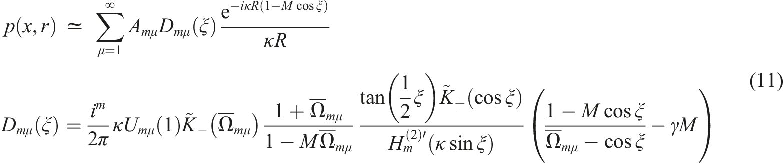
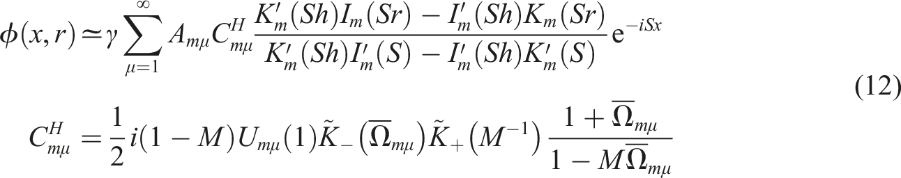
The solution made explicit in various parts of the field

The foregoing Fourier integral solution can be made more explicit in certain parts of the field. We have:

For x < 0, h < r < 1

$$\begin{array}{l}p\left(x,r\right)={\displaystyle \sum _{\mu =1}^{\infty }{A}_{m\mu }{U}_{m\mu }\left(r\right)}{\text{e}}^{-\mathit{i}{k}_{m\mu }^{+}x}+{\displaystyle \sum _{\nu =1}^{\infty }{B}_{m\nu }}{U}_{m\nu }\left(r\right){\text{e}}^{-\mathit{i}{k}_{m\nu }^{-}x}\\ B_{m\nu }={\displaystyle \sum _{\mu =1}^{\infty }{A}_{m\mu }{R}_{m\mu \nu }}\\ R_{m\mu \nu }=-\frac{1}{4}{U}_{m\mu }\left(1\right)U_{m\nu }\left(1\right)\frac{\left(1+{\overline{\mathrm{\Omega }}}_{m\mu }\right)\left(1+{\overline{\mathrm{\Omega }}}_{m\nu }\right)}{\left(1-M{\overline{\mathrm{\Omega }}}_{m\mu }\right){\overline{\mathrm{\Omega }}}_{m\nu }}\left(\frac{1+M{\overline{\mathrm{\Omega }}}_{m\nu }}{{\overline{\mathrm{\Omega }}}_{m\mu }+{\overline{\mathrm{\Omega }}}_{m\nu }}-\gamma M\right){\tilde{K}}_{-}\left({\overline{\mathrm{\Omega }}}_{m\mu }\right){\tilde{K}}_{-}\left({\overline{\mathrm{\Omega }}}_{m\nu }\right)\end{array}$$

(10)

For κR → ∞, ξ > 0

$$\begin{array}{l}p\left(x,r\right)\simeq {\displaystyle \sum _{\mu =1}^{\infty }{A}_{m\mu }}{D}_{m\mu }\left(\xi \right)\frac{{\text{e}}^{-\mathit{i}\kappa R\left(1-M\cos \xi \right)}}{\kappa R}\\ D_{m\mu }\left(\xi \right)=\frac{{\mathit{i}}^m}{2\pi }\kappa U_{m\mu }\left(1\right){\tilde{K}}_{-}\left({\overline{\mathrm{\Omega }}}_{m\mu }\right)\frac{1+{\overline{\mathrm{\Omega }}}_{m\mu }}{1-M{\overline{\mathrm{\Omega }}}_{m\mu }}\frac{\tan \left(\frac{1}{2}\xi \right){\tilde{K}}_{+}\left(\cos \xi \right)}{H_m^{\left(2\right)\prime }\left(\kappa \sin \xi \right)}\left(\frac{1-M\cos \xi }{{\overline{\mathrm{\Omega }}}_{m\mu }-\cos \xi }-\gamma M\right)\end{array}$$

(11)

For Sx → ∞, h < r < 1

$$\begin{array}{l}\varphi \left(x,r\right)\simeq \gamma {\displaystyle \sum _{\mu =1}^{\infty }{A}_{m\mu }}{C}_{m\mu }^H\frac{K_m^{\prime }\left(Sh\right)I_m\left(Sr\right)-I_m^{\prime }\left(Sh\right)K_m\left(Sr\right)}{K_m^{\prime }\left(Sh\right)I_m^{\prime }\left(S\right)-I_m^{\prime }\left(Sh\right)K_m^{\prime }\left(S\right)}\hspace{0.17em}{\text{e}}^{-\mathit{i}Sx}\\ C_{m\mu }^H=\frac{1}{2}\mathit{i}\left(1-M\right)U_{m\mu }\left(1\right){\tilde{K}}_{-}\left({\overline{\mathrm{\Omega }}}_{m\mu }\right){\tilde{K}}_{+}\left(M^{-1}\right)\frac{1+{\overline{\mathrm{\Omega }}}_{m\mu }}{1-M{\overline{\mathrm{\Omega }}}_{m\mu }}\end{array}$$

(12)

For Sx → ∞, r > 1

$$\varphi \left(x,r\right)\simeq \gamma {\displaystyle \sum _{\mu =1}^{\infty }{A}_{m\mu }}{C}_{m\mu }^H\frac{K_m\left(Sr\right)}{K_m^{\prime }\left(S\right)}\hspace{0.17em}{\text{e}}^{-iSx}$$

(13)

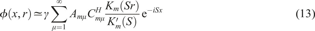
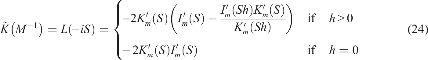
The argument M⁻¹ of ${\tilde{K}}_{\pm }$ , and (later) their derivatives, is a complex-valued point, located below the integration contour but just above the branch cut [1, ∞).

Power integrals

By using the axial component I _x and radial component I _r of the intensity vector I , and (as a check) the energy source term $\mathcal{D}$

$$\begin{array}{l}{I}_x=\frac{1}{2}\mathrm{Re}\left(\left(u+Mp\right){\left(-\mathit{i}\omega \varphi \right)}^{\ast }\right)\\ I_r=\frac{1}{2}\mathrm{Re}\left(v{\left(-\mathit{i}\omega \varphi \right)}^{\ast }\right)\\ \mathcal{D}=-\frac{1}{2}M\delta \left(r-1\right)\mathrm{Re}\left({\left(u\left(1+,x\right)-u\left(1-,x\right)\right)v\left(1,x\right)}^{\ast }\right)\end{array}$$

(14)

we can construct the acoustic power across a control surface $\mathcal{A}$ , like those sketched in Figure 1, by surface integrals of the intensity vector. These are generically given by

$$\mathcal{P}={\displaystyle {\iint }_{\mathcal{A}}(\mathit{I}}\hspace{0.17em}\mathbf{\cdot }\hspace{0.17em}\mathit{n})\text{d}S$$

(15)

where the power transmitted through the duct is denoted by ${\mathcal{P}}_t$ ; to the acoustic far field by ${\mathcal{P}}_f$ ; to the hydrodynamic far field inside and outside the vortex sheet by ${\mathcal{P}}_H^i$ and ${\mathcal{P}}_H^o$ , respectively; into the wake from below by ${\mathcal{P}}_w^i$ ; out of the wake to above by ${\mathcal{P}}_w^o$ ; and the net amount into the wake by ${\mathcal{P}}_w$ . It should be noted that the far field limit near the positive x-axis, i.e. R → ∞, ξ ↓ 0, is non-uniform. This cannot be depicted well in the sketch. For any ξ > 0 we end up outside the neighborhood of the vortex sheet, so ${\mathcal{P}}_f$ does not include the hydrodynamic contributions ${\mathcal{P}}_H^o$ or ${\mathcal{P}}_H^i$ .

By noting that

$$\nabla \hspace{0.17em}\mathbf{\cdot }\hspace{0.17em}\mathit{I}=0$$

everywhere outside the wake, and then application of Gauss’ divergence theorem, we have

$${\mathcal{P}}_t={\mathcal{P}}_w^{\mathit{i}}+{\mathcal{P}}_H^{\mathit{i}},\hspace{1em}{\mathcal{P}}_w^o={\mathcal{P}}_{\mathit{f}}+{\mathcal{P}}_H^o$$

(16)

Since we have no analytically exact expressions for ${\mathcal{P}}_w^i$ and ${\mathcal{P}}_w^o$ each, a more useful combination is

$${\mathcal{P}}_t={\mathcal{P}}_{\mathit{f}}+{\mathcal{P}}_H^o+{\mathcal{P}}_H^{\mathit{i}}+{\mathcal{P}}_w,\hspace{1em}\text{where}\hspace{1em}{\mathcal{P}}_w={\mathcal{P}}_w^{\mathit{i}}-{\mathcal{P}}_w^o.$$

(17)

Furthermore, by taking an integral over the whole space, we find the relation between $\mathcal{D}$ and ${\mathcal{P}}_w$ .

$$-{\displaystyle {\iiint }_{{ℝ}^3}\mathcal{D}}\text{d}\mathit{x}={\displaystyle {\iiint }_{{ℝ}^3}}\left(\nabla \hspace{0.17em}\hspace{0.17em}\mathbf{\cdot }\hspace{0.17em}\mathit{I}\right)\text{d}\mathit{x}={\displaystyle {\int }_0^{\infty }\left[I_r\left(x,1-\right)-I_r\left(x,1+\right)\right]}\hspace{0.17em}\text{d}x={\mathcal{P}}_w$$

(18)

This energy conservation relation (17) can serve as a numerical check of the solution. Let μ = μ₀ denote the index of the first radial cut-off mode (at azimuthal order m). We find for the various contributions

$$\begin{array}{l}{\mathcal{P}}_t=\pi {\beta }^4{\displaystyle \sum _{\mu =1}^{{\mu }_0-1}{\overline{\mathrm{\Omega }}}_{m\mu }}\left[\frac{{\left|A_{m\mu }\right|}^2}{{\left(1-M{\overline{\mathrm{\Omega }}}_{m\mu }\right)}^2}-\frac{{\left|B_{m\mu }\right|}^2}{{\left(1+M{\overline{\mathrm{\Omega }}}_{m\mu }\right)}^2}\right]+2\pi {\beta }^4{\displaystyle \sum _{\mu ={\mu }_0}^{\infty }\frac{\left|{\overline{\mathrm{\Omega }}}_{m\mu }\right|}{{\left(1+M^2{\left|{\overline{\mathrm{\Omega }}}_{m\mu }\right|}^2\right)}^2}}\times \dots \\ \dots \times \left[\left(1-M^2{\left|{\overline{\mathrm{\Omega }}}_{m\mu }\right|}^2\right)\mathrm{Im}\left(A_{m\mu }{B}_{m\mu }^{\ast }\right)-2M\left|{\overline{\mathrm{\Omega }}}_{m\mu }\right|\mathrm{Re}\left(A_{m\mu }{B}_{m\mu }^{\ast }\right)\right]\end{array}$$

(19)

$${\mathcal{P}}_f=\frac{\pi {\beta }^6}{{\omega }^2}{\displaystyle {\int }_0^{\pi }\frac{\sin \xi }{{\left(1-M\cos \xi \right)}^2}}{\displaystyle \sum _{\mu =1}^{\infty }{\left|A_{m\mu }{D}_{m\mu }\left(\xi \right)\right|}^2}\text{d}\xi$$

(20)

$$\begin{array}{l}{\mathcal{P}}_H^i=\frac{1}{2}\pi M{\left|\gamma \right|}^2\{\left(m^2+S^2\right){\left[\frac{K_m^{\prime }\left(Sh\right)I_m\left(S\right)-I_m^{\prime }\left(Sh\right)K_m\left(S\right)}{K_m^{\prime }\left(Sh\right)I_m^{\prime }\left(S\right)-I_m^{\prime }\left(Sh\right)K_m^{\prime }\left(S\right)}\right]}^2-S^2 \cdots \\ \cdots -\left(m^2+S^2{h}^2\right){\left[\frac{{\left(Sh\right)}^{-1}}{K_m^{\prime }\left(Sh\right)I_m^{\prime }\left(S\right)-I_m^{\prime }\left(Sh\right)K_m^{\prime }\left(S\right)}\right]}^2\}{\displaystyle \sum _{\mu =1}^{\infty }{\left|A_{m\mu }{C}_{m\mu }^H\right|}^2}\end{array}$$

(21)

$${\mathcal{P}}_H^o=\frac{1}{2}\pi M{\left|\gamma \right|}^2\left\{S^2-\left(m^2+S^2\right)\frac{K_m{\left(S\right)}^2}{K_m^{\prime }{\left(S\right)}^2}\right\}{\displaystyle \sum _{\mu =1}^{\infty }|A_{m\mu }{C_{m\mu }^H|}^2}$$

(22)

$$\begin{array}{l}{\mathcal{P}}_w=\frac{1}{2}\pi {\left(1-M\right)}^2{\beta }^2\tilde{K}\left(M^{-1}\right)\mathrm{Re}[{\left({\displaystyle \sum _{\nu =1}^{\infty }\gamma }{A}_{m\nu }{U}_{m\nu }\left(1\right)\frac{1+{\overline{\mathrm{\Omega }}}_{m\nu }}{1-M{\overline{\mathrm{\Omega }}}_{m\nu }}\frac{{\tilde{K}}_{-}\left({\overline{\mathrm{\Omega }}}_{m\nu }\right)}{{\tilde{K}}_{-}\left(M^{-1}\right)}\right)}^{\ast }\times \dots \\ \hspace{0.17em}\dots \times \left({\displaystyle \sum _{\mu =1}^{\infty }{A}_{m\mu }}{U}_{m\mu }\left(1\right)\frac{1+{\overline{\mathrm{\Omega }}}_{m\mu }}{1-M{\overline{\mathrm{\Omega }}}_{m\mu }}\frac{{\tilde{K}}_{-}\left({\overline{\mathrm{\Omega }}}_{m\nu }\right)}{{\tilde{K}}_{-}\left(M^{-1}\right)}\left(\frac{M}{1-M{\overline{\mathrm{\Omega }}}_{m\mu }}-\frac{\gamma M}{1-M}-\gamma \frac{{\tilde{K}}_{+}^{\prime }\left(M^{-1}\right)}{{\tilde{K}}_{+}\left(M^{-1}\right)})\right)\right]\end{array}$$

(23)

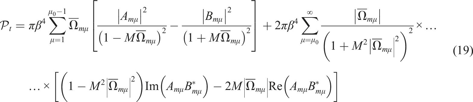
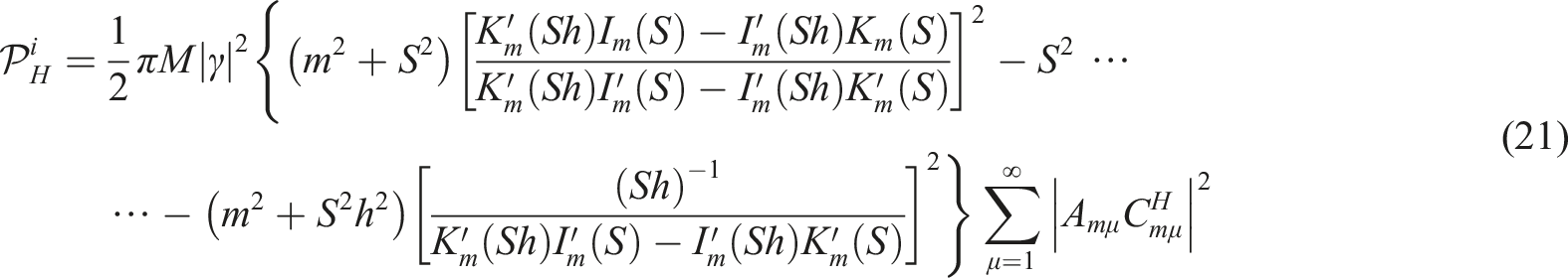
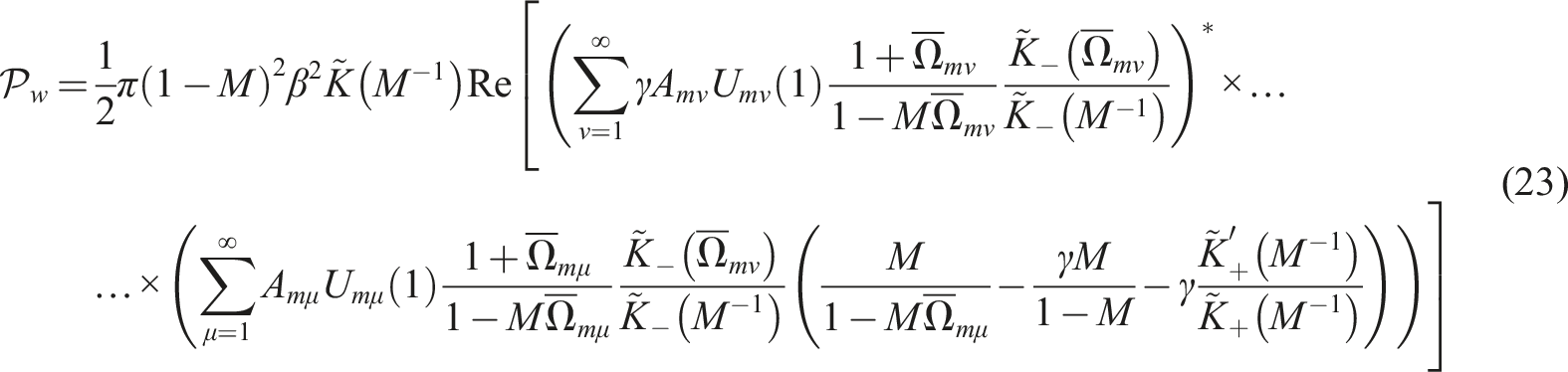
These are valid for any 0 $⩽$ h < 1. If h → 0, ${\mathcal{P}}_H^i$ simplifies to

$${\mathcal{P}}_H^i=\frac{1}{2}\pi M{\left|\gamma \right|}^2\left\{\left(m^2+S^2\right)\frac{I_m{\left(S\right)}^2}{I_m^{\prime }{\left(S\right)}^2}-S^2\right\}{\displaystyle \sum _{\mu =1}^{\infty }{\left|A_{m\mu }{C}_{m\mu }^H\right|}^2}$$

(21a)

Although the solution, equation (8), has no particularly simple form along the vortex sheet, still an explicit expression of ${\mathcal{P}}_w$ is possible, because the integral in x is just the Fourier transform of v (1, x) at Fourier variable S. A minor problem is that the integral is divergent and should be interpreted in a physically meaningful way. Furthermore, it is useful to note that $\tilde{K}\left(M^{-1}\right)$ is real, because

$$\tilde{K}\left(M^{-1}\right)=L\left(-\mathit{i}S\right)=\{\begin{array}{ll}-2K_m^{\prime }\left(S\right)\left(I_m^{\prime }\left(S\right)-\frac{I_m^{\prime }\left(Sh\right)K_m^{\prime }\left(S\right)}{K_m^{\prime }\left(Sh\right)}\right)\hfill & \text{if}\hspace{1em}h>0\hfill \\ -2K_m^{\prime }\left(S\right)I_m^{\prime }\left(S\right)\hfill & \text{if}\hspace{1em}h=0\hfill \end{array}$$

(24)

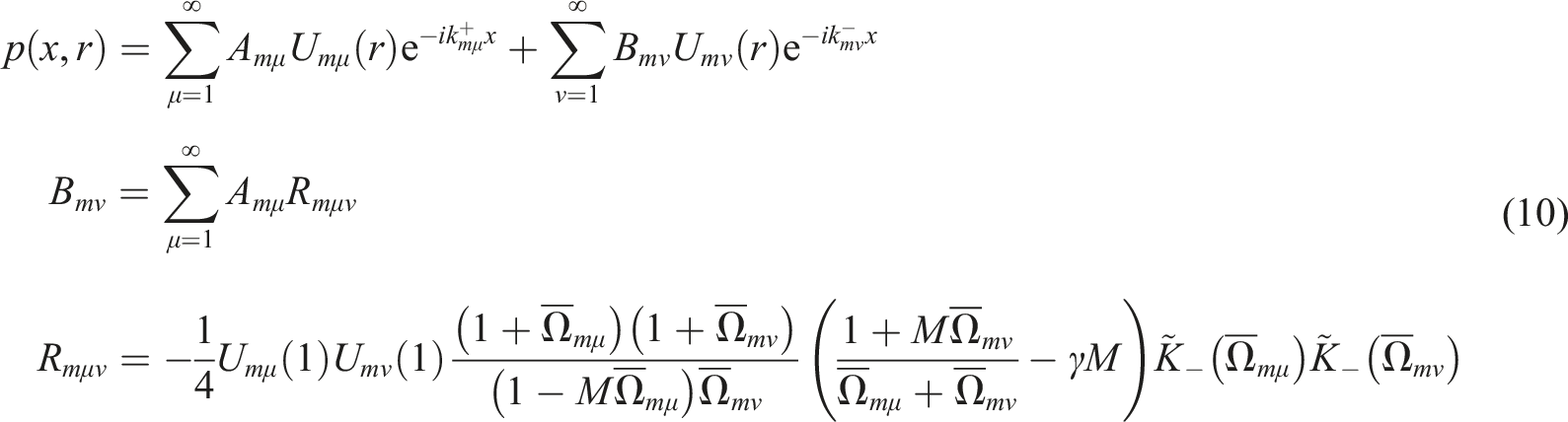
The above expressions are for a general incident field, made of a linear combination of radial modes of azimuthal order m. For the restricted case of a single incident μ-mode, we assume A _mμ = 1 and A _mν = 0 for all ν ≠ μ, and the expressions simplify accordingly.

Numerical details on the integration

The typical integral to determine the split functions ${\tilde{K}}_{\pm }\left(t\right)$ and their derivatives has the form

$${\displaystyle {\int }_0^{\infty }f}\left(\tau \right)\text{d}\tau$$

(25)

for a complex function f (τ) that is analytic in the upper halfplane, with a branch cut along [1, ∞), and a pole in τ = t possibly along the integration contour, or along the imaginary axis. To avoid the branch point and the poles we deform the contour from the positive real axis a little bit into the upper halfplane (Figure 2) according to

$$\tau =\sigma \left(\zeta \right)=\zeta +id\frac{q{t}_0^{q-1}\zeta }{\left(q-1\right)t_0^q+{\zeta }^q},\hspace{1em}0\mathrm{⩽}\zeta <\infty$$

(26)

Figure 2.

Examples of deformed integration contours in complex τ-plane.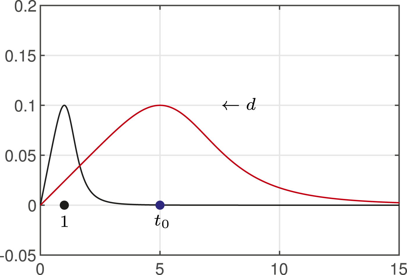

The deformed contour τ = σ starts at the origin τ = 0, then has an indentation of height d around τ = t₀ and returns to the real τ-axis for ζ → ∞ by a convergence rate of $\tau =\zeta +\mathit{i}O\left({\left(t_0/\zeta \right)}^{q-1}\right)$ . Finally, the contour is mapped to the unit interval by

$$\zeta \left(s\right)=\frac{s}{{\left(1-s\right)}^n},\hspace{1em}0\hspace{0.17em}\mathrm{⩽}\hspace{0.17em}s\hspace{0.17em}<1,$$

(27)

such that

$${\displaystyle {\int }_0^{\infty }f}\left(\tau \right)\text{d}\tau ={\displaystyle {\int }_0^{1}f}\left(\sigma \left(\zeta \left(s\right)\right)\right){\sigma }^{\prime }\left(\zeta \left(s\right)\right){\zeta }^{\prime }\left(s\right)\text{d}s$$

(28)

and f(τ) dτ ∼ τ⁻² log  τ dτ for τ → ∞ is turned into ∼ (1 − s)ⁿ⁻¹ log (1 − s) ds for s ↑ 1. The values used here are d = 0.1, q = 6 and n = 2, and the location of the indentation is taken $t_0=\max (1,\mathrm{R}\mathrm{e}\left(t\right))$ .

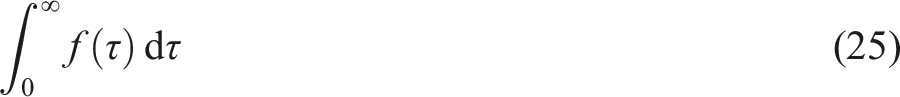
The other relevant integral is the power of the far field ${\mathcal{P}}_f$ , over the squared directivity |D _mμ (ξ)|². The integral is taken per lobe, from zero to zero, by a Gauss-Legendre integration scheme of 100 nodes which is (in general) enough for an accuracy of 10–14 digits. Only for m = 20 we had to increase to 200 nodes.

A survey of the power contributions

In order to assess the relative importance of the various power contributions, we made a survey of several configurations, all involving a full Kutta condition (γ = 1).

We made plots of the powers ${\mathcal{P}}_t,{\mathcal{P}}_f,{\mathcal{P}}_H^{\mathit{i}},{\mathcal{P}}_H^o,{\mathcal{P}}_w$ as a function of frequency, complemented for a few typical cases by the values given in their full numerical accuracy. As long as ${\mathcal{P}}_t-\left({\mathcal{P}}_f+{\mathcal{P}}_H^{\mathit{i}}+{\mathcal{P}}_H^{\mathit{o}}+{\mathcal{P}}_w\right)$ is very small we have a confirmation of the analytical and numerical correctness of the solution and its numerical implementation. The remaining difference should be in the order of the total numerical accuracy. Optimally, this is O(10⁻¹²), but of course it varies. A deterioration is seen, for example, for high m, high ω, frequencies very near cut-off, or Mach numbers close to unity.

For the interpretation of the graphs it is important to realize that there is a certain arbitrariness in the way the modes depend on frequency. The incident modes, and thus the resulting powers, are normalized on the pressure, more specifically on the mean squared modal function U _mμ (r). We could have normalized the incident potential or velocity, but we chose for pressure because this is what is normally measured. A normalization on the transmitted power ${\mathcal{P}}_t$ is obviously preferable, but this is simply not possible, because in some occasions ${\mathcal{P}}_t$ becomes zero or negative.

For most cases we used a single radial mode as incident field, because several modes at the same time is too general to be informative. However, for a numerical check a single mode case is less stringent because phase errors may remain unnoticed. Therefore we start with a sum of 5 radial modes, with A_m1 = ⋯ = A_m5 = 1, h = 0.5, m = 0 and m = 1, and M = 0 and M = 0.5 (Table 1 and Figure 3).

Table 1.

h = 0.5, sum over amplitudes A_m1 = ⋯ = A_m5 = 1. ${\displaystyle \sum \mathcal{P}}={\mathcal{P}}_f+{\mathcal{P}}_H^{\mathit{i}}+{\mathcal{P}}_H^o+{\mathcal{P}}_w$ . See Figure 3.

	M = 0, m = 0, ω = 3	M = 0.5, m = 0, ω = 3	M = 0.5, m = 0, ω = 8	M = 0.5, m = 1, ω = 3
${\mathcal{P}}_t$ ${\displaystyle \sum \mathcal{P}}$	+7.950756577684844+7.950756577683573	+8.881798462480251+8.881798462479171	+12.04433506608146+12.04433487934420	+6.261453561753953+6.261453561964006
${\mathcal{P}}_f$ ${\mathcal{P}}_H^i$	+7.950756577683573+0.000000000000000	+6.911117043933849+2.127020691414524	+7.912821216168379+1.698062708322932	+3.604346605067720+1.785364700094981
${\mathcal{P}}_H^o$ ${\mathcal{P}}_w$	+0.000000000000000+0.000000000000000	+1.475884116866221–1.632223389735423	+1.498003567612718+0.935447387240170	+1.274305293191131–0.402563036389825

Figure 3.

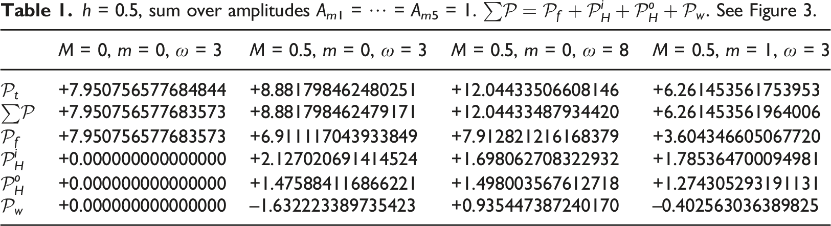
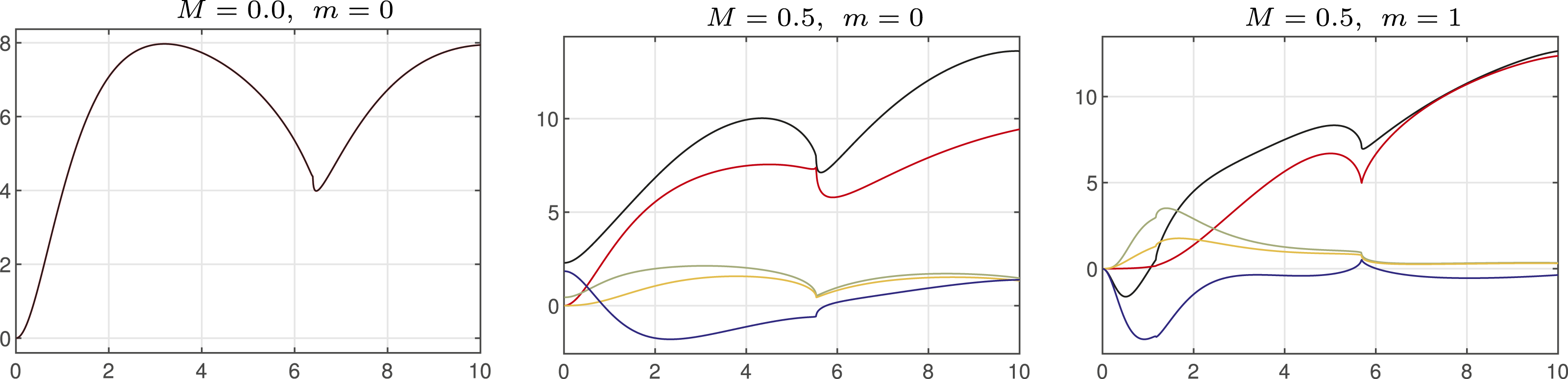
h = 0.5, sum over amplitudes A_m1 = ⋯ = A_m5 = 1, for frequency ω ∈ (0, 10]. Powers ${\mathcal{P}}_t$ = black, ${\mathcal{P}}_f$ = red, ${\mathcal{P}}_H^i$ = green, ${\mathcal{P}}_H^o$ = yellow, ${\mathcal{P}}_w$ = blue. See Table 1.

We see from the table, evaluated at ω = 3, that without mean flow, ${\mathcal{P}}_t$ and ${\mathcal{P}}_f$ are (within the numerical accuracy) the same. With mean flow, ${\mathcal{P}}_t$ is equal to the remaining powers, indicated in the table by ${\displaystyle \sum \mathcal{P}}={\mathcal{P}}_f+{\mathcal{P}}_H^{\mathit{i}}+{\mathcal{P}}_H^o+{\mathcal{P}}_w$ . This is exactly as it should. All in all this gives us a very high confidence of the formulas. (Note that in particular ${\mathcal{P}}_w$ is mathematically not incontrovertible, as it is the result of a non-convergent integral which has to be interpreted in a physically meaningful way.)

Figure 3 shows the behavior as a function of ω. Most interesting is the fact that for many frequencies ${\mathcal{P}}_w$ is negative, indicating energy production by the wake. Remarkably, this production is, for low enough frequency and m = 1, strong enough to render ${\mathcal{P}}_t$ negative.

In Table 2 and Figure 4 we present a series of configurations with m = 0, incident radial modes μ = 1, = 2, = 3, h = 0.0, and M = 0.0, = 0.2, = 0.5, = 0.8. For all incident modes except the plane wave (mμ = 01), ${\mathcal{P}}_w$ is negative for low enough ω. As could be verified from the formulas, if m = 0, ${\mathcal{P}}_H^i$ tends to a finite value for ω → 0, in contrast to ${\mathcal{P}}_H^o$ which tends to zero. This is interesting for the plane wave case (1st column of Figure 4). For M = 0 the exit is “closed” and ${\mathcal{P}}_t={\mathcal{P}}_f\to 0$ . For any M > 0 the shedding of vorticity reduces the reflection coefficient and effectively “opens” the exit. As a result ${\mathcal{P}}_t\to 4\pi M$ remains now finite for ω → 0. This is balanced by ${\mathcal{P}}_H^i$ only, since ${\mathcal{P}}_f$ , ${\mathcal{P}}_w$ and ${\mathcal{P}}_H^o$ still vanish.

Table 2.

m = 0, h = 0.0, M = 0.2 at ω = 1. See Figure 4.

μ	1	2	3	4
${\mathcal{P}}_t$	+3.576185456995646	+0.534981991515257	+0.215233977630079	+0.059890681780837
${\displaystyle \sum \mathcal{P}}$	+3.576185456995588	+0.534981991515217	+0.215233977630038	+0.059890681780802
${\mathcal{P}}_f$	+1.723284029432968	+0.118755082602218	+0.065292372266931	+0.045514909392450
${\mathcal{P}}_H^i$	+0.563373304414484	+0.285622492444845	+0.291053617393213	+0.248217438274667
${\mathcal{P}}_H^o$	+0.372358765156304	+0.188780756479334	+0.192370431324303	+0.164058073185194
${\mathcal{P}}_w$	+0.917169357991832	−0.058176340011180	−0.333482443354409	−0.397899739071509

Figure 4.

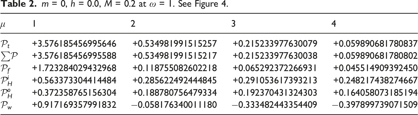
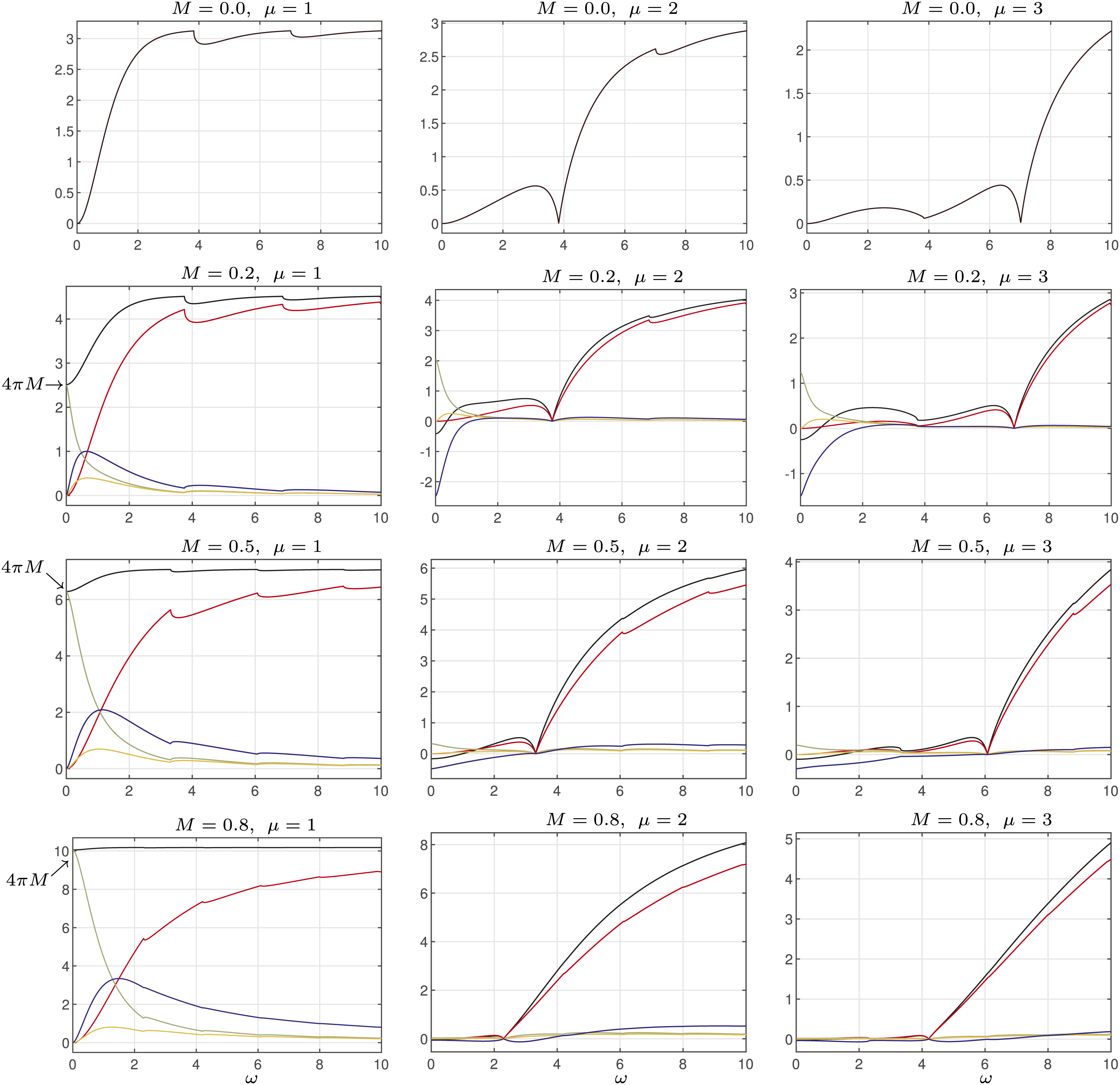
m = 0, h = 0.0, M = 0.0, 0.2, 0.5, 0.8, and incident modes μ = 1, 2, 3. Powers ${\mathcal{P}}_t$ = black, ${\mathcal{P}}_f$ = red, ${\mathcal{P}}_H^i$ = green, ${\mathcal{P}}_H^o$ = yellow, ${\mathcal{P}}_w$ = blue, for frequency ω ∈ (0, 10]. See Table 2.

For other than the plane wave modes (the 2nd and 3rd columns of Figure 4), ${\mathcal{P}}_w$ may be negative but (and this is more surprising) also ${\mathcal{P}}_t$ if ω is small enough. Apparently, the shed vortices produce (low frequency and therefore long) sound waves that do not radiate away since the scattering duct exit is a compact and therefore inefficient source. Instead, they propagate upstream into the duct on the backward running cut-on plane wave mode, yielding a negative ${\mathcal{P}}_t$ .

Another phenomenon of interest is the important role played by the cut-off frequency of the incident mode (i.e. where ${\overline{\mathrm{\Omega }}}_{m\mu }$ = 0). Except for the plane wave (with cut-off frequency ω = 0), all power contributions vanish there. Mathematically, this is mainly due to the vanishing of ${\tilde{K}}_{-}\left({\overline{\mathrm{\Omega }}}_{m\mu }\right)$ .

For high frequencies the sound waves become ray-like and the part of the field that interacts with the edge becomes smaller and smaller. It is therefore no surprise that for ω → ∞ the power contributions are dominated by ${\mathcal{P}}_t\simeq {\mathcal{P}}_f$ .

In Table 3 and Figure 5 we present a series of configurations with m = 1, incident radial modes μ = 1, = 2, = 3, h = 0.5, and M = 0.0, = 0.2, = 0.5, = 0.8. Again for all incident modes except the first (mμ = 11), ${\mathcal{P}}_w$ is negative for low enough ω. An interesting feature is that for M = 0.5, μ = 3, there is an interval in ω, where ${\mathcal{P}}_t<0$ and ${\mathcal{P}}_f>0$ and are both non-negligible. Apparently, the production of sound by the mean flow through the wake ( ${\mathcal{P}}_w$ is big negative) is strong enough for radiation of sound upstream into the duct and to the far field.

Table 3.

m = 1, h = 0.5, M = 0.5, ω = 1.5. See Figure 5.

μ	1	2	3	4
${\mathcal{P}}_t$	+1.941885698925230	−0.003965563040558	−0.047460548206990	−0.041399789727046
${\displaystyle \sum \mathcal{P}}$	+1.941885698928027	−0.003965563044226	−0.047460548208855	−0.041399789728307
${\mathcal{P}}_f$	+0.610604821641485	+0.037775452326324	+0.021183079414968	+0.014612502774287
${\mathcal{P}}_H^i$	+0.540301406674775	+0.173641314199742	+0.115511672314417	+0.082633275388866
${\mathcal{P}}_H^o$	+0.269075913121263	+0.086475242515879	+0.057526055494567	+0.041152260117738
${\mathcal{P}}_w$	+0.521903557490504	−0.301857572086170	−0.241681355432807	−0.179797828009197

Figure 5.

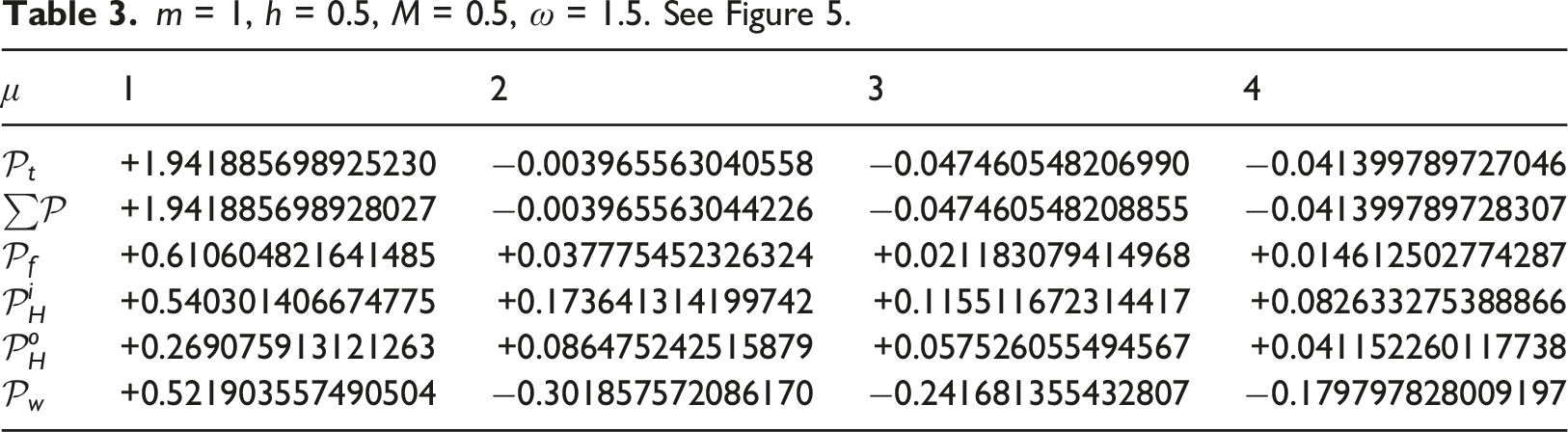
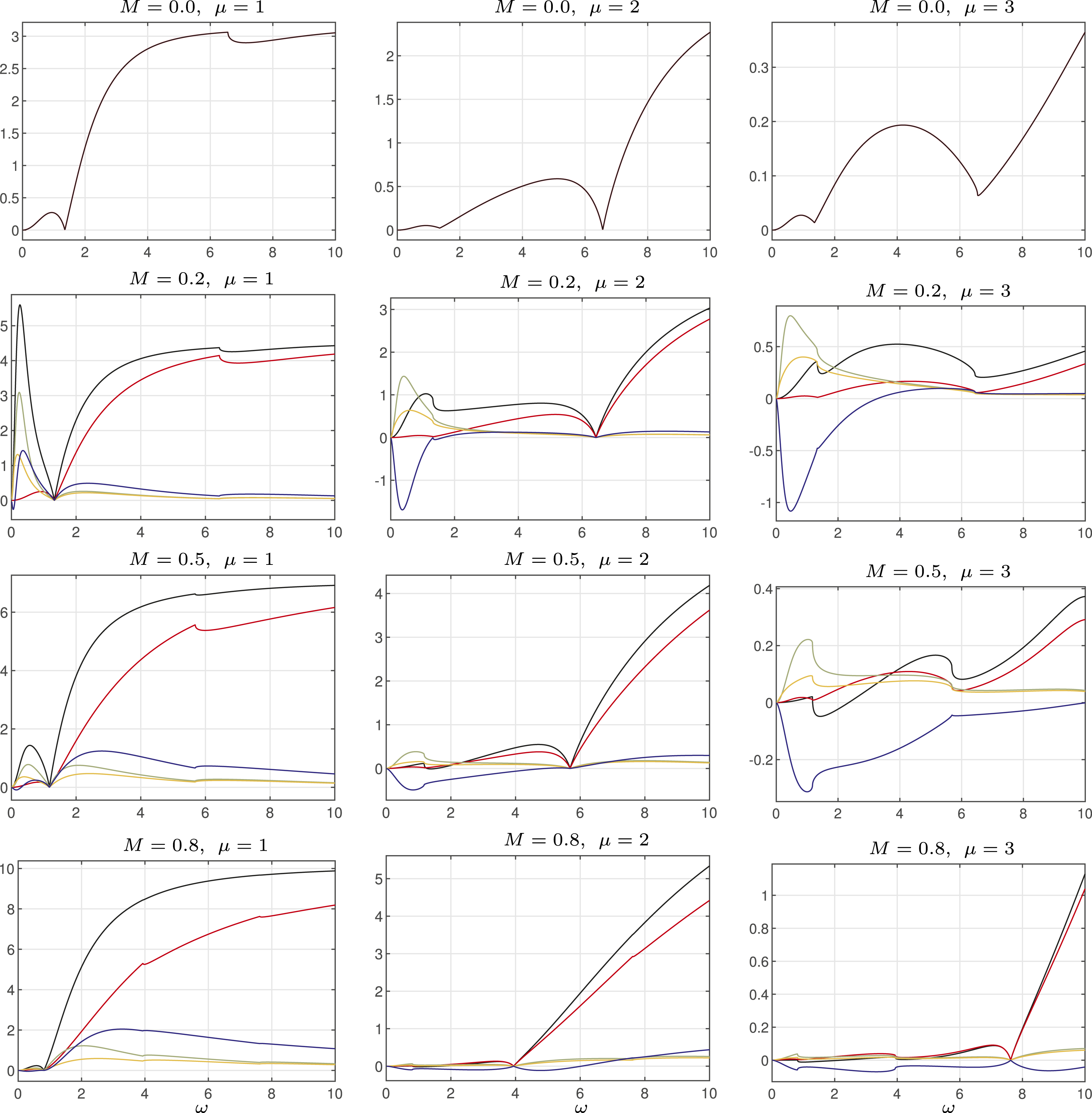
m = 1, h = 0.5, M = 0, 0.2, 0.5, 0.8, and incident modes μ = 1, 2, 3. Powers ${\mathcal{P}}_t$ = black, ${\mathcal{P}}_f$ = red, ${\mathcal{P}}_H^{\mathrm{i}}$ = green, ${\mathcal{P}}_H^o$ = yellow, ${\mathcal{P}}_w$ = blue, for frequency ω ∈ (0, 10]. See Table 3.

The first mode is cut-off under (roughly) ω ≃ 1, and in general (M = 0 or M⩾0.5) not much energy is passing the exit. However, for small Mach numbers (like M = 0.2), a large amount of acoustic energy in the duct is used for the vortex shedding, but without radiating to the far field. This is different from the previous case of m = 0 (Figure 4), because now the production from the duct field ${\mathcal{P}}_t$ is turned into both the hydrodynamic field inside ${\mathcal{P}}_H^{\mathit{i}}$ and outside ${\mathcal{P}}_H^o$ the jet, and absorbed by the ${\mathcal{P}}_w$ , instead of only the inside part ${\mathcal{P}}_H^{\mathit{i}}$ . Moreover, it happens only for small Mach numbers.

Finally, we consider also high m-number cases in Table 4 and Figure 6. The values chosen are m = 20, h = 0.0, with M = 0.0 for μ = 1…3, and M = 0.2 for μ = 1…6. In all case the strong r²⁰ behavior of the field in the duct blocks the radiated field almost completely for (say) ω < 15. The transmitted power ${\mathcal{P}}_t$ is then also vanishing for M = 0.0, but not at all for M = 0.2. Similar to the case for m = 1 discussed above, the production from the duct field ${\mathcal{P}}_t$ is turned into the hydrodynamic fields inside ${\mathcal{P}}_H^i$ and outside ${\mathcal{P}}_H^o$ and absorbed by the wake ${\mathcal{P}}_w$ . Due to the high m-value, the incident field is concentrated to the duct wall region. This makes the role of the edge symmetric for inside and outside, with the result that ${\mathcal{P}}_H^i$ and ${\mathcal{P}}_H^o$ are practically equal and almost non-distinguishable in the graphs.

Table 4.

m = 20, h = 0.0, M = 0.2, ω = 5 (top), =25 (bottom), incident modes μ = 1, 2, 3, 6. See Figure 6.

μ	1	2	3	6
${\mathcal{P}}_t$	+1.625566427644335	+0.472163008825096	+0.290415752254500	+0.120477585028266
${\displaystyle \sum \mathcal{P}}$	+1.625566427644079	+0.472163008825004	+0.290415752254433	+0.120477585028224
${\mathcal{P}}_f$	+8.6901617649e−21	+2.4680297608e−21	+1.5813419842e−21	+8.1208181997e−22
${\mathcal{P}}_H^i$	+0.446397934256077	+0.161450255619367	+0.117437082035453	+0.073616621554546
${\mathcal{P}}_H^o$	+0.440330647332084	+0.159255879369784	+0.115840917677271	+0.072616049797665
${\mathcal{P}}_w$	+0.738837846055918	+0.151456873835853	+0.057137752541709	−0.025755086323987

μ	1	2	3	6
${\mathcal{P}}_t$	+1.661575103643486	+0.189417602093594	+0.088705444382308	+0.054465324851519
${\displaystyle \sum \mathcal{P}}$	+1.661575103642349	+0.189417602093297	+0.088705444382049	+0.054465324851371
${\mathcal{P}}_f$	+1.490131664087533	+0.153596746287418	+0.056668025740713	+0.022060513522550
${\mathcal{P}}_H^i$	+0.042193832300105	+0.009925108755137	+0.009025089168765	+0.009627522115405
${\mathcal{P}}_H^o$	+0.041565199911696	+0.009777237739829	+0.008890627256905	+0.009484084748094
${\mathcal{P}}_w$	+0.087684407343015	+0.016118509310913	+0.014121702215666	+0.013293204465322

Figure 6.

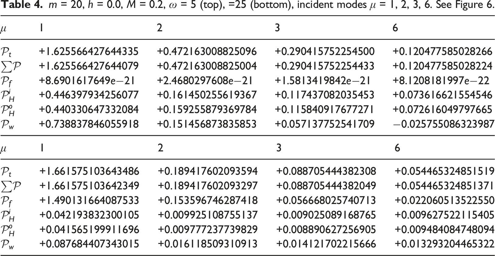
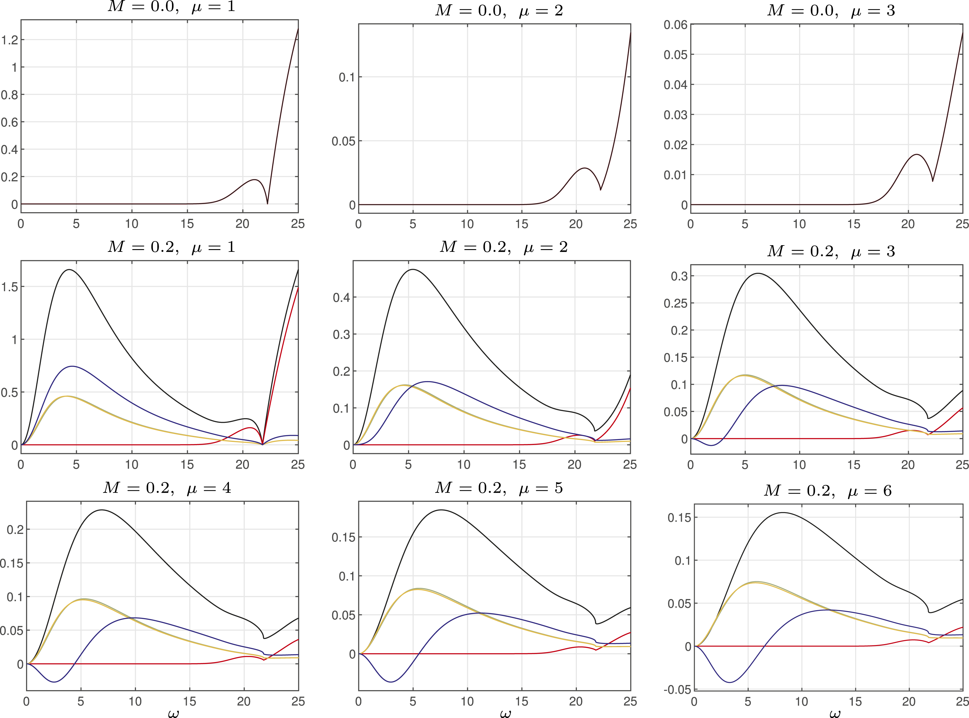
m = 20, h = 0.0, M = 0.2, incident modes μ = 1…6. For comparison 3 modes at M = 0.0. Powers ${\mathcal{P}}_t$ = black, ${\mathcal{P}}_f$ = red, ${\mathcal{P}}_H^{\mathit{i}}$ = green, ${\mathcal{P}}_H^o$ = yellow, ${\mathcal{P}}_w$ = blue, for frequency ω ∈ (0, 25]. ${\mathcal{P}}_H^i$ and ${\mathcal{P}}_H^o$ are practically equal and almost non-distinguishable. See Table 4.

Conclusions

Acoustic energy in mean flow is in general not conserved, as was shown conclusively by Myers. ¹⁹ Energy may be produced by or disappear into vorticity or entropy. In particular in the case of production there must be an exchange with the energy of the mean flow, because there is no other source. One way to study this is by model problems that are simple enough for analytically exact energy expressions and can be evaluated without approximation. The simplest (to our knowledge) of such model problems is the convective Sommerfeld problem of plane waves diffracting at a half plane with uniform mean flow. ¹⁴ The absorption of energy by the wake of shed vortices has a remarkable simple form and it is easy to show that it can be both positive and negative, depending on Mach number and angle of incidence. However, the vortices are shed by incident plane waves with, in principle, an infinite content of acoustic energy. So it is still hard to compare the amount of dissipated energy with the incident energy, and in particular to conclude if and how much of the energy must be produced by the mean flow.

Therefore it is interesting to revisit the next simplest model problem, namely of sound radiated from a semi-infinite duct with uniform mean flow. ¹⁶ Here the incident energy carried by the duct modes is definitely finite, but otherwise the various contributions are very similar as in the convective Sommerfeld problem.

Although the energy components (power transmitted through the duct ${\mathcal{P}}_t$ , far field ${\mathcal{P}}_f$ , hydrodynamic fields inside ${\mathcal{P}}_H^{\mathit{i}}$ and outside ${\mathcal{P}}_H^o$ the vortex sheet, and the power absorbed by the wake ${\mathcal{P}}_w$ ) were presented (as part of the Wiener-Hopf solution for the acoustic field) long ago, it was, due to not altogether straightforward numerical evaluation, never studied in any detail other than for a single sample case (a “proof of concept”).

In the present paper we filled this lacuna and gave a survey of the various energy components as function of frequency and other problem parameters. The main conclusions are that (i) the global energy conservation ${\mathcal{P}}_t={\mathcal{P}}_f+{\mathcal{P}}_H^{\mathit{i}}+{\mathcal{P}}_H^o+{\mathcal{P}}_w$ is recovered in all cases leading to the conclusion that the formulas are correct; (ii) for high frequencies the energy bookkeeping is dominated by the transmitted power ${\mathcal{P}}_t$ and the radiated power ${\mathcal{P}}_f$ ; (iii) for lower frequencies there is a strong interaction between all contributions often leading to negative ${\mathcal{P}}_w$ (energy produced by the wake) and sometimes a negative ${\mathcal{P}}_t$ (so much energy is produced that more propagates back into the duct than was used for its creation).