Sage Journals: Discover world-class research

Abstract

This paper presents an optimisation approach for designing low-noise Outlet Guide Vanes (OGVs) for fan broadband noise generated due to the interaction of turbulence and a cascade of 2-dimensional aerofoils. The paper demonstrates the usage of Bayesian optimisation with constraints to reduce the computation cost of optimisation. The prediction is based on Fourier synthesis of the impinging turbulence and the aerofoil response is predicted for each vortical modal component. A linearised unsteady Navier-Stokes solver is used to predict the aerofoil response due to an incoming harmonic vortical gust. This paper shows that to achieve noise reductions of 0.5 dB the penalty on the aerodynamic performance of 33% is observed compared to baseline aerofoil. Hence, the geometry changes such as thickness and nose radius can’t reduce broadband noise without effecting aerodynamic performance.

Keywords

Bayesian optimisation fan broadband noise turbulence-aerofoil interaction noise low-noise aerofoil

Introduction

The broadband noise due to the interaction between the rotor wake and the downstream Outlet Guide Vanes (OGV) is the major component of fan noise from an aircraft engine, especially at approach conditions. Recent flightpath 2050 targets have been set aimed at reducing noise emissions by 65% by 2050. One of the possible ways to reduce the interaction noise is by modifying the 2 D aerofoil geometry. Given Outlet guide vanes (OGV) serve the purpose of reducing swirl from the flow that exit the fan, its aerodynamic performance is a key parameter.

In a typical turbofan engine the OGV has aerofoils that are closely spaced at a separating distance (spacing) almost equal to their chords. Acoustic interactions between the blades therefore become a significant factor in the acoustic response to incident turbulence. The single aerofoil approach cannot account for interactions between the vanes of an OGV across the full range of frequencies of interest.

In 1958 a two-dimensional unwrapped blade row was considered by Lane and Friedman¹ in an analysis of the unsteady lift and moment on compressor and turbine blades for the prediction of flutter rather than noise. Torsional flutter was also the subject of work by Whitehead² where a chord-wise distribution of bounded vorticity is described on the blade surfaces. The reaction of the bounded vorticity and their shed vortices are combined to form a description of the unsteady blade forces.³ Kaji and Okazaki developed a model for the tonal noise generated due to the potential and velocity deficit interactions between a stator row and downstream rotor. Their formulation replaced the blade row with a distribution of pressure doublets, the strength of which were determined by the numerical solution of an integral equation.

In 1973, Smith⁴ used a bounded vorticity approach, similar to that seen in Whitehead, in order to obtain an integral equation for the unknown vorticity distribution along the cascade blades. Expressions were given for the calculation of the distribution of unsteady forces and moments and acoustic pressure due to blade torsion and translation and incident acoustic and vorticity waves. Solutions to the integral equation were obtained using a collocation technique. Further details of this theory and a FORTAN code to compute the cascade response based on this formulation, LINSUB, were presented in 1987 by Whitehead.⁵

The analyses of Kaji and Okazaki,³ Smith,⁴ Whitehead ⁵ mentioned above all employ numerical schemes in order to obtain their solutions, introducing significant computational difficulties at high frequencies. Approximate analytic expressions for the sound transmission through a two-dimensional cascade were presented in 1970 by Mani and Horvay⁶ Their approach was based on the Wiener-Hopf technique and neglected interaction between the leading and trailing edges by using semi-infinite blades for both the downstream-propagating waves from the leading edges and upstream-propagating waves from the trailing edge. These wave interactions were resolved in the vane overlap region, thus limiting this technique to overlapping configurations.

Since 1992 further developments have been undertaken by Peake and co-workers. The unsteady blade loading due to an incident vortical gust was calculated by Peake^7,8 The upstream radiation of sound waves at non-zero angle of attack was obtained using similar techniques by Peake and Peake and Kerschen⁹ whilst the effects of small amounts of blade thickness and camber are considered theoretically by Evers and Peake¹⁰ They showed that the blade geometry effects on the radiated power is significant by interaction with a single gust, whereas in case of turbulence-cascade interaction the aerofoil geometry effects are within 2 dB in comparison with flat plate.

The numerical approach to the cascade problem was extended to predictions of broadband noise in 1998 by Hanson and Horan¹¹ using the 3 D harmonic cascade response function developed by Glegg^12,13 In 2006, Cheong et al.¹⁴ exploited the periodicity in the harmonic cascade response function, used to obtain a relatively efficient formulation of the broadband noise from 2 D cascades by re-ordering the summations over vortical mode index and scattering index.

More recently Polacsek et al.¹⁵ presented a three-dimensional computational hybrid method aiming at simulating the acoustic modes from an ducted annular cascade subjected to a prescribed homogeneous isotropic turbulent flow. The predicted fluctuating pressures over the aerofoil were used as the input to a Ffowcs Williams and Hawkings integral solver to calculate the radiated sound field. This analysis is limited to plane mode in the azimuthal direction.

Previously, Chaitanya et al.¹⁶ demonstrated the prediction of turbulence-cascade interaction noise in 2 D using a Fourier mode decomposition of the incoming turbulence in the azimuthal direction. No span-wise correlation effects were therefore included in the 2 D approach. This approach entails calculating sound power over a number of ’strips’ across the span of the OGV (whose strip size is greater than turbulence integral length scale) and then summing them all up to compute the overall sound power. These observations are consistent with experimental work of Chaitanya et al., ^17,20 who demonstrated ft/U (t is the maximum aerofoil thickness) is the important noise reduction parameter with reference to flat plate.

Recently, Gea-Aguilera et al.¹⁹ investigates the influence of various fan wake modelling assumptions on turbulence-cascade interaction noise. Two-dimensional CAA simulations are performed using the LEEs and synthetic turbulence with isotropic turbulence and cyclostationary variations in the TKE and TLS. A systematic parameter study on noise has been performed, including variations in the vane count, aerofoil thickness, camber, mean flow Mach number, stagger angle, and inter-vane spacing. It has been shown up to 2 dB variation in sound power level is observed with the parameters chosen in the study.

One of the key objective of this paper is to design a low-noise OGV within acceptable aerodynamic constraints using a machine learning based approaches. Recently, Chaitanya et al.¹⁶ demonstrated the frequency domain calculation for the radiated sound power is very expensive. In order, to reduce the computational cost, here in this work we intend to apply the Bayesian optimisation framework to optimise the OGV design for low broadband noise.

Bayesian optimisation^21,22 is a powerful probabilistic framework for efficient global optimisation of expensive black-box functions. The field has been applied to a wide range of applications recently including material science³⁵ neuroscience,^24–26 and robotics²⁷ and has contributed to improved efficiency in optimisation especially for expensive processes. The field has offered a diverse set of algorithms that meet specific design needs²² Bayesian optimisation has been shown converge and gives a reduction in the computational cost. In this paper, for the first time, we use Bayesian optimisation to design low-noise OGV with aerodynamic considerations.

In this paper, we also developed theoretical framework by which turbulence-cascade broadband interaction noise can be predicted in 2 dimensions using a linearized Navier-stokes solver and a Fourier turbulence description. The preliminary results are presented in the conference version of the paper.²³

Problem definition

Low-noise OGV design optimisation is performed on a baseline OGV geometry of Modular Fan Rig (MFR) of AneCom Aerotest, Wildau, Germany. The scaled 34” diameter fan referred to as ACAT R1 rotor. The fan stage consists of a rotor with 20 blades and a stator with 44 OGVs. The simulations in the present study are performed at two operating conditions similar to the acoustic certification points approach (AP) and sideline (SL) conditions. The current low-noise optimisation is performed at approach condition. To ensure the newly designed OGV doesn’t have any significant aerodynamic penalty, aerodynamic performance is evaluated at sideline condition and used as a design constraint in optimisation routine. Due to computation cost, the current optimisation is performed at different radial 2 D cuts af 10, 25, 50, 75 and 90% of span are considered in this study.

Flow chart

Figure 1 shows a schematic block diagram of the optimisation process. The procedure to estimate the radiated sound power is divided into two steps. First step involves the non-linear HYDRA simulation (RANS solver) which calculates the mean flow around the aerofoil. The second step involves using the predicted mean flow in step 1 as input to the Linearized Navier-Stoke (LNS) solver to predict the noise. Turbulence parameters such as turbulent intensity and length scales are extracted from RANS simulations which are used to synthesised the turbulence and provide input to LNS solver. Aerodynamic performance parameters such as pressure loss and flow exit angle are calculated from RANS simulations for sideline (cruise) condition. More details about the HYDRA solver and turbulence synthesis is illustrated in later sections of the paper.

Figure 1.

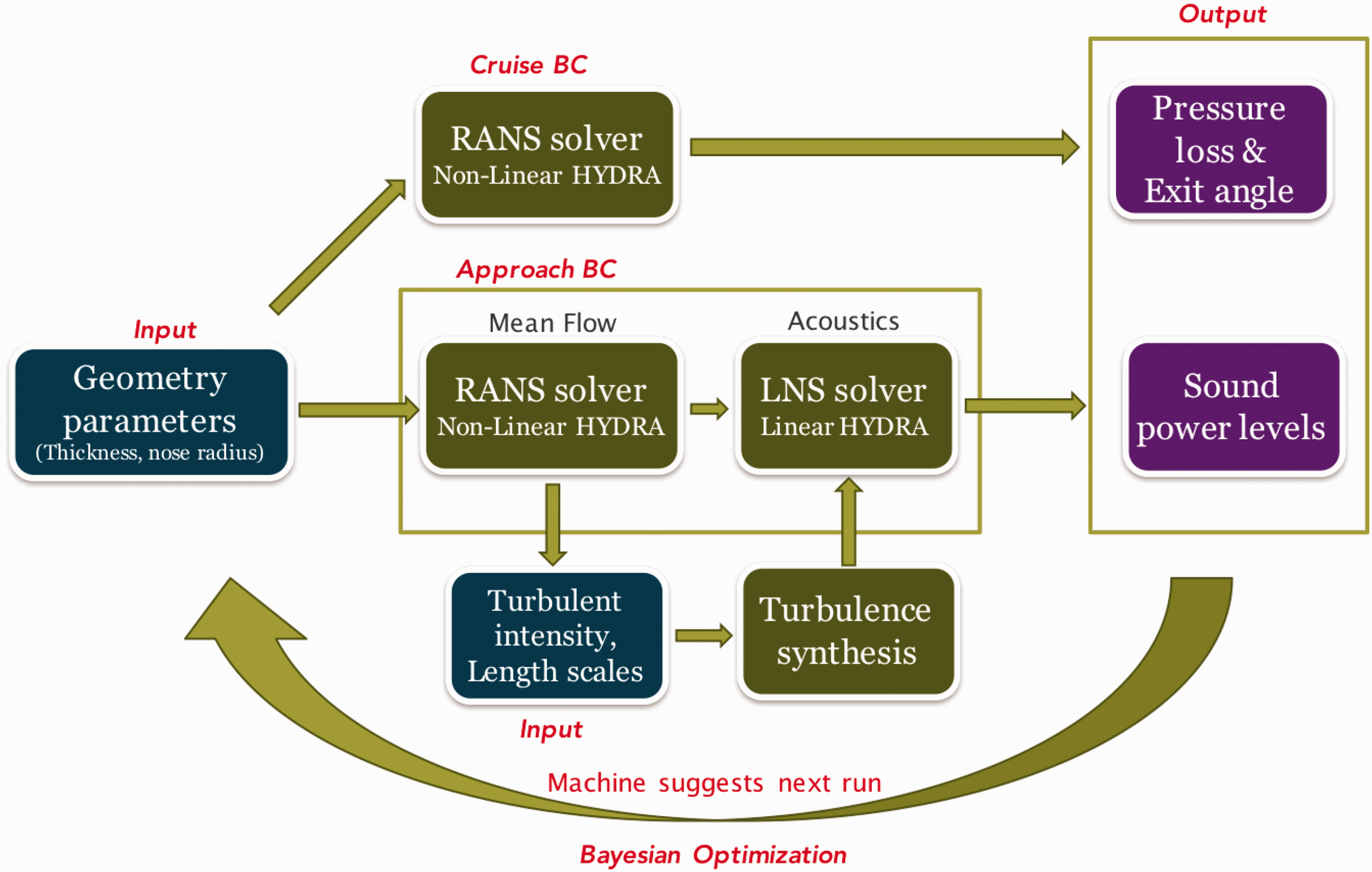
Flow chart of the optimisation process.

The noise calculations using LNS frequency domain solver are very expensive as the simulations need to be performed at each frequency and each azimuthal mode number (will be further explained). Hence, in this paper, machine learning based approach ’Bayesian optimisation’ is used to reduce the computational cost. The output parameters (sound power level, pressure loss and exit angle) for each aerofoil geometry configuration are used in the Bayesian optimisation routine and machine recommends the next aerofoil configuration to consider.

Input and output parameters

OGV 2 D profile is parameterised by 9 geometric parameter, i.e. 1) Leading Edge nose radius r, 2) Ellipse a/b Ratio, 3) Leading Edge Ellipse” eccentricity” e, 4) Trailing Edge Circle Diameter, 5) Maximum Thickness t, 6) Location of Maximum Thickness, 7) Leading Edge Camber Angle θ_LE, 8) Trailing Edge Camber Angle θ_TE and 9) Chord length c₀. In this paper we only vary two parameters such as thickness and nose radius as these have an moderate effect on broadband noise.^17,20 The ellipse shape and eccentricity is kept constant but the ellipse ratio is changed due to change in nose radius. In order to keep the same ellipse shape, chord is slightly varied. Maximum thickness location, trailing edge circle diameter has very negligible influence of broadband noise and hence the current approach is restricted to two parameters.¹⁸ One of the primary objective of the paper is shown the advantages of Bayesian optimisation over conventional optimisation.

In the present study, a total of 36 different configurations are considered with different combinations of normalised thickness and normalised nose radius varying from (0.5, 2.5) and (0.5, 2) in steps of 0.25 and 0.5 respectively. Please note that these are normalised over baseline thickness and nose radius parameters.

The key output parameters are radiated sound power levels, pressure loss across the OGV and flow exit angle. Please note, the sound power levels are predicted at approach condition and pressure loss and flow exit angles at sideline condition.

Numerical approach

The 3 D viscous CFD solver used in the present study is the Rolls-Royce plc code, HYDRA. HYDRA is a suite of non-linear and linear unsteady solvers which uses efficient second-order edge-based discretisation on unstructured hybrid grid.^28,29 A 5 step Runge-Kutta algorithm, with an element collapsing multi-grid accelerator algorithm is used iteratively to converge to a steady state solution. Domain decomposition is used to run the solver in parallel on both shared and distributed memory machines.

Steady flow simulations

The accurate prediction of the mean flow around the aerofoil is highly crucial to capture the gust distortion due to mean flow gradients around the stagnation region of the aerofoil. In the present study the steady Reynolds Averaged Navier-stokes (RANS) solver as a part of HYDRA is used to obtain the mean flow around the aerofoil geometry. The $k - ω$ turbulence model is used. The limitation of the present scheme is its limited accuracy for separated flows.

Linear unsteady CFD simulations

The linear unsteady CFD HYDRA module (HYDLIN) is based on a full linearisation of the Navier-Stokes equation. The unsteady problem is solved in the frequency domain for the complex flow amplitudes, $\hat{q} (x)$ . A pseudo-time derivative is introduced into the linear equation to enable the same numerical methods adopted for the non-linear CFD code to be used to converge the linear unsteady solution.

q (x, t) = \bar{q} (x) + \hat{q} (x) e^{i ω t}

(1)

Mesh generation and boundary conditions for unsteady simulations

The mesh generation is performed using the Rolls-Royce in-house software PADRAM. An H–O–H mesh topology is used to grid a single OGV passage with the cascade effect simulated by imposing a periodic boundary condition at the upper and lower walls. Subsonic inlet and outlet boundary conditions are imposed at inlet and outlet boundary and the viscous wall boundary condition on the aerofoil surface. The mesh uses a structured multi-block arrangement with a O-mesh of quadrilaterals cells around the OGV surface and H-meshes above and below the O-mesh and in the inlet and outlet flow region. The mesh density is taken to be sufficiently fine such that the HYDLIN code captures all the propagating cut-on acoustic modes. A number of different grid sizes are considered depending on the frequency of interest.

Non-reflecting boundary conditions based on an Eigenmode analysis of the unsteady flow field are applied at the inflow/outflow boundaries in order to minimise spurious reflections from the boundary.^30,31

Turbulence synthesis

Fourier description of the radiated sound power from 2 D aerofoil cascades

We start with developing the basic equations for predicting the spectrum of acoustic power due to a two-dimensional cascade of aerofoils following the Fourier approach of Cheong et al.¹⁴ A two-dimensional cascade of aerofoils with leading and trailing edge angles θ_LE and θ_TE are situated in a two-dimensional uniform mean flow with an incoming flow angle θ as shown in Figure 2.

Figure 2.

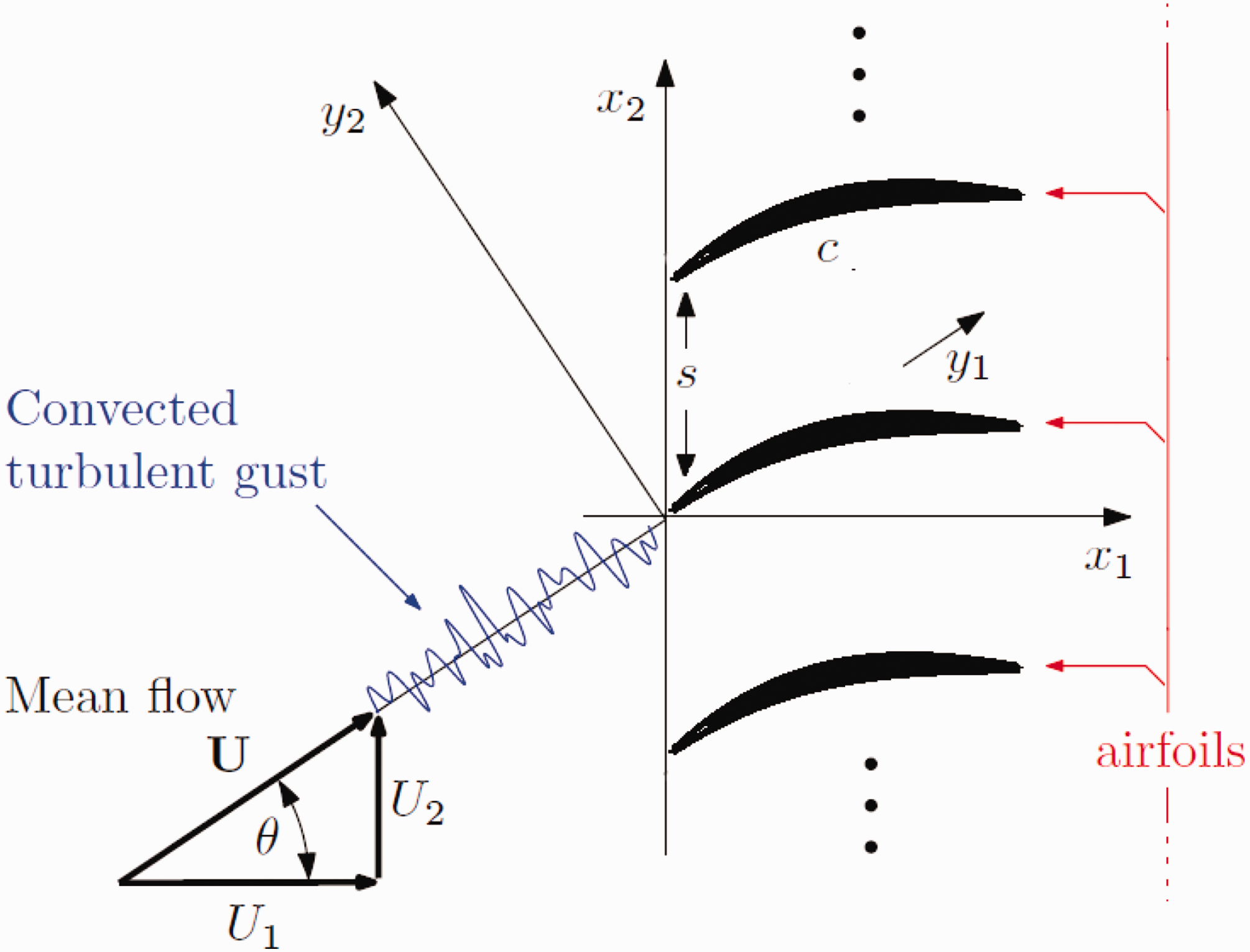
The convected turbulence gust interacting with cascade of aerofoils.

Consider a single incoming harmonic vortical gust impinging onto the cascade of aerofoils with velocity component u normal to the flow direction is of the form,

u (y_{1}, y_{2}, t) = u_{2} e^{i (k_{1} y_{1} - ω t + k_{2} y_{2})}

(2)

The acoustic pressure propagating upstream and downstream of the aerofoil cascade due to the single vortical mode can be expressed as the sum of a number of scattered acoustic modes. In this paper we define a non-dimensional pressure amplitude $R_{r}^{\pm}$ that is consistent with the amplitude definition for a flat plate cascade. The upstream and downstream acoustic pressure can therefore be written in the same form as for a flat plate cascade,

p^{\pm} (x_{1}, x_{2}, t) = ρ_{0} U u_{2} \sum_{r = - \infty}^{\infty} R_{r}^{\pm} e^{i (- k_{1} U t + α_{r} x_{1} + β_{r} x_{2})}

(3)

where u₂ is the unsteady velocity amplitude at the blade leading edge normal to the flow direction and α_r and β_r are the axial and circumferential acoustic wave numbers of the r^th acoustic wave The non-dimensional amplitudes

R_{r}^{\pm}

are readily calculated for a flat plate cascade using, for example, the co-location method developed by Smith and Whitehead or the Wiener-Hopf solution developed by Glegg^12,13 However, for a cascade of realistic aerofoils, the blade response is a complex function of blade geometry and angle of attack and must generally be computed using CFD methods.

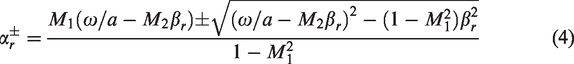
Substituting the form of the acoustic pressure of equation (3) into the Euler equation yields an expression for the axial acoustic wavenumber α_r given by

α_{r}^{\pm} = \frac{M_{1} (ω / a - M_{2} β_{r}) \pm \sqrt{{(ω / a - M_{2} β_{r})}^{2} - (1 - M_{1}^{2}) β_{r}^{2}}}{1 - M_{1}^{2}}

(4)

which defines a cut-on condition for the lth acoustic mode give by,

{(ω / a - M_{2} β_{l})}^{2} \geq (1 - M_{1}^{2}) β_{l}^{2}

(5)

where to ensure periodicity of the acoustic solution over the cascade we must have

β_{l} = l / R

, where l is the index of acoustic mode ’l’. The lower and upper limits corresponding to the range of propagating acoustic modes is therefore given by L_min and L_max. Note that the range of propagating modes (L_min, L_min) will be different for upstream and downstream radiation due to swirling flow.

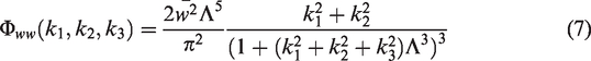
In the case of 2 D turbulent flow, at a single frequency, we consider a spectrum of vortical modes. For simplicity we consider an idealised 2 D isotropic homogeneous turbulent flow that is assumed to be frozen and convecting with a mean velocity of U. The 2 D wavenumber spectrum for the unsteady velocity component normal to the flow direction can be expressed in terms of its mean square value $\bar{w^{2}}$ and turbulence integral length scale Λ. In terms of wavenumber components (k₁, k₂) oriented in the flow-fixed reference frame, the wavenumber spectrum is of the form:

Φ_{w w} (k_{1}, k_{2}) = \int_{- \infty}^{\infty} Φ_{w w} (k_{1}, k_{2}, k_{3}) d k_{3},

(6)

where

Φ_{w w} (k_{1}, k_{2}, k_{3}) = \frac{2 \bar{w^{2}} Λ^{5}}{π^{2}} \frac{k_{1}^{2} + k_{2}^{2}}{{(1 + (k_{1}^{2} + k_{2}^{2} + k_{3}^{2}) Λ^{3})}^{3}}

(7)

and for frozen turbulence, we can write

k_{1} = ω / U

(8)

In the current CFD method, vortical modes are introduced at the inlet plane in the form of $u_{2 v} e^{i (x_{2} k_{2 v} - ω t)}$ where $k_{2 v}$ is the transverse vortical wavenumber, which can be expressed in terms of a modal index m to ensure periodicity of the form

k_{2 v} = m / R

(9)

We now use the streamwise wavenumber $k_{1} = ω / U$ and the transverse vortical wavenumber $k_{2 v} = m / R$ to determine the vortical wavenumbers in the flow-normal direction k₂ and the duct axial direction $k_{1 v}$ , the latter being necessary to deduce the streamwise velocity component $u_{1 v}$ that is consistent with the normal component $u_{2 v}$ in the divergence-free sense. Here, R is the mean radius of the cascade.

For a frozen gust, $ω = k_{1} U = \underline{k} . \underline{U}$ , where ( $\underline{k}) = [k_{1 v}, k_{2 v}]$ and ( $\underline{U}) = [U_{1}, U_{2}]$ . Resolving k₁ into its component $k_{1 v}$ and $k_{2 v}$ , leads to the following expression for the vortical wavenumber in the duct-axis direction $k_{1 v}$ ,

k_{1 v} = (ω / a - M_{2} k_{2 v}) / M_{1}

(10)

The axial velocity amplitude $u_{1 v}$ necessary in the CFD computation, may be obtained from the transverse component $u_{1 v}$ be requiring that the velocity input into the computational domain is divergence free, $\underline{k} . \underline{u} = 0$ and hence does not generate pressure by itself. This condition gives,

u_{1 v} = - u_{2 v} \frac{k_{2 v}}{k_{1 v}}

(11)

The vortical wavenumber k₂ necessary in equation (6) for the turbulence wavenumber spectra may be deduced from the transverse vortical wavenumber $k_{2 v}$ by noting $k_{2} \cos (θ) + k_{1} \sin (θ) = k_{2 v}$ and hence,

k_{2} = k_{2 v} / \cos (θ) - k_{1} \tan (θ)

(12)

Finally, the velocity amplitude $u_{2 v}$ in the duct transverse direction which forms the amplitude of the mth vortical mode can be computed from

u_{2} = u_{2 v} \cos (θ) - u_{1 v} \sin (θ)

(13)

where u₂ is the rms fluctuating velocity normal to the flow direction which can be deduced from equation (6). The vortical wave definitions (

u_{1 v}, u_{2 v}

) in (x₁,x₂) direction are imposed on the inlet boundary to solved for unsteady flow field.

To complete the analysis we note that the acoustic mode of order l is due to scattering of the vortical mode of order m and we can therefore write

l = m + B r

(14)

where B is number of blades and r is the scattering index.

In the CFD computations presented below, the radiated sound power is computed from the sum of contributions from an infinite number of incoming vortical modes m whose amplitude is determined from equation (13), where each mode is then, scattered into an infinite number of acoustic modes l.

The total radiated sound power due to a cascade of realistic aerofoils can therefore be written as sum of all cut-on acoustic modes as:

P^{\pm} (ω) = \sum_{l = l_{\min}}^{l_{\max}} P_{l}^{\pm} (ω) = \sum_{m = - \infty}^{\infty} \sum_{r = - \infty}^{\infty} P_{m, r}^{\pm} (ω)

(15)

where

P_{m, r}^{\pm}

is the radiated upstream and downstream power for an acoustic mode of

l = m + B r

The single vortical mode response due to a cascade of aerofoil is calculated using the linearised Navier-Stokes solver, HYDRA. At a specific frequency ω and a fixed vortical mode m and scattering index r the modal components of the acoustic pressure p and particle velocity $\underline{u}$ are extracted for both upstream and downstream acoustic waves at upstream and downstream locations by the use of an Eigenmode breakdown of the unsteady flow in the duct.

The total acoustic power radiated by the cascade can be computed from equation (15), where in practice, the summation over m is taken to ensure convergence of the power solution. The limits on the scattering r are restricted to the values for which the acoustics propagate. Effectively, at low frequencies, only a few vortical modes and scattering indices are required to capture all propagating acoustic modes. In this two dimensional problem, the number of propagating acoustics modes is proportional to frequency. In the current formulation, the blade response function must be computed for all combinations of vortical mode order m and scattering index r, leading to a potentially computationally intensive calculation.

In the case of a flat plate cascade, however, the blade response $R^{\pm}$ is only a function of the inter-blade phase angle $2 π m / B$ and is therefore periodic in m with period B. This periodicity problem was exploited by Cheong et al.¹⁴ to reverse the orders of summation in m and r and hence substantially improve the computational effort needed in the noise calculation to give,

P^{\pm} (ω) = \frac{2 π ρ_{0} M}{\cos θ} \sum_{m = - \infty}^{\infty} Φ_{w w} (K_{1}, k_{2}) \sum_{r = - \infty}^{\infty} | R_{r}^{\pm} (K_{1}, k_{2}) |^{2} \frac{ω R e {- a α_{r}^{\pm} + M_{1} (ω + U_{1} α_{r}^{\pm} + U_{2} β_{r})}}{| ω + U_{1} α_{r}^{\pm} + U_{2} β_{r} |^{2}}

(16)

where k₂ is the wave-number in y₂ direction expressed in vortical mode number m in circumferential (gap-wise) direction.

Broadband validation for flat plate cascades

We start with validating the flat plate model by comparing broadband sound power spectra obtained from CFD and summing over sufficient numbers of vortical modes to ensure convergence ( $\approx$ 132 in this case) with the efficient solution developed by Cheong with periodicity assumed (equation (25) in Cheong et al.¹⁴ The turbulence intensity of 2.5% and an integral length scale of $Λ = 7$ mm is used to predict the noise radiated from turbulence interactions with zero-stagger flat plate cascade. The CFD spectra plotted in Figure 3 are limited to ten discrete frequencies over the frequency range ω range of 5000 to 40000 and compared to the LINSUB solution with a much finer frequency resolution is around 1 dB. This difference is due to numerical issues relating to convergence of solution at the frequencies for which there are acoustical modes close to cut-on.

Figure 3.

Overall radiated power across various frequencies at incoming turbulence intensity, $T I = 2.5 %$ , and integral length scale $Λ = 7$ mm. (a) Turbulence length scales. (b) Turbulent intensity

The numerical CFD approach described above and validated for a flat plate cascade is now used to investigate the effect on broadband noise due to changes in aerofoil geometry such as blade thickness, noise radius. The current numerical simulations are performed on 5 different 2 D section along the span. In all these simulations periodocity property of the blade response is used, hence, only modes between 0 and B are summed to estimate the modal powers.¹⁶ The knowledge of the turbulence characteristics is important to estimate the $Φ_{w w}$ and used in equation (16) by assuming homogeneous turbulence.

Turbulence extraction from rotor wake

RANS simulations are performed on the ACAT Rotor geometry with the corresponding baseline OGV and ESS blades. Approach conditions were simulated at the operating point of 3672 rpm. The mass flow rate for the core and bypass flow at the Approach conditions are 7.46 and 46.76 kg/s respectively.

A single blade passage is considered in this analysis to extract the wake characteristics at the downstream of the rotor. The mesh is generated using the Rolls-Royce in-house software PADRAM. An H-O-H mesh topology is used to grid the rotor, OGV and ESS passages. Approximately 6.5 million nodes are used to mesh the Rotor, OGV and ESS passage. The boundary layer is fully resolved on the blades ( $y^{+} < 1$ ). Compared to the rotor grid, a slightly different meshing strategy is employed to create the inlet block to the OGV computational grid. In order to take into account the possibility of large variations in the stator sweep, a hybrid approach is used in which the inlet block to the OGV domain is unstructured on the azimuthal planes.

Subsonic conditions are imposed on the inlet and outlet boundary surfaces of the domain. The outlet pressure is interactively modified to obtain the correct pressure ratio and mass flow rate such that the performance of the rotor falls on the working line. The k−ω turbulence model and a mixing-plane between the rotor and stator blocks are used in the simulations.

We now extract the turbulence characteristics which will be later used to estimate the velocity two-point cross-spectra. The circumferentially-averaged turbulence length scales and turbulence intensities are estimated from these RANS solutions. The turbulence length scales are estimated from the half-wake width δ_w using the empirical relationship, $0.21 δ_{w}$ and the turbulence intensity is estimated from turbulent kinetic energy k.

Figure 4 shows the variation of Turbulence length scales and Turbulence intensity along the radius at approach.

Figure 4.

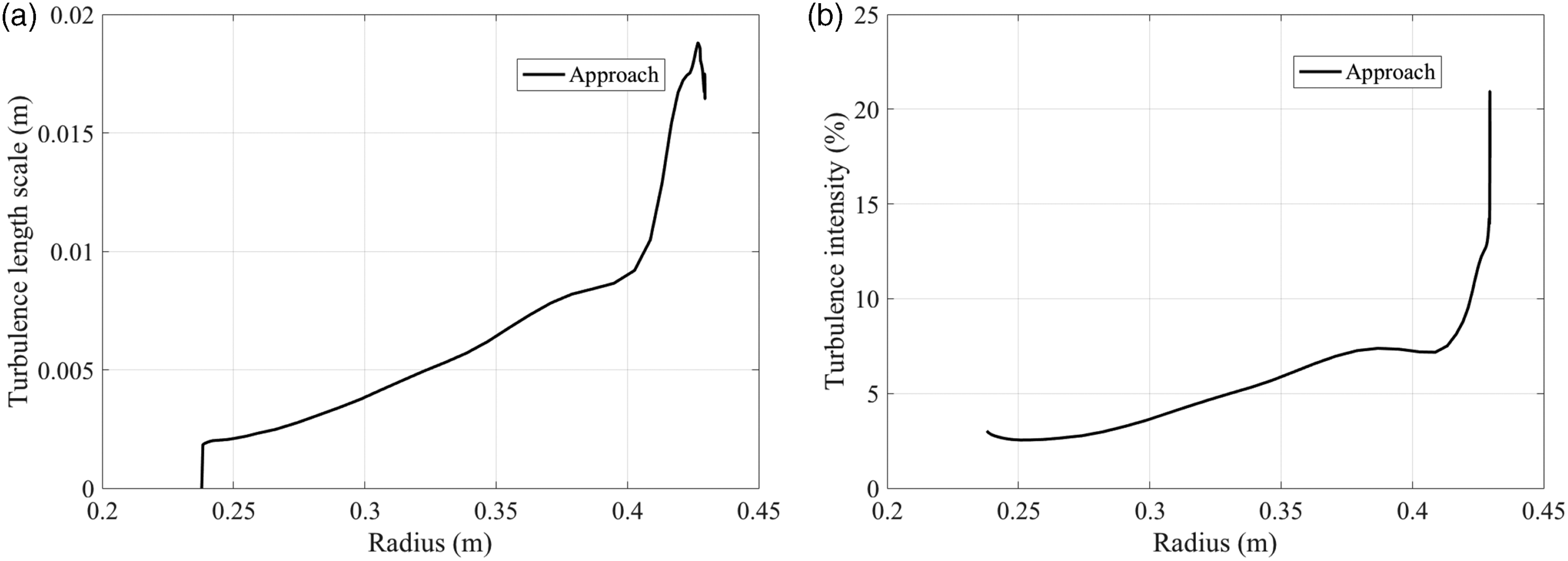
Extracted circumferentially average turbulence characteristics at upstream of mixing plane.

To estimate the total radiated noise for complete OGV, 5 different span location 10, 25, 50, 75 and 90% are considered in this study and turbulence characteristics are interpolated to desired location.

Bayesian optimisation framework

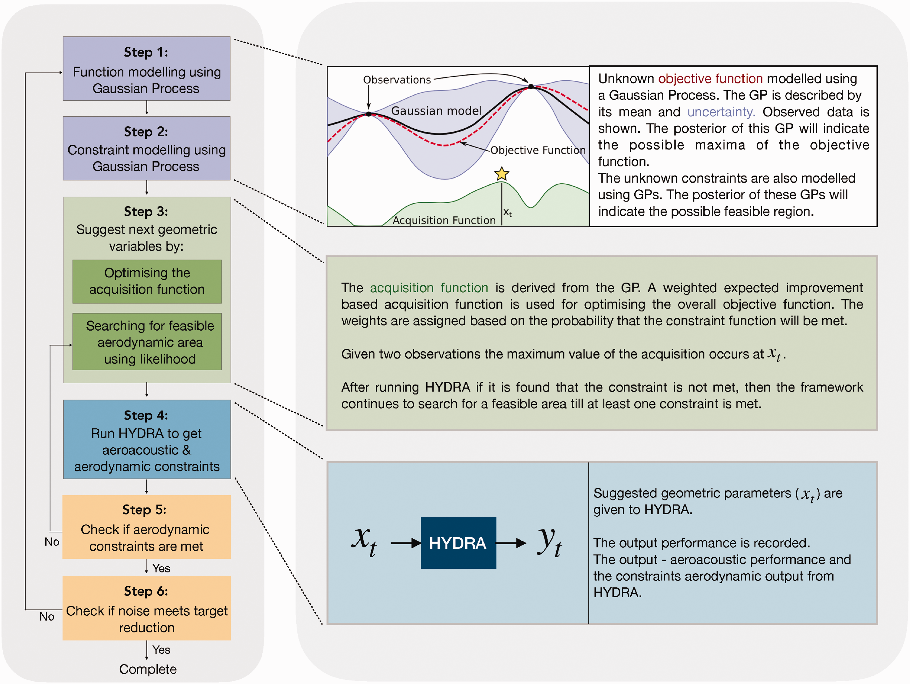
In this section, we introduce the Bayesian optimisation framework and briefly describe its essential building blocks followed by an algorithm proposed by Gelbart et al.³⁶ that applies this general framework with constraints.

Bayesian optimisation is an iterative approach of sampling data and updating the model search space that consists of two main components: The Gaussian process and the acquisition function. The Gaussian process (GP)³² is used to model the unknown objective function. The GP can be completely described by its mean and covariance and it captures our beliefs and uncertainties about the objection function. As more data is available and the GP is updated and the uncertainty around observed data and their neighbourhood reduces. Given some data, the properties of GP allow us to compute the predictive mean and predictive variance at all points in the domain. The GP however cannot be used directly for optimisation, as the function is expensive to sample and can potentially shoot up the experimental cost. Instead a surrogate function, which is cheaper to compute, called as an acquisition function is derived from the GP. The acquisition function implements a strategy to guide the search for the optima.

Two extreme strategies of conducting a search for the optima are exploitation and exploration. Exploitation is a greedy search around a likely minima. Here the GP mean will be high and thus we are more likely to get an improvement over the current optima. Exploration on the other hand is a search in regions where variance of GP is high. When such points are recommended the resulting experiment may not necessarily improve the optima, but this encourages reduction of uncertainty of GP where no points have been sampled and avoids being stuck in local optima and also gives us confidence in the convergence over time. Generally, the acquisition functions are designed to combine these two strategies using the posterior mean and variance of the GP. Maximising the acquisition function at any given iteration allows us to choose the next point at which the function should be evaluated experimentally. This point brings the search for the optima one step closer.

Gaussian process

Just as a Gaussian distribution is a distribution over a random variable, completely specified by its mean and covariance, a Gaussian process (GP)³² is a distribution over functions, completely specified by its mean function, m(x) and covariance function, $k (x, x')$ :

f (x) \sim G P (m (x), k (x, x'))

(17)

A common method to model an unknown function f(x) is by using a Gaussian process with a zero mean function as a prior³³ that is, $f (x) \sim G P (0, K (x, x'))$ . Using an observation model of $y = f (x) + ϵ$ , where $ϵ \sim N (0, σ_{noise}^{2})$ , and denoting available data $D = {x_{i}, y_{i}}_{i = 1}^{t}$ one can derive the predictive distribution as:

P (f_{t + 1} | D_{1 : t}, x) = N (μ_{t + 1} (x), σ_{t + 1}^{2} (x))

(18)

where,

μ_{t + 1} (x) = k^{T} {[K + σ_{noise}^{2} I]}^{- 1} y_{1 : t}

(19)

σ_{t + 1} (x) = k (x, x) - k^{T} {[K + σ_{noise}^{2} I]}^{- 1} k

(20)

where,

k = [k (x, x_{1}), k (x, x_{2}), \dots, k (x, x_{t})]

, the kernel matrix

[K_{i j}] = k (x_{i}, x_{j}) \forall i, j \in 1, \dots, t

Kernel function

The kernel or the covariance function is a crucial component for Gaussian process prediction, as it encodes the assumptions about the objective function $f (x)$ . The covariance between the sample points in the design space determines the smoothness of the functions which are most likely given by the GP. The squared exponential kernel is one of the most popular kernel function. It is known to be the best function to use when there is little known about the objective function. It is defined as

k_{S E} (x_{i}, x_{j}) = \exp (- \frac{1}{2 θ^{2}} | | x_{i} - x_{j} | |^{2})

(21)

where the kernel length-scale θ affects the smoothness of the objective function – a larger value means a smoother function.³²

Another kernel which has been used in this paper is the Matérn kernel. It is also a statistical covariance that only depends on the distance between the points. It is defined as follows:

k_{Matern} (x_{i}, x_{j}) = \frac{1}{2^{ς - 1} Γ (ς)} {(2 \sqrt{ς} | | x_{i} - x_{j} | |)}^{ς} H_{ς} (2 \sqrt{ς} | | x_{i} - x_{j} | |)

(22)

where

Γ (\cdot)

and

H_{ς} (\cdot)

are the Gamma function and the Bessel function of order

ς = 5 / 2

³²

Acquisition function

Two of the acquisition functions that the algorithm in this paper are based on are Expected Improvement (EI) and Upper Confidence Bound (UCB). They are given as follows:

EI (x) = {\begin{array}{l} (μ (x) - f (x^{+})) Φ (Z) + σ (x) ϕ (Z) σ (x) > 0 \\ 0 σ (x) = 0 \end{array}

(23)

where

Z = \frac{μ (x) - f (x^{+})}{σ (x)}, f (x^{+})

is the current maxima.

Φ (Z)

and

ϕ (Z)

are the normal cumulative distribution function and the normal probability distribution function of standard normal distribution²¹

GP-UCB (x) = μ (x) + \sqrt{v β_{t}} σ (x)

(24)

where, recommended values for v and the confidence parameter are v = 1 and

β_{t} = 2 l o g (t^{d / 2 + 2} π^{2} / 3 δ)

respectively, d represents the dimensionality of the data, t is the iteration number, and

δ \in (0, 1)

³⁴

General bayesian optimisation process with constraints

Consider our main objective is to optimise aeroacoustic performance constrained by a target aerodynamic performance. We note that the aerodynamic constraints are not known beforehand. One must run HYDRA simulations to extract both aerodynamic and aeroacoustics performance at cruise and approach conditions. Hence, in this scenario both the objective and constraint functions are unknown and expensive to compute. The framework must together handle the optimisation of objective function (aeroacoustic) and search for feasible region that meets constraints (aerodynamic). In this section, we look at incorporating aerodynamic constraints into the previously presented general framework as proposed by Gelbart et al.³⁶ which provides a solution for Bayesian optimisation for unknown constraints.

Let us assume that the objective and constraint functions are mutually independent as the inherent processes corresponding to each result from separate black-box functions. This allows us to model aerodynamic performance using a separate GP and estimate the likelihood that its requirements are met using the predictive likelihood.

Suppose that $C_{l} (x)$ is a boolean function which indicates whether the condition l is satisfied or not. Then the probability that the constraint will be met is given as $Pr (C_{l} (x)) \geq 1 - δ_{l}$ for some user defined confidence δ. At the solution of the optimisation problem, we expect all l constraints to be satisfied. The optimisation problem is given by

x^{*} = {argmax}_{x \in X} f (x) s . t . \forall k Pr (C_{l} (x)) \geq 1 - δ_{l}

(25)

Consider a latent real valued function $g_{l} (x)$ and suppose we can define it such that the constraint function $C_{l} (x)$ will be met only when $g_{l} (x) \geq 0$ . We can model $g_{l} (x)$ using a Gaussian Process and $Pr (C_{l} (x)) = Pr (g_{l} (x) \geq 0)$ can be computed using the predictive mean and variance of the GP at x.

In this model, the acquisition function has been modified since expected improvement will be stalled when constraints are not met. A weighted constraint function based on Expected Improvement (EI) is used which is defined as below:

α (x) = E I (x) P r (C (x)) = E I (x) \prod_{l = 1}^{L} P r (C_{l} (x))

(26)

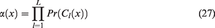
When at least one constraint is not satisfied, the above acquisition function cannot be calculated. Then BO is forced to keep searching for the feasible area before it returns to optimisation. When this happens the acquisition function for searching feasible area is given as,

α (x) = \prod_{l = 1}^{L} P r (C_{l} (x))

(27)

The optimisation process is summarised in Figure 5 and takes places in 6 steps. Step 1 involves the function modelling using GP. Step 2 involves constraint function modelling using GP. Step 3 optimises the acquisition function to suggest the next geometric variables, where constraint are likely to be met. At step 4 these design parameters are given to HYDRA and the new aeroacoustic and aerodynamic performance values are collected. Step 5 checks whether constraints are met. Within this step if the constraints are not met, then BO goes back to step 3 and keeps searching the constraint function space till a feasible area is found. Finally the next design parameters are recommended. If the constraints are met then step 6 checks if the aeroacoustic performance meets the desired target and the process is stopped. If the target is not achieved the next iteration begins from step 1.

Figure 5.

OGV optimisation process with constraints (Adapted from Li et al.³⁵). (a) upstream power. (b) downstream power

Results

Conventional approach

In this section, we first perform conventional grid search based optimisation. The primary goal is to optimise the OGV for noise at approach condition with a limited penalty on aerodynamics at cruise condition. Linear HYDRA simulations are performed at 6 different frequencies of 1 BPF to 6 BPF for the DLR baseline geometry at 5 different spanwise sections 10, 25, 50, 75 and 90% height locations and summarised in Table 1. Appropiate turbulence length scales and intensity extracted from the fan RANS simulations at approach conditions are used for the predictions. Predicted upstream and downstream values are A-weighted, based on the frequency of interest at full scale. For example, at 1BPF, 250 Hz dBA correction is applied and so on.

Table 1.

Radiated upstream and downstream power (dBA) for five different span locations at approach condition.

	1BPF		2BPF		3BPF		4BPF		5BPF		6BPF		Overall
Span	US	DS	US	DS	US	DS	US	DS	US	DS	US	DS	US	DS
10%	67.37	67.11	70.94	71.51	72.74	73.87	70.69	72.06	68.28	75.67	68.64	73.97	77.95	80.85
25%	75.55	74.13	78.88	78.82	78.69	80.39	76.51	82.15	75.07	80.02	74.14	76.82	84.62	87.20
50%	78.60	79.89	83.14	83.66	81.88	83.47	79.01	84.11	78.12	80.75	73.77	77.20	87.79	89.92
75%	81.65	79.63	84.07	84.85	78.21	85.40	78.46	82.24	75.54	78.39	71.76	74.87	87.70	90.05
90%	82.81	82.41	82.88	82.91	78.59	81.76	74.73	76.32	69.57	72.67	66.26	70.41	86.99	87.72

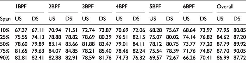
It is clear from Table 1 that the dominant section of OGV is mid-span (50%) and 75% height. Even though the velocities are dominant at the hub, the turbulence intensity and length scales are observed to be dominant at the tip. Hence, the maximum radiated noise is observed at midspan suggesting $U^{3} u^{2}$ as the key parameter for radiated noise. We now consider mid-span section and perform the low-noise design optimisation.

Linear HYDRA simulations are performed at 6 different frequencies of 1BPF to 6 BPF for all the 54 different aerofoils of varying thickness and nose radius. At each frequency, a total of 22 azimuthal modes are computed and summed up to achieve upstream and downstream radiated power due to cascade of aerofoils. Here, we assume the periodicity condition is applicable in the OGV response, in order to calculate the broadband noise due to impinging turbulence of integral length scale of 5.5 mm and intensity of 5%. Change in overall radiated power contour relative to baseline OGV are plotted in Figure 6(a) and (b). It is very evident for the figure that with the parameters chosen i.e., thickness and nose radius we can only reduce up to 0.8 dB, which is with in numerical uncertainty.

Figure 6.

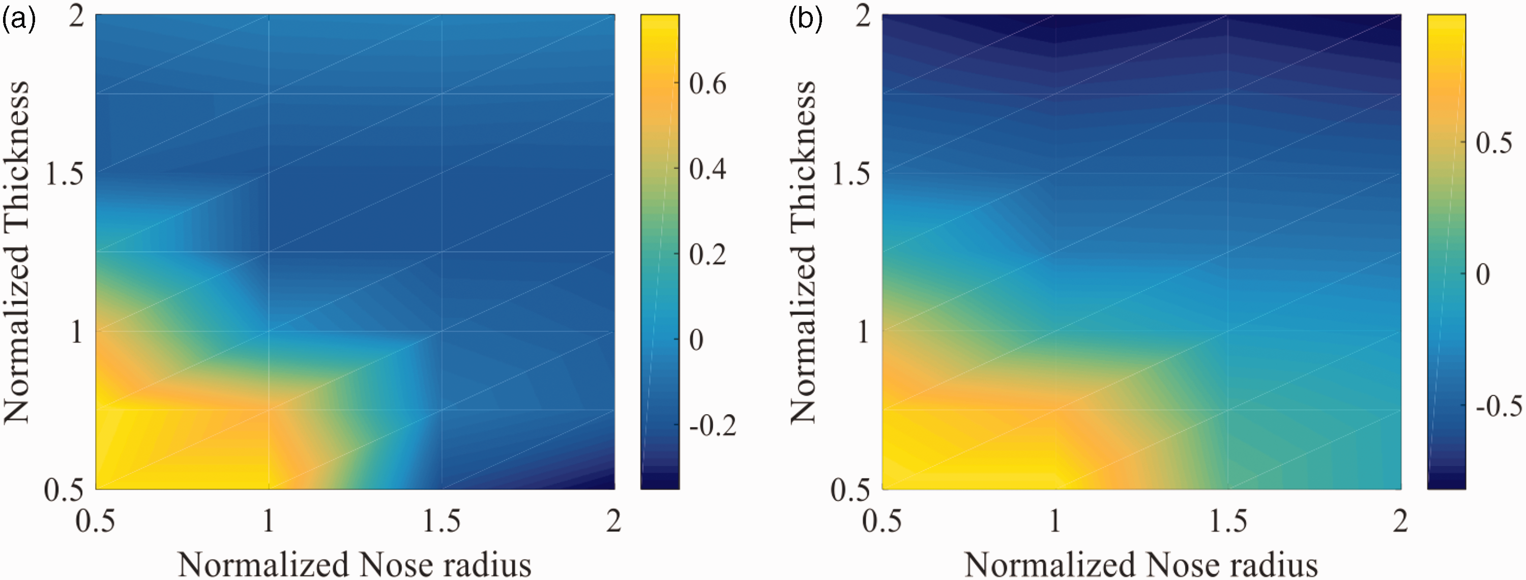
Change in overall sound power (1-6BPF) due to changes in 2 D geometry configurations at mid-span. (a) Pressure loss in %. (b) Flow exit angle (degrees)

The results are consistent with literature that blunt nose radius or thicker aerofoils produce less radiated noise than compared to sharp and thin aerofoils. This shows our approach captures the small geometric changes on the radiated power. The change in noise is also consistent with frequency. We see greater changes in radiated power at higher frequencies than compared to low frequencies. This is consistent with authors previous study;^16,17,20 suggesting ft/U is the key parameter for noise reductions.

RANS simulations are performed on the above mentioned 54 aerofoil designs of varying thickness and nose radius. Subsonic inlet and outlet conditions are imposed on the inlet and outlet boundary surfaces of the domain. Outlet BC of the Fan domain at cruise condition are imposed at the inlet boundary of OGV domain (mid-span). The boundary conditions are fixed for all different geometric configurations. The aerodynamic performance parameters such as pressure loss across the OGV and the flow exit angle are calculated and plotted for various aerofoil geometries in Figure 7. An optimum around normalised thickness of 1 is observed from the pressure loss contours as seem from Figure 7(a), this is consistent with literature as OGV are designed for aerodynamics. With the increase in aerofoil thickness we observed drastic increase in pressure loss which makes thicker aerofoils non-favourable for aerodynamics. Flow exit angle is one of the important criteria but the change in flow exit angle is within $\pm^{4}$ . This parameter is not as important when compared to pressure loss. Hence, the aero factor considered in this study is given by

Aero = 0.9 P + 0.1 θ

(28)

where P is the pressure loss in % and θ is flow exit angle.

Figure 7.

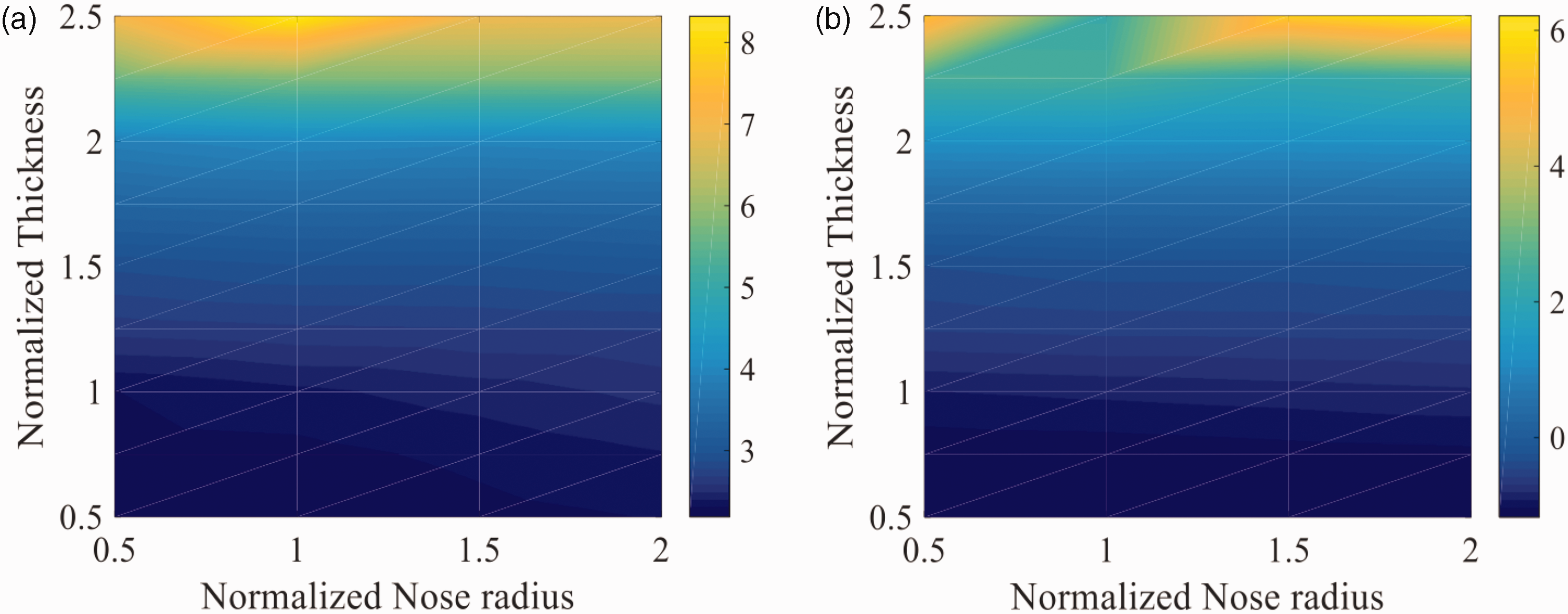
Aerodynamics performance evaluation for different geometries.

We now combine both aerodynamic and aeroacoustic performance to achieve the optimised low-noise OGV mid-section. Figure 8 shows the variation of overall downstream sound power reductions versus aero factor for different aerofoil configurations. Note that the overall sound power is calculated using 1–6 BPF and aero factor is calculated using equation (28). It is very clear from the results, that to achieve 0.5 dB noise reduction the penalty on the aerodynamic is 33% poorer than baseline aerofoil. Hence, the geometry changes such as thickness and nose radius can’t reduce broadband noise without effecting aerodynamic performance. Other Input and output parameters listed in above section are not considered because their influence on noise is negligible from previously available literature. To achieve this conclusion, we need to run at least 54 geometries and for each geometry the number of simulations are function of number of frequencies and number of azimuthal modes. The further part of the paper describes the use of Bayesian Optimisation to reduce the computational cost of the simulation.

Figure 8.

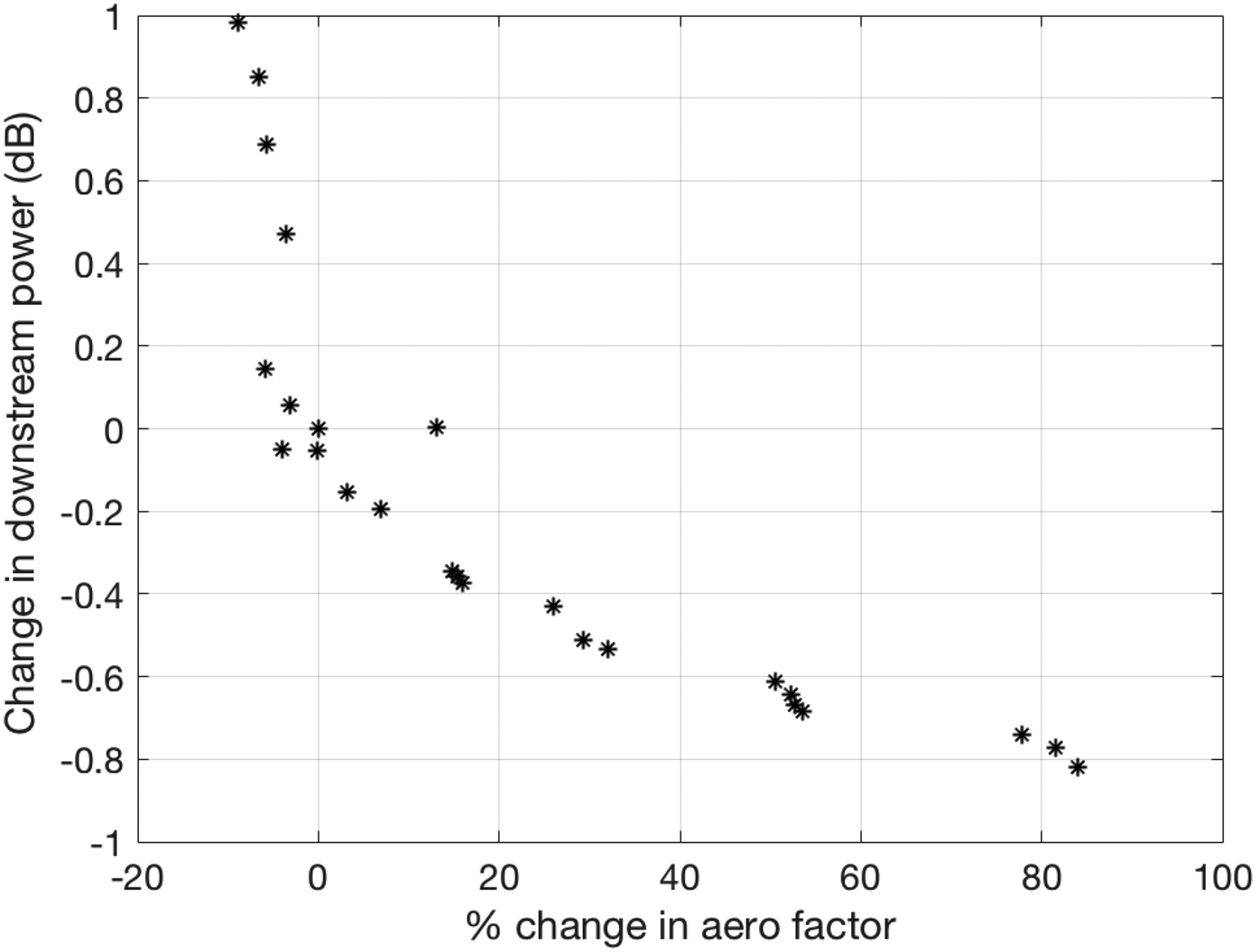
Pareto front for aerodynamic and aeroacoustic performance. (a) between 20.0 and 30.0%. (b) Less than 30%

Bayesian optimisation

In this experiment our goal is to demonstrate that Bayesian optimisation (BO) is cost effective approach to design low-noise OGV with aerodynamic constraints. We apply the Bayesian optimisation with unknown constraints algorithm proposed by Gelbart et al.³⁶ as explained in Figure 5. Here, the objective function, which is unknown is modelled as a measure of the aeroacoustic performance characteristics with respect to input parameters. We run Bayesian optimisation on the discretised data as shown in Figure 6. Here the constraint function is percentage change in aero factor which is estimated by equation (28).

Figure 9 shows the results of two experiments, where the aerodynamic constraint is specified by upper and lower bounds (feasible area). The dots represent the points outside the feasible area, which indicate that the constraint was not met and Bayesian optimisation fell back to searching for a feasible area at these steps (transition from step 5 to step 3 in Figure 5). The triangular points indicate the region where constraints were met. Finally, the red triangle indicates the minima found by Bayesian optimisation.

Figure 9.

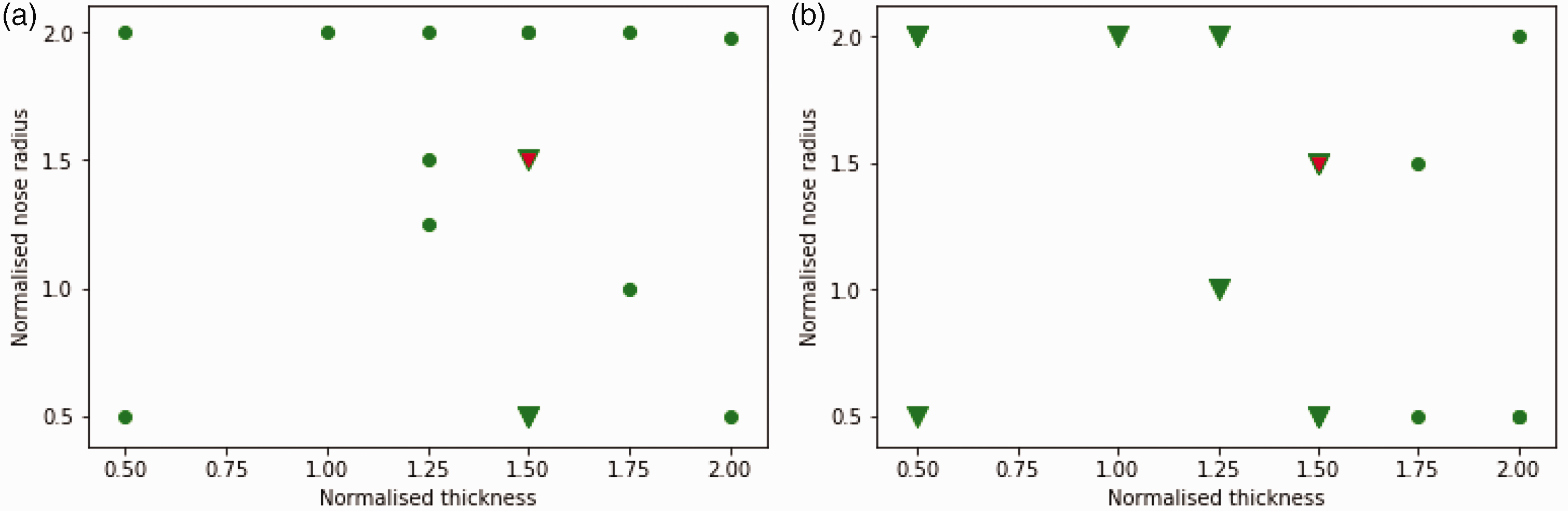
Optimisation of aero-acoustic performance by measuring the pressure loss given that the aerodynamic performance.

In the first experiment we constrained the aerodynamic performance to be between 20% to 30% of the change in aero factor. BO was started with three initially points and ran for 10 iterations. The optima was found in 7 iterations within a grid of 56 points. From Figure 8, the feasible area for this constraint consists of only 2 grid points. This is consistent with the BO optimisation approach as seen in Figure 9(a) (as shown in triangles). As we know blunt aerofoils produces less noise, the case with larger normalised nose radius is observed to be minima.

In the second experiment we constrained the aerodynamic performance to less than 30% change in aero factor. In this experiment Bayesian optimisation finds the optima that meets the constraint in 10 iterations within the same grid of 56 points. From Figure 8, the feasible area for this constraint is much larger which is consistent with triangles as shown in Figure 9(b) which is obtained using BO. The optima identified by both the experiments is the same which shows the robustness of the BO approach.

From these experiments, we have demonstrated the effectiveness of Bayesian optimisation approach for designing low-noise OGV with aerodynamic constraints. The aerodynamic constraints can be specified either as a range or as an upper/lower bound. Hence, the proposed BO approach save lot of computational cost (almost 1/3rd) as compared to a conventional grid search especially when the input variables are greater.

Conclusion

Optimising OGV geometry for aerodynamic and aeroacoustic benefits is a fairly expensive process. While the RANS simulations are less expensive, noise calculations for each geometry in the design space is increased by 40 folds for each frequency. In the present work, with the goal to reduce the computational cost we try to control the design parameters of the blade (nose radius and thickness) to achieve minimum aerodynamic penalty. Bayesian optimisation framework has been applied to reach the optimum value with significantly fewer number of evaluations. It was successfully demonstrated that Bayesian Optimisation is a powerful approach which drastically saves the computation time of the optimisation routine for aeroacoustics performance with aerodynamic constraints. This paper shows that to achieve noise reductions of 0.5 dB the penalty on the aerodynamic performance of 33% is observed compared to baseline aerofoil. Hence, the geometry changes such as thickness and nose radius can’t reduce broadband noise without effecting aerodynamic performance. 3 D geometric changes such as serrations or slits on OGVs might be a way forward to reduce the turbulence-cascade interaction noise.

Footnotes

Acknowledgements

The authors would also like to thanks Rolls-Royce for technical support. Special thanks to Prof. Phillip Joseph and Mr. John Coupland for his constant support all along this work. Thanks to Dr. Anuroopa kalyan for proof reading the paper.

Declaration of conflicting interests

The author(s) declared no potential conflicts of interest with respect to the research, authorship, and/or publication of this article.

Funding

The author(s) disclosed receipt of the following financial support for the research, authorship, and/or publication of this article: The presented work was conducted in the frame of the project TurboNoiseBB, which has received funding from the European Union’s Horizon 2020 research and innovation program under grant agreement No. 690714. The authors also gratefully acknowledge the support of the Innovate UK Aerospace Technology Institute through the funded research program ACAPELLA (Advanced Capability for Prediction of Engine Level Acoustics, ref.113086].

ORCID iD

Paruchuri Chaitanya

References

Lane

Friedman

Unsteady aerodynamics of vortical flows: early and recent developments. Tech. rep. NACA-TN-4136, 1958.

Whitehead

Bending flutter of unstalled cascade blades at finite deflection. Tech. rep., Reports and Memoranda R. & M. No. 3386, Ministry of Aviation, Aeronautical Research Council, London, 1965.

Kaji

Okazaki

Cascade flutter in compressible flow. Jsmet 1972; 38: 1023–1033.

Smith

Discrete frequency sound generation in axial flow turbomachines. Aeronaut Res Council Rep Memoranda 1972; 3709: 1--56.

Whitehead

AGARD manual on aeroelasticity in axial-flow turbomachines. Volume 1. Unsteady turbomachinery aerodynamics. Chaps. In: Classical two-dimensional methods (eds MF Platzer and FO Carta), 1987, pp. 3.1–3.30. Loughton, EIssex: Specialised Printing Services Limited.

Mani

Horvay

Sound transmission through blade rows. J Sound Vibr 1970; 12: 59–83.

Peake

The interaction between a high-frequency gust and a blade row. J Fluid Mech 1992; 241: 261–289.

Peake

The scattering of vorticity waves by an infinite cascade of flat plates in subsonic flow. Wave Motion 1993; 18: 255–271. Vol.

Peake

Kerschen

Influence of mean loading on noise generated by the interaction of gust with plate cascade: upstream radiation. J Fluid Mech 1997; 347: 315–346.

10.

Evers

Peake

On sound generation by the interaction between turbulence and a cascade of airfoils with non-uniform mean flow. J Fluid Mech 2002; 463: 25–52.

11.

Hanson

Horan

Turbulence/cascade interaction: spectra of inflow, cascade response and noise. In: Proceedings of the 4th AIAA/CEAS aeroacoustics conference, Toulouse, France, 2--4 June 1998, No. 1998-2319.

12.

Glegg

Broadband Fan noise generated by small turbulence length scale. Tech. rep., 1998.

13.

Glegg

The response of a swept blade row to a three-dimensional gust. J Sound Vibr 1999; 227: 29–64.

14.

Cheong

Joseph

Lee

High frequency formulation for the acoustic power spectrum due to cascade-turbulence interaction. J Acoust Soc Am 2006; 119: 108–122.

15.

Polacsek

Clair

Garrec

, et al. Numerical predictions of turbulence/cascade-interaction noise using computational aeroacoustics with a stochastic model. AIAA J 2015; 53: 3551–3566.

16.

Chaitanya

Coupland

Joseph

Aerofoil geometry effects on turbulence interaction noise in cascades. In: 22nd AIAA/CEAS aeroacoustics conference, Lyon, France, 30 May--1 June 2016, No. 2016-2738.

17.

Chaitanya

Aerofoil geometry effects on turbulence interaction noise. PhD thesis, University of Southampton, ISVR, 2017.

18.

Hainaut

Prediction and analysis of broadband interaction noise using synthetic turbulence. PhD thesis, University of Southampton, ISVR, 2017.

19.

Gea-Aguilera

Gill

Zhang

On the effects of fan wake modelling and vane design on cascade noise. J Sound Vibr 2019; 459: 114859.

20.

Chaitanya

Gill

Narayanan

, et al. Aerofoil geometry effects on turbulence interaction noise. In: 21st AIAA/CEAS aeroacoustics conference, Dallas, TX, 22-26 June 2015. No. 2015-2830.

21.

Jones

Schonlau

Welch

WJ.

Efficient global optimization of expensive black-box functions. J Global Optimization 1998; 13: 455–492.

22.

Shahriari

Swersky

Wang

, et al. Taking the human out of the loop: a review of Bayesian optimization. Proc IEEE 2016; 104: 148–175.

23.

Chaitanya

Vellanki

Kalyan

, et al. Low-noise OGV design for broadband noise using Bayesian optimisation. In: 25th AIAA/CEAS aeroacoustics conference Delft, The Netherlands, 20-23 May 2019, No. 2019–2489.

24.

Frazier

Wang

Bayesian optimization for materials design. In: Information science for materials discovery and design. Berlin: Springer, 2016, pp.45–75.

25.

Ueno

Rhone

Hou

, et al. COMBO: an efficient Bayesian optimization library for materials science. Mater Discovery 2016; 4: 18–21.

26.

Lorenz

Monti

Violante

, et al. The automatic neuroscientist: a framework for optimizing experimental design with closed-loop real-time fMRI. NeuroImage 2016; 129: 320–334. Vol.

27.

Cully

Clune

Tarapore

, et al. Robots that can adapt like animals. Nature 2015; 521: 503–507.

28.

Moinier

Algorithm developments for an unstructured viscous flow solver . PhD thesis, Oxford University, UK, 1999.

29.

Campobasso

Duta

Giles

MB.

Effects of flow instabilities on the linear analysis of turbomachinery aeroelasticity. J Propul Power 2003; 19: 693–703.

30.

Moinier

Giles

MB.

Eigenmode analysis for turbomachinery applications. J Propulsion Power 2005; 21: 973–978..

31.

Moinier

Giles

Coupland

Three-dimensional non-reflecting boundary conditions for swirling flows in turbomachinery. J Propulsion Power 2007; 23: 981–986.

32.

Rasmussen CE and Williams CKI. Gaussian Processes for Machine Learning. The MIT Press, 2006. ISBN 0-262-18253-X.

33.

Brochu

Cora

de Freitas

A tutorial on Bayesian optimization of expensive cost functions, with application to active user modeling and hierarchical reinforcement learning. arXiv:1012.2599, No. UBC TR-2009-023 and arXiv:1012.2599, 2010.

34.

Srinivas

Krause

Kakade

, et al. Gaussian process optimization in the bandit setting: no regret and experimental design. In: ICML'10: Proceedings of the 27th international conference on machine learning, June 2010, pp. 1015–1022. United States: Omnipress.

35.

de Celis Leal

Rana

, et al. Rapid Bayesian optimisation for synthesis of short polymer fiber materials. Sci Rep 2017; 7: 5683.

36.

Gelbart

Snoek

Adams

RP.

Bayesian optimization with unknown constraints. In: UAI'14: Proceedings of the thirtieth conference on uncertainty in artificial intelligence, July 2014, pp. 250?259. United States: AUAI Press.

Bayesian optimisation for low-noise aerofoil design with aerodynamic constraints

Abstract

Keywords

Introduction

Problem definition

Flow chart

Input and output parameters

Numerical approach

Steady flow simulations

Linear unsteady CFD simulations

Mesh generation and boundary conditions for unsteady simulations

Turbulence synthesis

Fourier description of the radiated sound power from 2 D aerofoil cascades

Broadband validation for flat plate cascades

Turbulence extraction from rotor wake

Bayesian optimisation framework

Gaussian process

Kernel function

Acquisition function

General bayesian optimisation process with constraints

Results

Conventional approach

Bayesian optimisation

Conclusion

Footnotes

Acknowledgements

Declaration of conflicting interests

Funding

ORCID iD

References