Impedance modelling of acoustically treated circumferential grooves for over-tip-rotor fan noise suppression

Abstract

Experimental investigation of Over-Tip-Rotor circumferential groove liners has shown potential for fan noise suppression in turbofan engines whilst providing minimal penalty in fan aerodynamic performance. The validation of Over-Tip-Rotor liner analytical prediction models against published experimental data requires the modelling of an equivalent impedance for such acoustic treatments. This paper describes the formulation of two analytical groove impedance models as semi-locally reacting liners, that is locally reacting in the axial direction and non-locally reacting in the azimuthal direction. The models are cross-verified by comparison with high-order FEM simulations, and applied to a simplified Over-Tip-Rotor configuration consisting of multiple grooves excited by a monopole point source located close to the grooved surface.

Introduction

Over-Tip-Rotor (OTR) liners embedded within the fan case have been investigated over recent decades as a technology with the potential to provide additional suppression of fan noise in turbofan engines. These studies have also assessed the effect of OTR liners on the aerodynamic performance of the fan. The use of circumferential grooves in OTR liners has shown a reduction in the aerodynamic performance penalty of the fan attributed to a decrease of the dynamic pressure on the acoustic treatment.^1,2 This led to liner designs which consist of a casing of circumferential grooves with and without absorbing elements. Acoustic test results from a single stage axial compressor at NASA-GRC with and without OTR liners has shown a net PWL insertion loss benefit of 2.5–3.5 dB for forward propagating modes. ³

The work described here has been developed as part of a study at the ISVR to contribute to the understanding of the acoustic attenuation of OTR liners by using analytical models based on monopole and dipole Green's functions for lined cylindrical ducts. The analytical prediction models are being assessed against the experimental data from the OTR circumferential groove array tested in the NASA-GRC W-8 fan rig. ³ An analytical impedance model equivalent to the acoustically treated circumferential grooves used in the experiments is required as an input to our OTR prediction models. ⁴

The modelled OTR fan case configurations consist of circumferential grooves extending over an axial length equal to the axial projection of the fan chord. The grooves are formed of upper and lower parts, this arrangement is illustrated in Figure 1(b) where the lower and upper parts of the groove are labelled ① and ② respectively. The upper part ② is open at the top and terminated at the base with a ‘septum’. Below the septum the lower part of the groove ① is partitioned azimuthally and can also be filled with acoustically absorbing material. This means that the upper portion of the groove in which the propagation is permitted in the azimuthal direction is bounded by a porous interface to the lower portion which is truly locally reacting due to the azimuthal partitions. The particular case of a hard ‘septum’ is also considered, in which part ② is terminated by a hard wall and therefore part ① is not modelled, as illustrated in Figure 1(a). The case where the septum is acoustically hard can be considered as a particular case of the annular partitioned bulk-reacting liner model published by Rienstra, ⁵ where the bulk properties match those of air, or as a limiting case of the spiralling non-locally reacting liner of Sijtsma et al., ⁶ when the spiral angle is set to zero.

Figure 1.

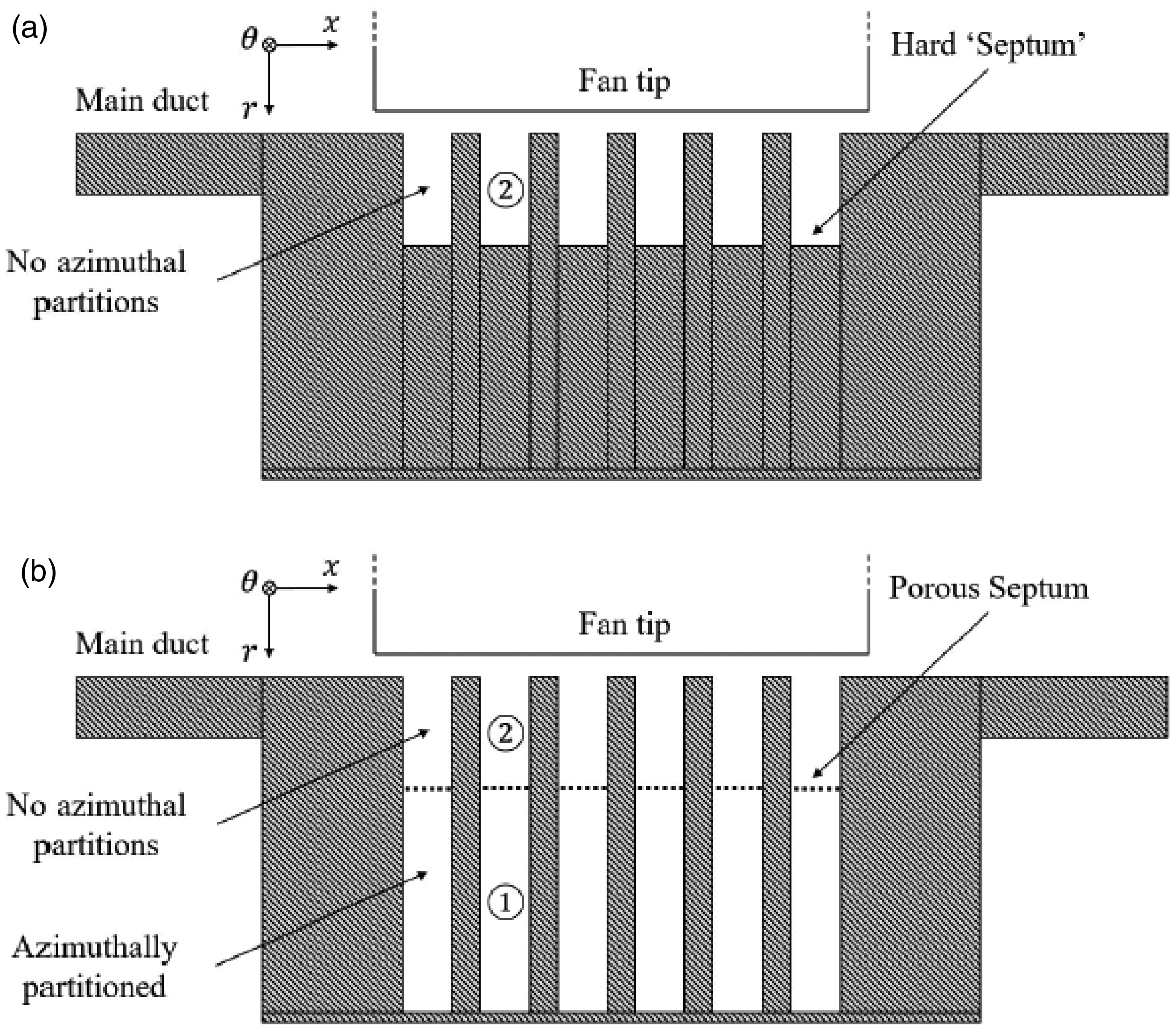
OTR circumferential groove array as tested in NASA W-8 fan rig. (a) Hard ‘septum’. (b) Porous ‘septum’.

This paper details the formulation and underpinning assumptions of two analytical groove impedance models as semi-locally reacting liners. The formulation presented here has been outlined in a previous article by the authors, ⁴ but is covered here in more complete detail and includes a verification against high-order FEM simulations performed with the commercial software Simcenter 3 D Acoustics. ⁷ A number of numerical case studies are presented to demonstrate the acoustic response of the groove to incident duct modes. Single and multiple groove configurations are used for modal solutions in the airway and for the W-8 groove geometry excited by a point source. Numerical results for the pressure and radial particle velocity are evaluated at the interface between the groove/s and the main duct, and these are used to obtain an equivalent impedance which is directly comparable to that obtained from the analytical models.

Formulation of the analytical models for the groove liner impedance

The analytical impedance models presented here aim at characterising the acoustic behaviour of the OTR circumferential groove array tested in the NASA W-8 fan rig. In particular, two configurations are considered taken directly from the experimental datasets.³ Both treatments consist of circumferential grooves that cover the axial projection of the fan chord, with the base of the upper portion of the grooves terminated by a hard or porous septum as indicated in Figure 1. A photograph of the actual treatment tested in the W-8 rig is shown in Figure 2(a). Note that the lower partitioned portion of the groove is filled in this case with metal foam.

Figure 2.

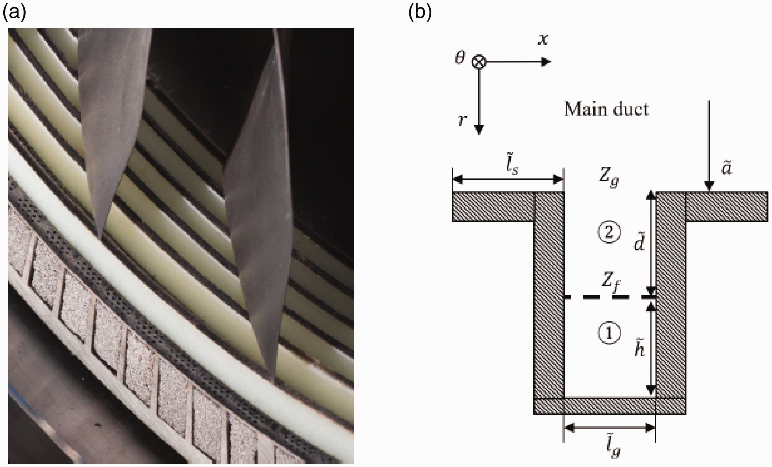
OTR fan case liner: (a) View of the OTR fan case liner installed in the NASA W-8 fan rig³ and (b) dimensional diagram of the problem and nomenclature.

A dimensional diagram of a single groove and the nomenclature used in the derivation of the equivalent acoustic impedance is shown in Figure 2(b). Regions ① and ② refer to the portions of the groove below and above the septum, of depth $\tilde{d}$ and $\tilde{h}$ respectively. ${\tilde{l}}_g$ and ${\tilde{l}}_s$ denote the width of the groove and the (hard wall) separation between two consecutive grooves and $\tilde{a}$ is the radial distance of the liner surface from the duct axis. In all that follows distances will be non-dimensionalised with respect to a reference length ${\tilde{l}}_{\mathit{ref}}=\tilde{a}$ giving non-dimensional quantities: $d=\tilde{d}/{\tilde{l}}_{\mathit{ref}},h=\tilde{h}/{\tilde{l}}_{\mathit{ref}}$ , etc. Note that the non-dimensional radius of the duct is consequently equal to unity. The frequency, pressure and particle velocity are also non-dimensionalised by using reference values: $\omega =\tilde{\omega }{\tilde{l}}_{\mathit{ref}}/{\tilde{c}}_0,p=\tilde{p}/({\tilde{\rho }}_0{\tilde{c}}_0^2)$ and $u=\tilde{u}/{\tilde{c}}_0$ ( ${\tilde{\rho }}_0$ and ${\tilde{c}}_0$ are the density and speed of sound in the airway). Note that the $e^{j\omega t}$ -convention is used here.

Two models will be presented; an exact ‘annular’ model and an approximate ‘Cartesian’ model. The groove area of the treatment is annular, but if the groove depth is small in comparison to the radius, it can be ‘unwrapped’ and approximated by a rectangular channel, as indicated in Figure 3. Clearly the ‘annular’ representation is more accurate than the ‘Cartesian’ approximation but both will be shown to give very similar results for the frequencies and test geometry studied here. In both cases the mean axial flow in the groove, and the mean azimuthal flow in the groove induced by the rotation of the fan blades, is currently neglected.

Figure 3.

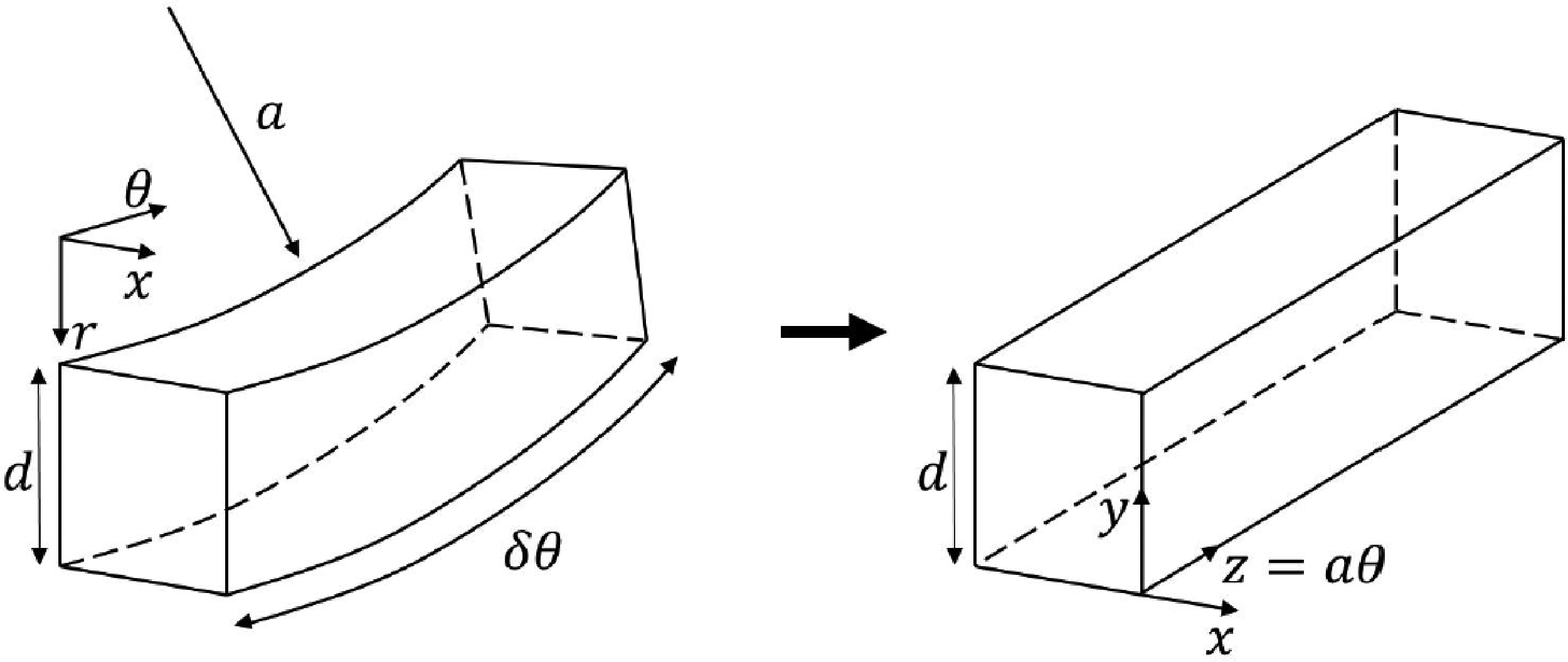
Approximation of the annular grooves into a rectangular section when $d\ll 1$ .

Annular groove model

The pressure field in the upper portion (region ②) of the annular groove can be expressed as a separable solution of the Helmholtz equation in cylindrical coordinates:

$$p(x,r,\theta )={\displaystyle \sum _{m=-\infty }^{\infty }{e}^{-jm\theta }}{\displaystyle \sum _{n=0}^{\infty }{f}_n}(x)g_{mn}(r)$$

(1)

where

$$f_n(x)=\cos ({\kappa }_{n}x),{\kappa }_n=\frac{n\pi }{l_g}$$

(2)

$$g_{mn}(r)=A_{mn}{J}_m({\alpha }_{n}r)+B_{mn}{Y}_m({\alpha }_{n}r)$$

(3)

and

$${\alpha }_n=\pm \sqrt{{\omega }^2-{\kappa }_n^2}$$

(4)

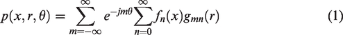
Here, A_mn and B_mn are arbitrary constants to be determined by boundary conditions at the septum. If it is assumed also that all higher-order modes are cut-off in the groove, which is true in the test geometry for all frequencies of interest (below 30 kHz), contributions to expression 1 for $n\ne 0$ can be neglected. Expression 1 then reduces to

$$p(x,r,\theta )={\displaystyle \sum _{m=-\infty }^{\infty }{e}^{-jm\theta }}\left[A_{m0}{J}_m(\omega r)+B_{m0}{Y}_m(\omega r)\right]$$

(5)

The boundary condition at the septum is:

$$\frac{{p|}_{r=1+d}}{{u_r|}_{r=1+d}}=Z_f$$

(6)

where Z_f is the locally reacting impedance of the septum and azimuthally partitioned cavity ①.

The radial particle velocity can be obtained by using the non-dimensional linearised momentum equation in the radial direction:

$$u_{r_n}(r)=\frac{j}{\omega }\frac{\partial p}{\partial r}=j\left[A_{m0}{J}_m\prime (\omega r)+B_{m0}{Y}_m\prime (\omega r)\right]$$

(7)

By substituting equations (5) and (7) into equation (6).

$$K_m=\frac{B_{m0}}{A_{m0}}=-\frac{J_m^{\prime }(\omega [1+d])+j\frac{J_m(\omega [1+d])}{Z_f}}{Y_m^{\prime }(\omega [1+d])+j\frac{Y_m(\omega [1+d])}{Z_f}}$$

(8)

Finally, the total effective impedance of a component of the acoustic field varying as $e^{-jm\theta }$ at the interface between the groove and the airway is given by

$$Z_g(\omega ,m)=\frac{{p|}_{r=1}}{{u_r|}_{r=1}}=-j\frac{J_m(\omega )+K_m{Y}_m(\omega )}{J_m^{\prime }(\omega )+K_m{Y}_m^{\prime }(\omega )}$$

(9)

The dependence of this quantity on ‘m’, the azimuthal mode number, demonstrates that this ‘impedance’ is not locally reacting in the sense that each azimuthal fourier component of the sound field in the airway experiences a different impedance. It also worth noting that for the case of a hard septum ( $Z_f\to \infty$ ), K_m is real and the impedance Z_g is purely reactive, as would be expected in the absence of any absorbing elements.

Cartesian groove model

An approximate expression can be obtained by assuming that the groove depth is sufficiently small ( $d\ll 1$ ) such that the annular casing can be approximated by a rectangular channel as indicated in Figure 3. The pressure field in the upper portion of the groove repeats itself over a distance $z=2\pi a(=2\pi )$ and may be written as a separable solution in Cartesian coordinates as

$$p(x,y,z)={\displaystyle \sum _{m=-\infty }^{\infty }{e}^{-j{k}_{z}z}}{\displaystyle \sum _{n=0}^{\infty }}\cos (k_{n}x)\left[A_{mn}\cos \left({\beta }_{mn}y\right)+B_{mn}\sin \left({\beta }_{mn}y\right)\right]$$

(10)

where

$$k_z=m,k_n=\frac{n\pi }{l_g}\text{ and }{\beta }_{mn}=\pm \sqrt{{\omega }^2-k_n^2-k_z^2}$$

(11)

Once again, only terms corresponding to n = 0 need to be considered giving

$$p(x,y,z)={\displaystyle \sum _{m=-\infty }^{\infty }{e}^{-\mathit{jmz}}}\left[A_{m0}\cos \left({\beta }_{m}y\right)+B_{m0}\sin \left({\beta }_{m}y\right)\right]$$

(12)

Following an analogous procedure to that for the annular groove, the expression for the effective impedance of the treatment (equation (13)) can be obtained by applying the boundary condition at the bottom of the groove (y = 0) and evaluating the pressure and particle velocity at the interface with the main duct (y = d). Note that the y-axis is defined in the opposite direction to the radius. This yields

$$Z_g(\omega ,m)=-\frac{j\omega }{{\beta }_m}\left[\frac{\cot ({\beta }_{m}d)+\frac{j\omega }{Z_f{\beta }_m}}{1-\frac{j\omega }{Z_f{\beta }_m}\cot ({\beta }_{m}d)}\right]$$

(13)

Once again, the configuration with hard septum can be modelled by setting $Z_f\to \infty$ in equation (13). As observed in expression 9, the acoustic impedance Z_g is not only a function of frequency but also of the azimuthal mode number m.

Comparison of groove models

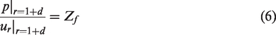
To assess the accuracy of the approximation of the annular grooves by a rectangular channel, Figure 4 shows a comparison of the impedance obtained with each model for a range of frequencies corresponding to the experimental data ( $0\le \omega \le 50$ ) and for the liner parameters shown in Table 1. In the case of the W-8 rig the duct radius is $\tilde{a}=279.4$ mm, giving a non-dimensional groove depth of 0.045. The impedance at the septum (Z_f) is obtained by using the standard non-dimensional expression for a SDOF cavity liner ⁸

$$Z_f=R_{fs}+j\left[\omega m_r-\cot (\omega h)\right]$$

(14)

where R_fs and m_r denote the non-dimensional resistance and mass reactance of the septum and $\cot (\omega h)$ is the reactance of the cavity.

Figure 4.

Comparison of the impedance models based on the annular (Model A) and Cartesian groove (Model B) for m = 22. (a) Hard septum. (b) Porous septum.

Table 1.

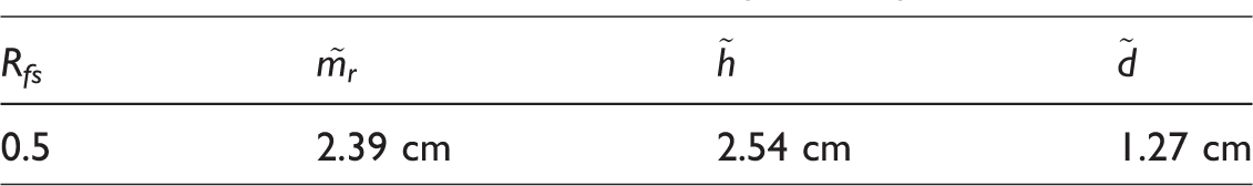
Numerical values used for the impedance parameters.

Rfs	$\widetilde{m_r}$	$\tilde{h}$	$\tilde{d}$
0.5	2.39 cm	2.54 cm	1.27 cm

Results are shown in Figure 4 for the cases of a hard and porous septum for m = 22. The agreement shown between the annular and Cartesian predictions is consistent with the results obtained at lower and higher azimuthal mode numbers. The two impedance models show good agreement for the whole range of frequencies used in this study. However, the annular model is used for the analytical predictions presented in the following sections.

Qualitative behaviour of the equivalent groove impedance

As indicated previously, the equivalent impedance for the case of a groove with a hard septum is obtained by setting 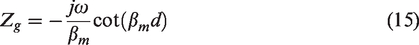$Z_f\to \infty$ in equation (13), yielding

$$Z_g=-\frac{j\omega }{{\beta }_m}\cot ({\beta }_{m}d)$$

(15)

The following implications about the groove behaviour can be immediately drawn

The liner presents a purely reactive response.

If $m=\omega ,Z_g=\pm j\infty$ (hard wall).

If m = 0, $Z_g=-j\cot (\omega d)$ (simple reactance behaviour).

If $m<\omega$ and $\omega =\sqrt{m^2+{\left(\frac{\pi }{2d}\right)}^2}$ , Z_g = 0 (pressure-release surface).

The behaviour with the porous septum is not as straightforward as in the hard septum case. The resistance, reactance and the normal incidence absorption coefficient of the groove with porous septum are shown in Figure 5 for a range of frequencies $0\le \omega \le 50$ , azimuthal mode numbers $0\le m\le 50$ and for the impedance parameters in Table 1. The normal incidence absorption coefficient of the impedance at the septum is also shown in Figure 5 as reference. The resistance of the lined groove, provided by septum, is no longer constant and depends on the frequency and azimuthal mode number. Both the resistance and the reactance show peaks around $m=\omega$ of a finite magnitude ( $Z_g\approx 20$ ) influenced by the impedance at the septum and the azimuthal propagation within the groove. However, the absorption coefficient of the groove is not substantially modified with respect to a SDOF cavity, the maximum attenuation in both cases occurs for Im(Z) = 0, that is at ω = 10 and ω = 38 in this example. The low-frequency limit shows that the impedance tends to $-\infty$ for the plane wave and to zero otherwise for both hard and porous septum.

Figure 5.

Groove impedance and normal incidence absorption coefficient for a range of frequencies $0\le \omega \le 50$ and azimuthal mode numbers $0\le m\le 50$ . (a) Resistance. (b) Reactance. (c) Absorption coefficient – groove. (d) Absorption coefficient – SDOF.

The radial propagation within the groove depends on the frequency and azimuthal mode number. The line $m=\omega$ separates two regions in the colormaps of Figure 5 that determine the propagation in the radial or y-direction that also apply to the hard grooves. If $m<\omega$ , k_y is real and waves are propagative in the radial direction (cut-on); if $m>\omega$ , k_y is imaginary and waves are exponentially decaying in the radial direction (cut-off).

High fidelity FEM simulations

A number of FEM computations have been conducted to assess the analytical models and their accuracy in predicting the equivalent impedance of the circumferential grooves both for hard and absorbing septums. The numerical simulations have been performed using the FEM commercial software Simcenter 3 D Acoustics. ⁷ A high-order FEM formulation is used within Simcenter, which uses adaptive polynomial order (p-refinement) in each element based on an a priori error indicator. The solver selects automatically the polynomial order in each element to obtain a target accuracy while minimizing the computational cost. This approach, described in Beriot et al., ⁹ is designed to tackle realistic large-scale 3 D problems over a large number of frequencies and only requires a single mesh.

The mesh creation process used in this instance follows the guidelines given in. ⁹ The mesh element size is selected as large as possible, constrained by the highest frequency of interest and the maximum polynomial order available. A target accuracy of 0.5% has been used. It should be noted that smaller elements are still required to ensure that the geometry at the boundaries is well represented and in regions where singularities are present.

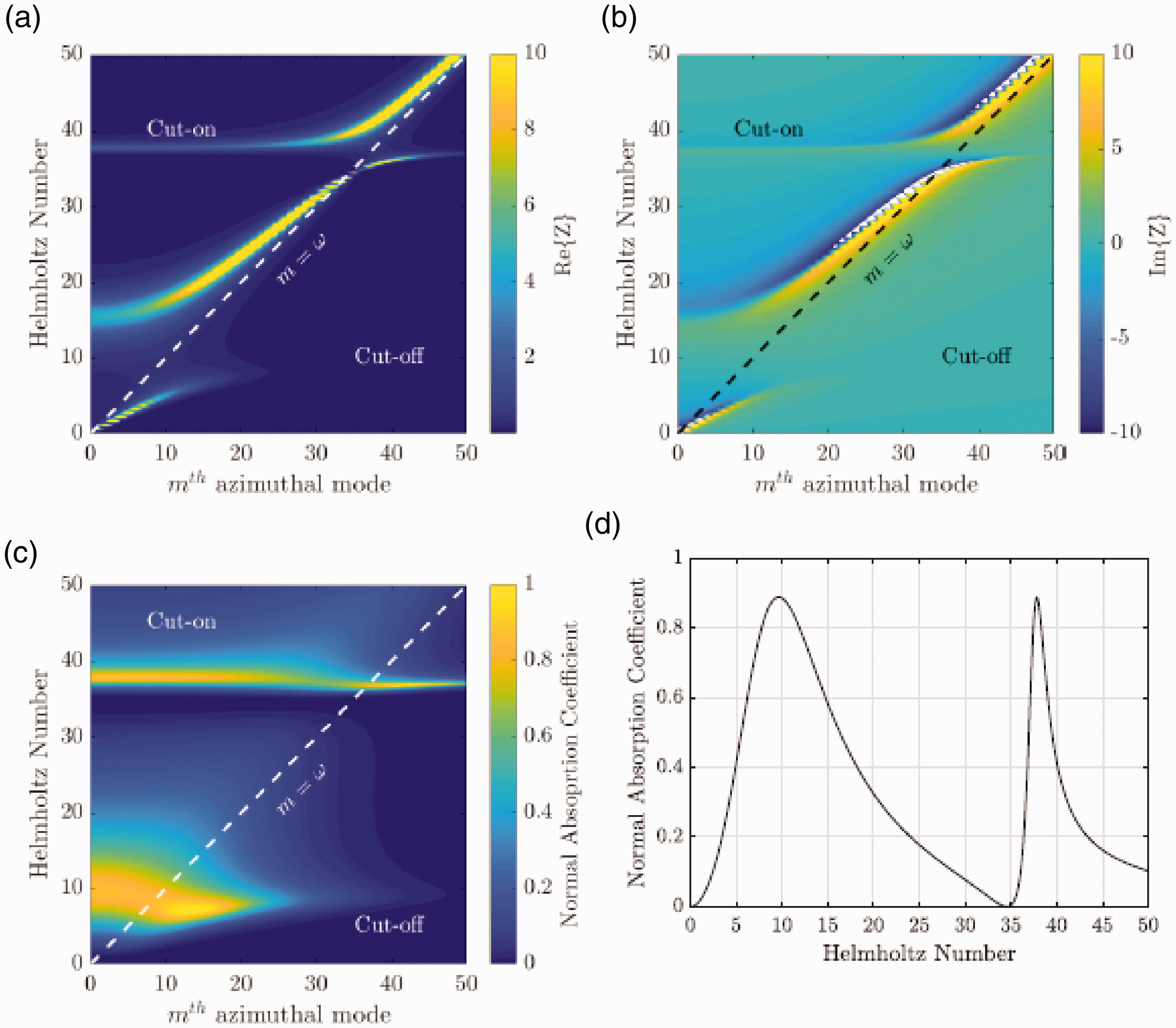
Three test cases have been performed, as shown in Figure 6:

Figure 6.

Diagrams of the FEM cases used for the verification of the analytical groove models. (a) Single groove with incident modes. (b) Multiple grooves with incident modes. (c) Application to OTR liners.

• Single groove with incident modes: the aim is to obtain the acoustic impedance within the open groove and at the interface with the main duct when excited by incoming duct modes of azimuthal and radial mode orders (m, n).

• Multiple grooves with incident modes: extension of the first case to six grooves, as used in the W-8 rig, to assess the variations on the impedance of each groove due to the interaction with adjacent grooves.

• Multiple grooves with a monopole source: consists of the full groove geometry and a monopole point source located at 95% of the radius. The aim is to assess the suitability of the analytic groove impedance model as an input wall impedance for OTR analytical prediction models described in. ⁴

All cases have been defined as 3 D finite ducts, numerically modelled by using a PML-type anechoic boundary condition at each end of the duct section. ⁷ The geometry of each circumferential groove is consistent with the dimensions of the grooves tested in the NASA W-8 fan rig. A hard septum and a SDOF locally reacting cavity impedance are imposed at the bottom of the open groove/s for the ‘hard’ and ‘lined’ groove configurations respectively.

A convergence study has been carried out for the single and multiple groove cases focusing on the refinement of the mesh close to the groove neck, of special interest to evaluate the equivalent impedance of the groove, and around the point source location. The cross-section of the mesh used for case (c) and a zoom around the groove region are shown in Figure 7.

Figure 7.

Cross-section of the mesh used for case (c) and a zoom around the groove region.

Verification of the analytical model with FEM results

Single groove with incident duct modes

In both of the analytical impedance models an assumption is made that the acoustic field is uniform across the width of the groove, i.e. that only the plane wave can propagate within the groove in the radial direction. However, it is expected that evanescent ‘cut-off’ components may contribute to the acoustic field at the open end of the groove where it matches to the external acoustic field in the airway. The standard deviation in acoustic pressure across the groove at a particular normalised depth, 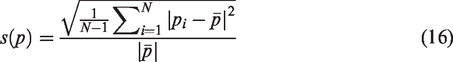$(r-a)/a$ , measured from the open end, is defined as

$$s(p)=\frac{\sqrt{\frac{1}{N-1}{\displaystyle {\sum }_{i=1}^N|}{p}_i-\overline{p}{|}^2}}{\left|\overline{p}\right|}$$

(16)

where N is the number of elements across the groove and the mean value ( $\overline{p}$ ) is given by

$$\overline{p}=\frac{1}{N}{\displaystyle \sum _{i=1}^N{p}_i}$$

(17)

The standard deviation across the groove of the pressure and radial particle velocity magnitudes in the FEM solution are shown in Figure 8 to assess the validity of the above assumption. The plots only show the results for the lined groove but the same behaviour has been observed for the hard groove. It can be observed that, as expected, the standard deviation is higher at the groove ‘neck’ (groove depth = 0), specially for the radial particle velocity: $s(p)\hspace{0.17em}\hspace{0.17em}\approx \hspace{0.17em}\hspace{0.17em}10\%$ and $s(u_r)\hspace{0.17em}\approx \hspace{0.17em}100\%$ , and is monotonically reduced when moving to the groove bottom (groove depth = 1): $s(p)(\%)\hspace{0.17em}\approx \hspace{0.17em}\mathcal{O}({10}^{-2})$ and $s(u_r)(\%)\hspace{0.17em}\approx \hspace{0.17em}\mathcal{O}({10}^{-2})$ .

Figure 8.

Axial standard deviation (in %) of the pressure and radial particle velocity within the lined groove for different incident modes (m = p1–18 (meaning 1 to 18, not exponential)) at 3900 Hz. Each colour represents a different azimuthal mode number and results are shown for the first three radial modes.

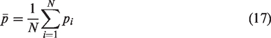
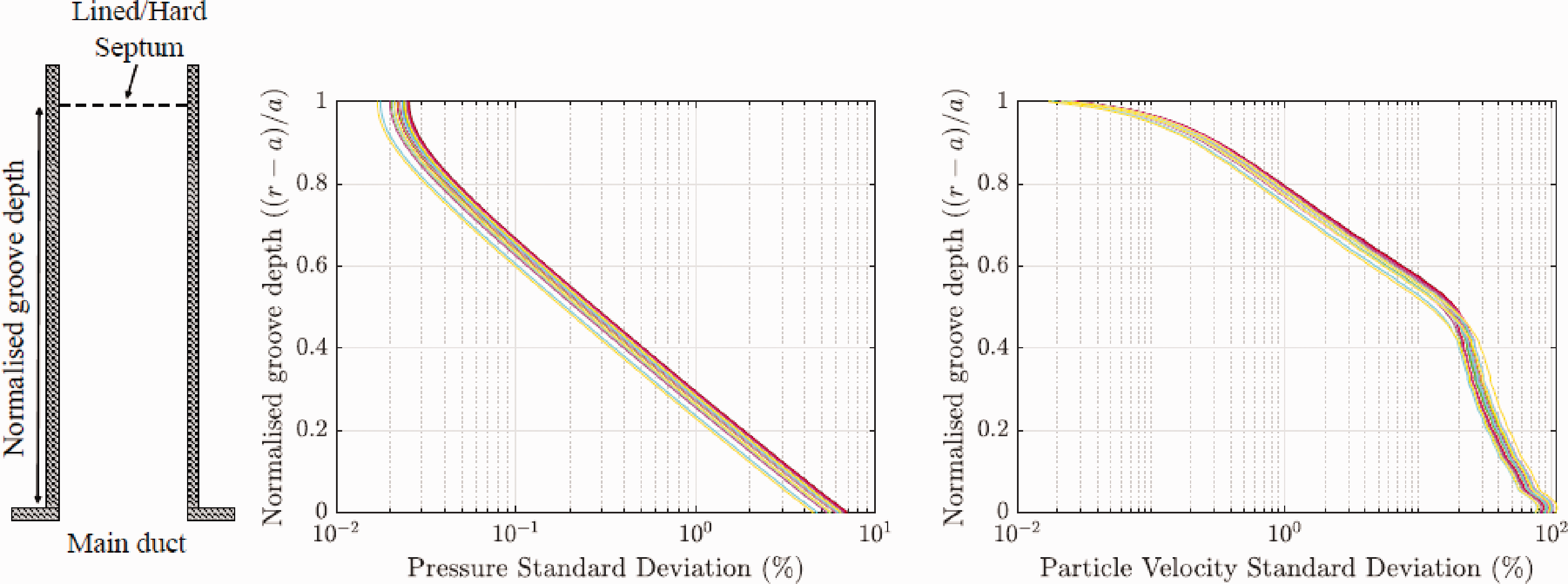
Results indicate that standard deviation in pressure and particle velocity is small across the duct and that an average value can therefore be compared to the analytical predictions. The equation of the groove effective impedance derived from the semi-locally reacting analytical model is based on a continuous solution of the wave equation throughout the groove and therefore the radial impedance at any point within the groove can be computed by evaluating the pressure and radial particle velocity at any radius, giving

$$Z_g(\omega ,m,r)=-j\frac{J_m(\omega r)+K_m{Y}_m(\omega r)}{J_m^{\prime }(\omega r)+K_m{Y}_m^{\prime }(\omega r)}$$

(18)

A comparison of the analytical and numerical effective impedance is shown in Figure 9 for a hard and lined duct, limited to modes (5,1), (15,1) and (20,1). In the hard groove case, the resistance is zero and the reactance results are in good agreement, tending to minus infinity when moving towards the hard wall boundary condition. In the lined groove case, both the resistance and the reactance satisfy the imposed boundary condition at the septum and generally present a satisfactory agreement.

Figure 9.

Radial impedance within the groove for different incident azimuthal modes: comparison of analytical annular model and numerical results at 3900 Hz. In the legend, A refers to Analytical and N to Numerical. (a) Hard groove. (b) Lined groove.

It is reassuring that the agreement between the analytical models and the FEM results is close within the groove. However, a good match of the equivalent impedance at the interface between the main duct and the groove, i.e. at normalised groove depth of zero, for the whole range of frequencies of interest and azimuthal mode numbers is also critical. This comparison is shown in Figure 10 for the lined groove and modes (5,1), (15,1) and (20,1). The numerical results are plotted for each mode only for the cut-on frequencies. A very good agreement can be observed, which has been shown to held for other azimuthal mode numbers and for the hard groove case.

Figure 10.

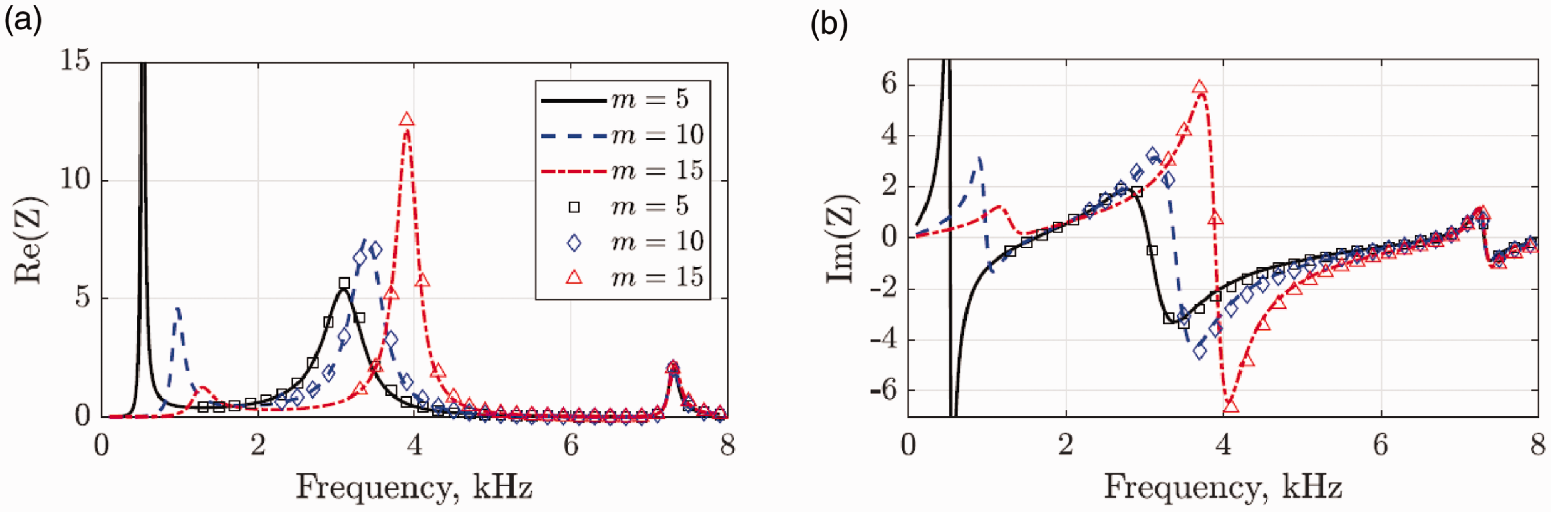
Frequency dependence of the effective groove impedance: comparison of analytical model and numerical results for the lined groove case. (a) Resistance. (b) Reactance.

These results indicate that the analytical groove models should provide an accurate prediction of the acoustic behaviour in the airway when applied as conventional impedance conditions in a uniform duct.

Multiple grooves with incident duct modes

The analytical impedance models are derived for a single groove but, in practice, multiple grooves are usually present, as in the fan casing tested in the W-8 rig. The extent to which the effective impedance of each groove is affected by the presence of adjacent grooves is now investigated using model (b) of Figure 6. Following a procedure analogous to that for the single groove, the numerical effective acoustic impedance $Z_{\text{num}}(\omega ,m,n,r)$ is evaluated at each of the six grooves considered in the geometry of Figure 6(b).

A comparison of the impedance predicted by the analytical single groove model with the numerical effective acoustic impedance obtained for the 6 grooves FEM model is shown Figure 11. Each of the six symbols per frequency correspond to values of the computed resistance/reactance for each groove at the open interface. It can be observed that the numerical impedance of each groove tends to cluster around the ‘single groove’ prediction with fairly small variations except at the peaks, where the impedance of the grooves is similar to that of a hard wall. In terms of relative error with respect to the single groove prediction, the results in Figure 11 range from 1% to 15%. This indicates that reasonable acoustic predictions can be expected if a multiple groove case is treated by assuming the effective impedance of a single groove applied to an extended duct length equivalent to that of the multiple groove liner.

Figure 11.

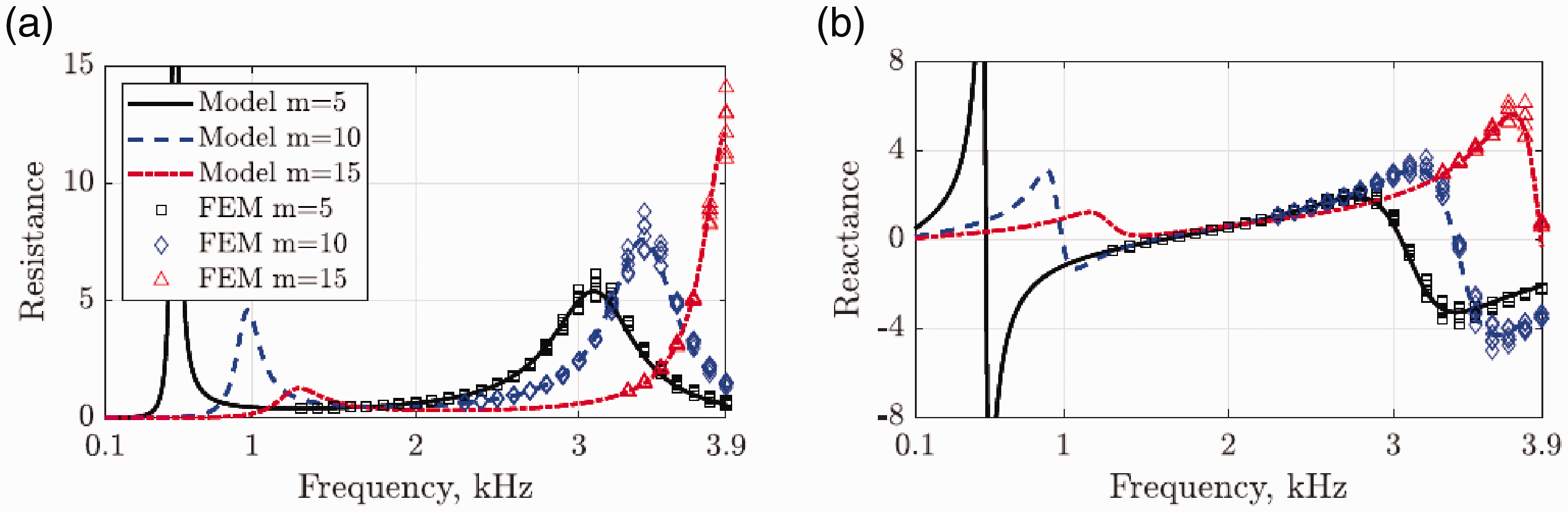
Frequency dependence of the effective groove impedance for multiple grooves: comparison of analytical model and numerical results for each groove for the lined groove case. (a) Resistance. (b) Reactance.

Application to OTR liners: multiple grooves excited by a point source

The ultimate aim of the groove impedance models is their application in predicting OTR liner fan noise suppression performance so that the analytical and numerical prediction models can be compared directly to the NASA W-8 rig experimental data. The description of the OTR analytical prediction model for propagation in the fan duct and a preliminary comparison with the experimental data is covered in. ⁴ The model relies on a Green function approach for a point source close to the liner surface. In this section a preliminary attempt is made to assess the use of the impedance prediction from the groove model as input for the OTR analytical prediction model. It also quantifies the effect on axial sound power attenuation of applying the single groove impedance when multiple grooves are present in the geometry.

The OTR analytical model, called Green/FINF, consists of a cylindrical finite lined section connected to infinite hard wall duct extensions. The acoustic field is excited by a monopole or dipole point source located close to the lined surface. This is a simplification of a more realistic configuration where an OTR liner (modelled by the lined section) is used to suppress fan sources (modelled with equivalent point sources above the liner). Monopole-type and dipole-type sources are commonly used for modelling aerodynamic fan noise: monopoles represent the volume displacement caused by the aerofoil thickness and dipoles the force exerted by the fan blades on the fluid. ¹⁰ The problem is shown in Figure 12. The acoustic field is obtained in Green/FINF by imposing continuity of mass and momentum at the two interfaces: I-II and II-III and has been cross-verified for a constant impedance in the lined section against FEM simulations for zero and uniform mean flow. The numerical FEM model in this case is that of Figure 6(c) which represents the full geometrical character of the six grooves and their hard or lined septums.

Figure 12.

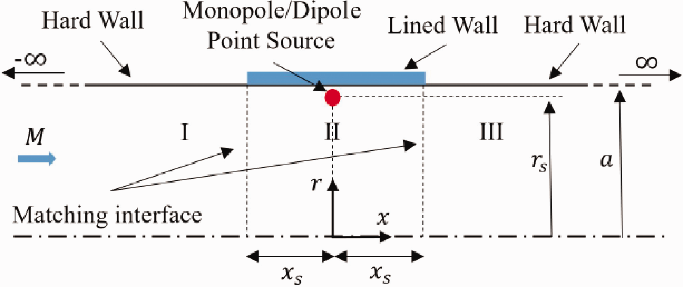
Diagram of the OTR analytical prediction model.

The lined circumferential grooves are defined in the Green/FINF model by a corrected impedance obtained from the analytical groove models and the length of the treatment ( $2x_s$ ). Two alternatives have been explored and compared to the FEM results. These are:

Use the impedance of a single groove and a shortened liner length equal to the groove open area or groove-duct interface. This approach does not account for the effect of the hard walls between grooves. i.e. define

$$Z_{\text{eff}}=Z_g,2x_s=6l_g$$

(19)

Use a corrected impedance based on the continuity of mass in the radial direction to account for the rigid surfaces between the groove cavities. i.e. define the length of the liner as the total length of the acoustic treatment and use a porosity correction $\sigma =l_t/l_g$ , which in this case is $\sigma =3/2$ . i.e. define

$$Z_{\text{eff}}=\sigma Z_g,2x_s=l_t=6(l_g+l_s)$$

(20)

The non-dimensional acoustic axial power at each axial cross-section (S) is computed by integrating the intensity field over the duct cross-section, resulting in^11–13:

$$P(x)={\displaystyle {\int }_S{I}_x}dS=\frac{1}{2}{\displaystyle {\int }_{S}R}e\left\{p{u}_x^{*}\left(1+M^2\right)+Mp{p}^{*}+M{u}_x{u}_x^{*}\right\}\mathrm{d}S$$

(21)

where p, u_x and M are acoustic pressure, the acoustic particle velocity in the axial direction and the Mach number respectively.

The PWL Insertion Loss quantifies the reduction in acoustic power due to the liner by subtracting the power level obtained in the presence of the liner ( $P_{\text{lined}}$ ) from that obtained in a baseline hard wall case ( $P_{\text{hard}}$ ):

$$\text{PWL IL}(x)=10{\text{log}}_{10}\frac{P_{\text{hard}}(x)}{P_{\text{lined}}(x)}[dB]$$

(22)

The PWL IL obtained with the analytical prediction model and the two alternatives described above are compared to the FEM results in Figure 13. Although both alternatives generally show a good agreement, the use of a corrected impedance applied to the total length of the acoustic treatment (alternative (b)) shows a better agreement, especially in the region of higher attenuation (1–2.5 kHz). The differences between the analytical prediction (b) and the FEM solution are less than 0.2 dB for the whole frequency range. The alternative without the porosity correction over-predicts the attenuation of the acoustic treatment by up to 1 dB relative to the FEM solution. This result was expected by the authors since the porosity assumption is a better representation of the physical problem and has been widely used in liner modelling. ⁸

Figure 13.

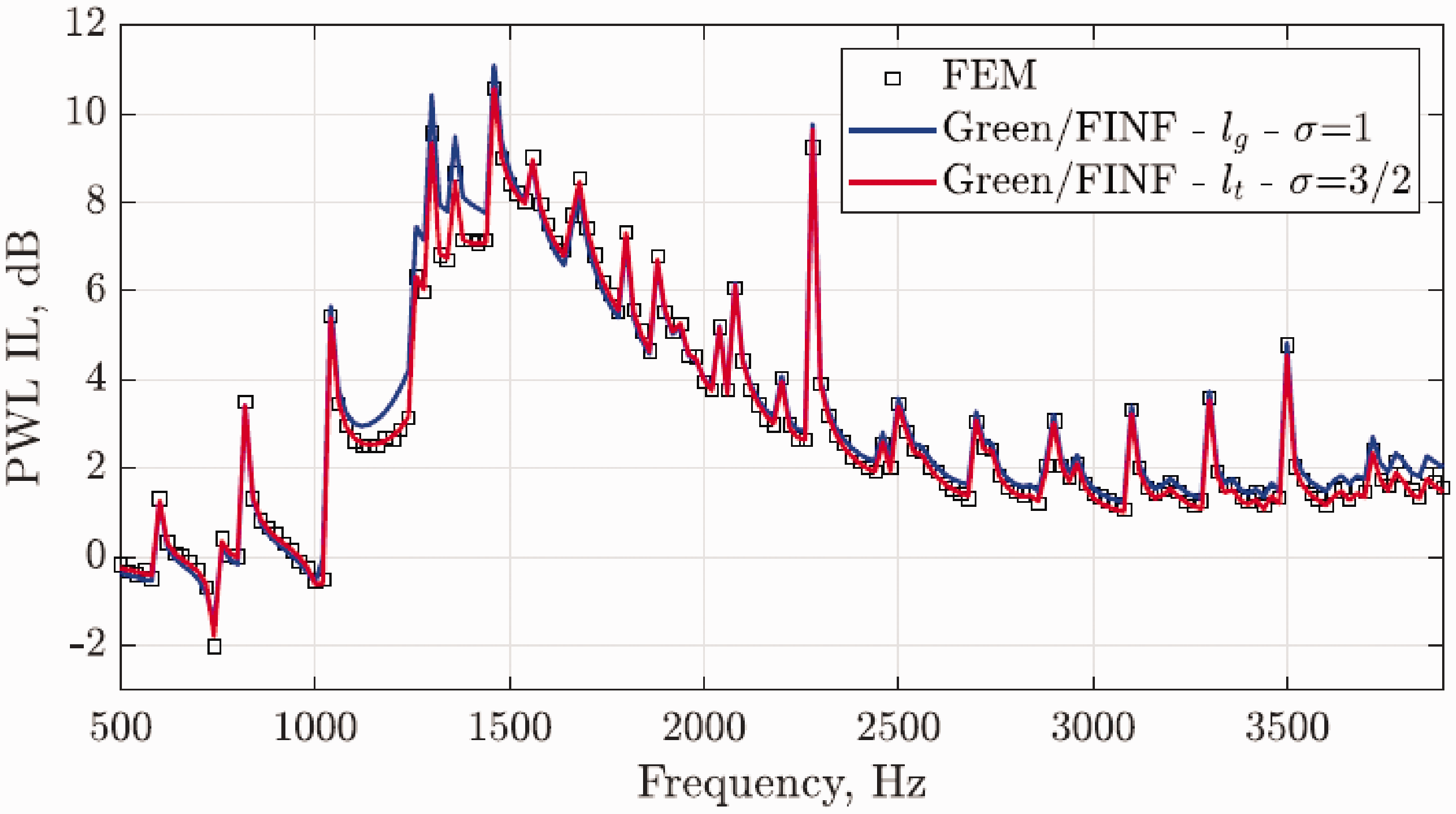
Comparison of PWL Insertion Loss analytical predictions against the FEM results for a monopole point source.

A key factor of having grazing flow over the grooves is the excitation of cavity resonances. Additional groove or cavity noise in the presence of the OTR grooves treatment was measured at certain frequency ranges in the tests conducted in the W-8 rig. ³ Testing of the same OTR casing treatments in the NASA Grazing Flow Impedance Tube showed the generation of cavity noise at the same frequency range than when installed over a turbofan rotor. ¹⁴ The lengthwise tones caused by the feedback loop of the unstable shear layer over the cavity ¹⁵ cannot be predicted in the analytical groove impedance model nor the FEM solver due to the inviscid nature of the Helmholtz equation and it is out of the scope of this work.

Conclusions

The work reported here has been undertaken within a broader project to improve the understanding of OTR liner acoustic performance by using analytical models based on monopole and dipole Green's functions for lined cylindrical ducts. The validation of analytical predictions against experimental data from a recent OTR circumferential groove array tested in the NASA W-8 fan rig, requires an analytical model for the impedance of the OTR configurations used in the experiments.

The OTR treatments modelled consist of circumferential grooves extending over an axial length equal to the axial projection of the fan chord. The grooves are formed of upper and lower parts. The upper part is open at the top and terminated at the base with a hard or porous ‘septum’. Below the septum the lower part of the groove is partitioned azimuthally. Two analytical models have been developed, one exact and the other approximate; the former assumes that the groove area of the treatment is annular as in the experiment; the approximate model assumes that the groove depth is small in comparison to the radius, which can then be ‘unwrapped’ and treated as a rectilinear channel. These are termed annular and Cartesian models. Both are ‘semi-locally reacting’ in the sense that local reaction is assumed in the axial direction, but non-local reaction in the azimuthal direction. That is to say, the impedance depends on the frequency and the azimuthal mode number. Good agreement between the two impedance models has been established for the geometry and frequencies of interest in this project.

The locally/non-locally reacting behaviour assumed in the development of the analytical models have agreed with the FEM high-order, high-fidelity numerical simulations for the range of frequencies of interest, which consist of a 3 D axisymmetric duct with a single groove and incident duct modes. Good agreement has been found between the predicted analytical groove impedance and the numerical impedance evaluated in the groove-duct interface of the FEM model.

An extension of the FEM model to include multiple grooves has indicated also that the effective impedance of each groove tends to cluster around the ‘single groove’ prediction with fairly small variations except at peak values, where the behaviour of the grooves is practically that of a hard wall. This suggests that the use of the analytical single groove impedance model in cases with multiples grooves can provide reasonable predictions.

The groove model has been applied to OTR liners by using it as an input for a simplified OTR analytical prediction model, Green/FINF. The test case consists of a cylindrical finite lined duct section matched to infinite hard wall duct extensions excited by a monopole point source located within the lined section. The analytical predictions for PWL insertion loss obtained by using the direct ‘single groove’ impedance and with a corrected effective impedance based on a porosity factor have been compared to the FEM predictions accounting for the full groove geometry. The use of the porosity-corrected impedance has been found to be more accurate than the use of the actual impedance over a shorter liner length. Differences relative to the FEM solution did not exceed 0.2 dB for the whole frequency range. The predictions based on the direct ‘single groove’ impedance has been found to differ by up to 1 dB from the FEM solution.

Additional cavity noise due to grazing flow over the cavities cannot be modelled with the analytical impedance models and is outside the scope of this work. Future work in groove modelling might also include consider effects of the swirling flow within the groove induced by the rotation of the fan blades. This would require swirling flow to be present also in the main duct and to be consistent with that in the groove.