Sage Journals: Discover world-class research

Abstract

Ducted propellers are an interesting design choice for unmanned aerial vehicle (UAV) concepts due to a potential increase of the propeller efficiency. In such designs, it is commonly assumed that introducing the duct also results in an overall noise reduction. The objective of this work is to experimentally analyze and quantify noise of a ducted propeller suitable to be installed on a medium size UAV (wingspan 5–10 m). A microphone array is used for recording the noise levels at each microphone position and used collectively to localize noise sources with beamforming. Different types of noise sources are considered (an omni-directional source and a propeller). In addition, the effect of the presence of an incoming airflow is assessed. With no incoming airflow, it is found that the duct significantly modifies the noise radiation both in the frequency and the spatial domain. With an incoming airflow, the effect of the duct on the frequency content of the signal is almost eliminated. The fact that for this case the harmonics become lower results in a reduction of the received noise levels. Also the directivity changes. These insights are of importance in efforts towards modeling the effects of ducts for complex noise sources such as propellers.

Keywords

Ducted propeller beamforming UAV noise reduction thrust correction microphone array

Introduction

The flexibility and wide range of possible applications make unmanned aerial vehicles (UAVs) an object of continuous research. An important focus of such work is the propulsion system and ways of improving its efficiency. UAVs operate at low Reynolds numbers, meaning that the viscous effects are predominant, which decreases the efficiency of the propellers.^1,2 A ducted propeller is a common solution to increase the efficiency of the propulsion system,^3,4 which is especially beneficial for UAVs driven by electric motors due to their limited battery capacity.⁵ The duct increases the mass flow rate by reducing the slipstream contraction, increasing the overall thrust, and suppressing vortex shedding. This suppression leads to a reduction in tip induced drag.^6,7 Additionally, ducts provide protection by containing the blades in the event of blade failure.

A ducted propeller is thus commonly referred to as a way of improving the propulsive efficiency of the UAV but also as a way of reducing noise emissions,^8,9 although recent work indicates a slight increment of noise when a hard wall duct, without lining, is introduced.¹⁰

Sound propagation in a duct poses a complex problem. The total sound pressure field is expected to consist of a superposition of different propagating modes in the axial and the radial direction of the duct (azimuthal and radial modes).¹¹ Higher frequency content of sound sources generates more modes, and per mode, the sound is expected to cut off at a certain frequency and decay exponentially in the lengthwise direction of the duct. This theoretical behavior is well understood for an infinite duct with and without axial flow. Work has been done to obtain approximations for semi-infinite ducts.¹² Still, prediction of sound propagation in finite ducts poses to be a difficult task and is usually estimated computationally. This becomes even more cumbersome in case a complex source such as a propeller is considered.

For propellers, the noise consists both of tonal and broadband noise.^9,13 The different mechanisms that originate broadband noise are for example, the blade tip clearance, and the interaction of the wake generated by the fan blades with the duct boundary layer.

This work aims to experimentally assess the effect of a hard wall duct on the noise radiation of a propeller. Dimensions of the duct and the propeller used in the experiments are typical of a medium size UAV with a wingspan of 5–10 m.¹⁴ The noise measurements are performed in an open-jet anechoic wind tunnel facility, with and without incoming airflow.

The design of the duct is out of scope of this work and the main objective is the characterization of the noise radiation of a simple duct, which serves as a baseline for later modifications.

An acoustic array is used to determine the noise levels at different microphone positions, providing a wide range of observer positions relative to the source. The microphones are used individually to record the levels of sound and collectively to perform beamforming. Beamforming identifies the most important sound sources in the experiments and as such is an indispensable tool to understand the noise radiation.

As a first step, the noise behavior of an omni-directional source in the duct without incoming flow is considered. In this way, the resultant noise radiation is only due to the mode propagation and reflections inside the duct, and diffraction by the edges. The omni-directional source is then replaced by the propeller and the two cases are compared. The propeller has a strong noise directivity and the wake generated by the blades interacts with the duct, which affects noise radiation. As a next step, experiments are conducted with the ducted propeller under a uniform incoming airflow and the results are compared with the measured levels in case no flow is present.

When the duct is introduced, the propeller thrust changes, which affects the noise characteristics of the propeller. Therefore, changes in noise radiation verified between the ducted and unducted propeller can erroneously be attributed to the duct alone when in fact they are also due to changes of propeller noise. A final experiment investigates this effect by adjusting the rotational speed in order to obtain the same thrust for the isolated and ducted propeller. This clarifies how much the duct alone influences noise radiation.

Up to the authors’ knowledge, this is the first time the combined effect of a duct on both thrust and noise radiation is investigated. This work also contributes to a clearer assessment of noise attenuation by a duct and as such contributes to future designs of ducts and measures such as lining for reducing the acoustic footprint of an UAV.

The “Signal processing” section presents the methods used for assessing individual microphone pressure levels and beamforming. The section “Experiment” discusses the experimental setup, describing the duct and propeller geometry as well as the acoustic room and the microphone array. The “Results” section presents the findings of the different experiments. The final section presents the conclusions of this work.

Signal processing

In this work, the sound is recorded using a microphone array. A common way of presenting a change in the noise level due to a shielding object is based on the factor ΔL_p in dB, given by a ratio of the root-mean-square (RMS) signals

Δ L_{p} = 20 \log_{10} (\frac{p_{rms}^{object}}{p_{rms}^{source}})

(1)

The term ΔL_p is commonly referred to as shielding factor. In the experiment, this factor is obtained from the case where the propagation of sound from the source to the receiver is obstructed by the duct, $p_{rms}^{object}$ , and when there is no obstruction, $p_{rms}^{source}$ . Negative values indicate a decrease of the sound level resulting from the placement of the duct.

The power spectral density (PSD) is determined for the individual microphones, and the average is taken over the microphones to obtain the averaged PSD. For the spectra shown throughout this work, the PSD is integrated over consecutive (narrow) frequency bands. In this work, a band of 5 Hz is chosen. The spectrum level relative to p₀ = 20 µPa is then obtained as

L_{p} (f_{band}) = 10 \log_{10} (\frac{\int_{band} S (f) d f}{p_{0}^{2}})

(2)

for the PSD given by S(f) for frequency f. L_p (f_band) is the sound pressure level in dB for f_band.

The overall sound pressure level (OSPL) of the signal is determined as

L_{p} = 10 \log_{10} (\frac{p_{rms}^{2}}{p_{0}^{2}})

(3)

where p_rms is determined over the time signal. Equation (2) reduces to equation (3) if the band encompasses the whole frequency range of the signal.

Using the microphones of the acoustic array allows to evaluate the sound pressure levels (SPLs) for various observer locations, positioned at different directions from the source. Additionally, it is possible to use the microphones collectively to obtain the position of the sources and their SPLs. This is known as beamforming. Beamforming is a widely applied signal processing technique to spatially filter the signals to either directionally receive or transmit a signal. To perform beamforming, a time delay is applied to each microphone depending on the spatial position of interest. Summation of the delayed signals for all microphones provides the beamformer output for the given position. The method of conventional beamforming used in this work is explained in detail in the Appendix 1.

In this work, beamforming is used to visualize the source distribution, i.e., diffraction from the duct leading and trailing edges, for the different experiments. Beamforming also helps investigating the differences of the isolated propeller with and without incoming airflow and it is useful to identify external sources generated in the experimental setup that can affect the results.

Experiment

Duct geometry and noise sources

The duct used in the experiment is custom built at the TU Delft and is based on a Clark-Y profile. Although this is not a very efficient profile, it was selected so the propeller has constant tip clearance from x/c = 0.3 m, which is useful for other experiments. This duct is not a final design, but simply a baseline for future modifications.

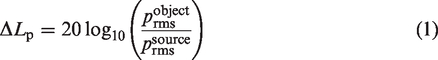
A cut section of the aluminum duct can be seen in Figure 1. The inner diameter of the duct is 30 cm, the chord length is 15 cm and the thickness is 11.7% of the chord length.

Figure 1.

Cut section of the duct. The airfoil is a Clark-Y profile with chord of 15 cm. The inner diameter of the duct is 30 cm. The dotted cross at the center of the duct indicates the position of the omni-directional noise source and propeller.

Two different noise sources were used in the experiments: an omni-directional source and a propeller. Both sources are centered in the duct in the radial and axial direction as seen in Figures 1 and 2. The distance of the source relative to the array is fixed at 1.46 m.

Figure 2.

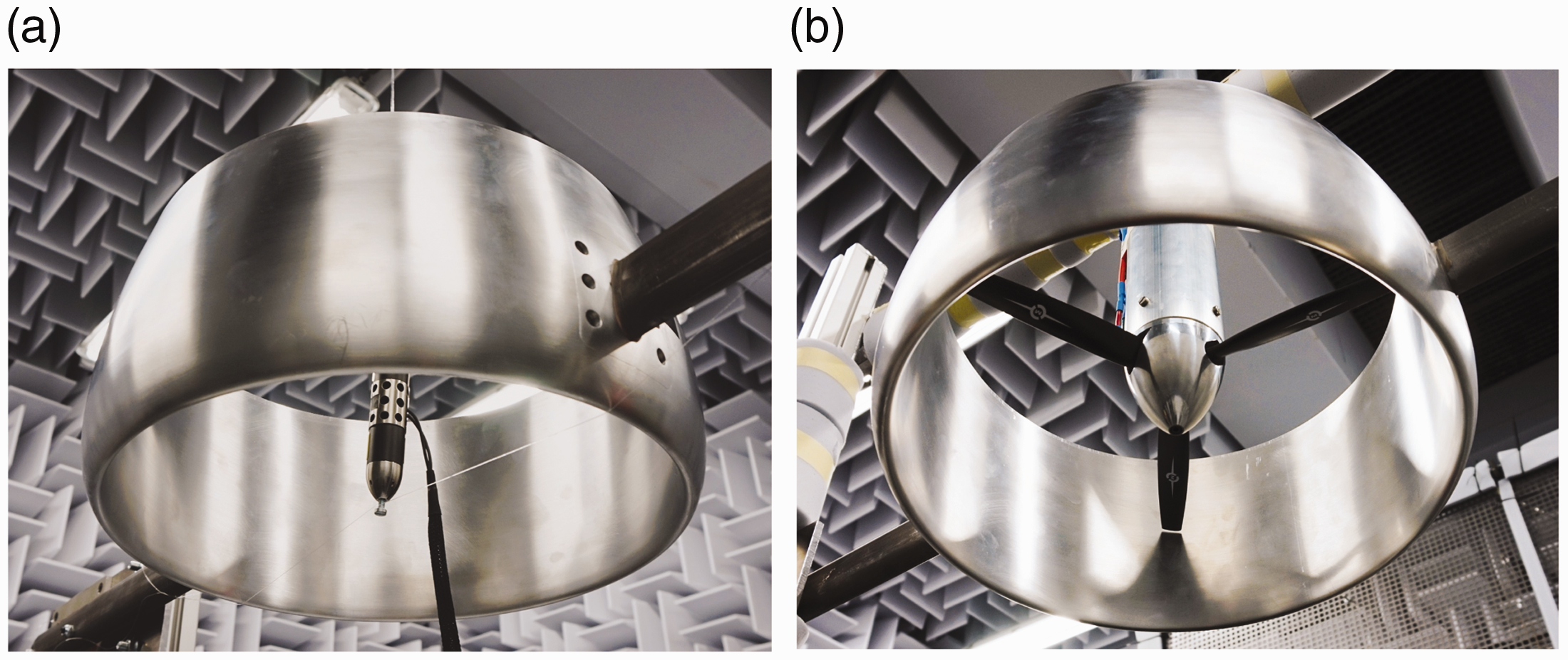
The omni-directional source and the propeller positioned in the center of the duct. (a) The omni-directional source. (b) The propeller.

The omni-directional source is a customized Miniature Sound Source type QindW developed by Qsources™. It has an oblong shape with a length of 11 cm and a diameter of 2.0 cm. The sound source has a flat frequency response from approximately 0.50 to 6.3 kHz when driven by white noise.

The small three-blade propeller is a Master Airscrew E-MA1260T and is connected to a Kontronik PYRO 700–45 Brushless motor. The motor is controlled with an electronic speed control using a Kontronik Jive PRO 80+ HV. The diameter of the propeller was initially 30 cm, but it was trimmed in order to have a tip clearance of 2 mm inside the duct. The propeller was 3D scanned (Figure 3) to obtain an approximate geometry and airfoil for the simulations (see Appendix 2).

Figure 3.

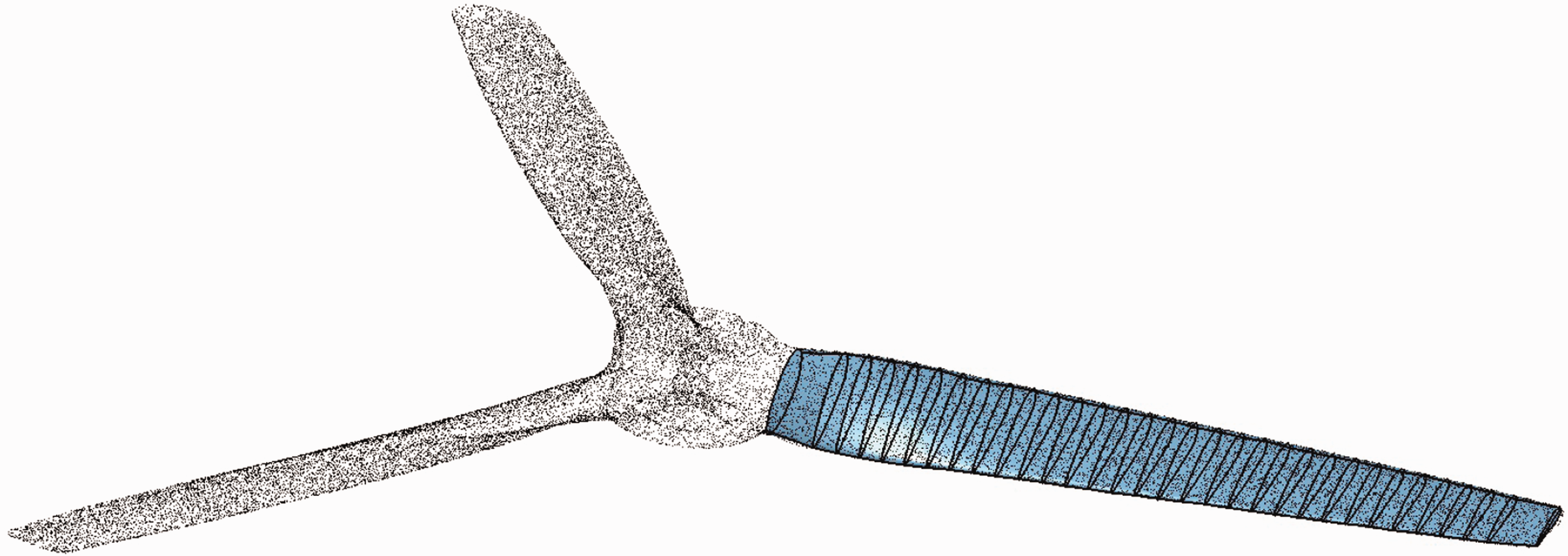
3D scan of the propeller (black dots) and blade reconstruction in CATIA™.

In the experiments with the propeller, the power applied to the motor terminals was varied between 35% and 90% of the maximum power (210 W). In the results presented, the propeller was set at 85%, corresponding to a rotational speed of 7500 r/min. Other values of rotational speed were also analyzed but led to the same conclusions.

Anechoic room and microphone array configuration

The noise is measured using a microphone array consisting of 64 G.R.A.S. 40PH CCP free-field array microphones¹⁵ The microphones were calibrated individually using a G.R.A.S. 42AA pistonphone.¹⁶ The data acquisition system is composed of 5 National Instruments PXIe-4499 sound and vibration data acquisition modules controlled by a NI PXIe-8370 remote control module and a NI RMC-8354 controller. The uncertainty associated to the measurements of the acoustic array was experimentally determined as 0.5 dB.

The structure of the array was designed to reduce acoustic reflections while allowing different microphone array configurations.¹⁷ The free-field behavior of the anechoic room was assessed following the guidelines of the ISO3745.¹⁸ All frequency bands above 315 Hz fulfill the standards.¹⁹ The average reverberation time is 0.25 s, which corresponds to the anechoic category of ISO3382.²⁰ The background noise was assessed and it is such that it is not expected to interfere with the noise measurements.¹⁹

The test section is placed in the center of the anechoic room (5.4 m by 5.4 m) and has a circular shape with a 60 cm diameter. This means that the ducted propeller is contained in the jet. The experimental setup is illustrated in Figure 4.

Figure 4.

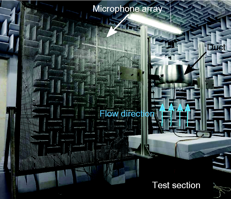
The experimental setup in the Anechoic Vertical Low Turbulence Wind Tunnel at the TU Delft. The duct is positioned in front of the TU Delft optimized array consisting of 64 microphones with an aperture of 1.9 m.

The microphone configuration used is the TU Delft Optimized Array distribution,^21,22 which provides the best trade-off between the Main Lobe Width and Maximum Side lobe Level in beamforming. The recording time for every microphone is set to 60 s.

Results

Comparison of noise from ducted and unducted sources

Omni-directional source

The first case analyzed is the omni-directional source with no incoming airflow. There is no disturbance of the medium and the noise is affected only by the mode propagations of the duct, reflections, and subsequent diffraction by the leading and trailing edge.

The PSD is obtained as an average over the microphones and is shown in Figure 5. The red line corresponds to the source only and is, as expected, approximately flat over frequencies of 400–6000 Hz. With the duct present, the spectrum changes, showing a periodic behavior, as expected for sound propagation in ducts. In general, there will be resonance and anti-resonance frequencies inside the duct.^23,24 Furthermore, it is expected that different propagation modes will be generated each having its own cut-off frequency.^25,26 As the duct used in this experiment is an open duct of small length, the exact behavior in the far field is hard to predict. Still, typical duct behavior can be seen in Figure 5. As the omni-directional sound source is relatively flat in the given frequency range, Figure 5 can also be seen as an approximated frequency response of the duct observed at the position of the array. To investigate whether a change in directivity also occurs due to the duct, Figure 6 shows the noise changes in terms of OSPL at the microphone locations.

Figure 5.

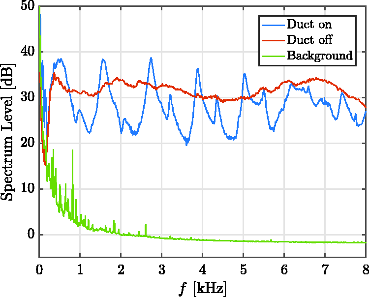
Averaged spectrum level over the microphones in the array for the omni-directional source in red and the modified spectrum with the duct on in blue. The green line indicates the background spectrum with the source off.

Figure 6.

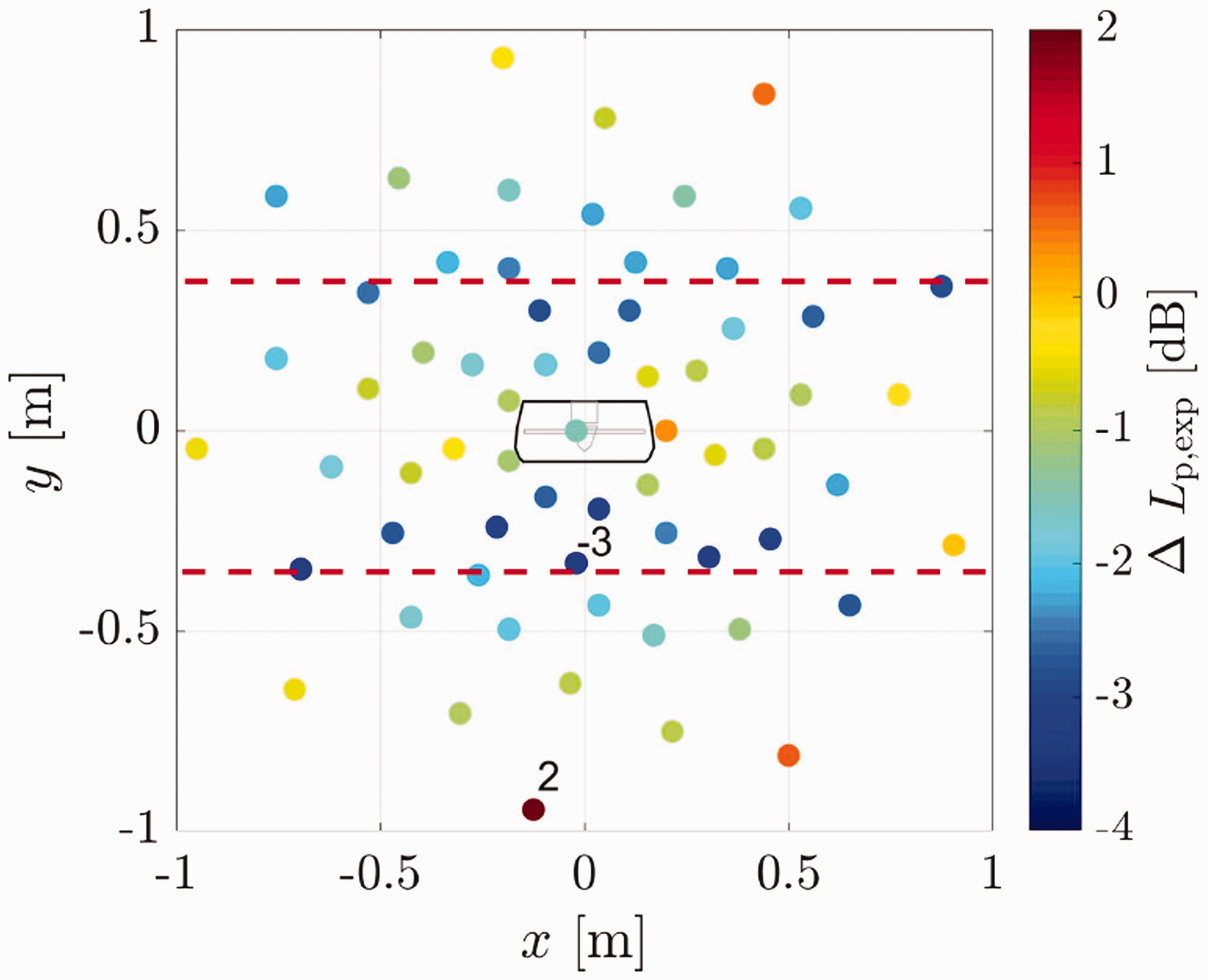
Difference in OSPL of the omni-directional source over the acoustic array (bandpass filtered between 400 Hz and 6000 Hz) when the duct is introduced. The outline of the duct on the array is shown in the center. The red dashed lines at y = ±0.35 m indicate the region with maximum values of noise reduction.

Negative values indicate noise reduction when the duct is introduced (values calculated using equation (1)) and positive values indicate amplification of noise. Two bands can be distinguished from the figure for which there is a reduction of roughly 2 to 3 dB at y = ±0.35 m (red dashed lines). At y = 0 m, which is at the center of the duct, there appears to be a slight reduction of the noise level of around 1 dB, a value that is close to the uncertainty associated to the measurement (0.5 dB). This region is in the shadow zone, which implies that the resulting sound is mostly due to diffraction by the duct’s edges. There is some constructive interference for locations at the top and bottom of the microphone array with reinforcement of noise around 2 dB.

It can be concluded that placing the duct significantly affects the measured PSD but effects with regards to directionality are limited (3 dB).

Propeller without incoming airflow

The PSD of the propeller set at 85% of the maximum power, with no incoming airflow, is shown in Figure 7, both without duct (in red) and with duct (in blue). The spectrum of the ducted omni-directional source (in gray) is shown for comparison purposes. It is clear that there is an increase of noise for most frequencies when the duct is introduced, except for the first harmonic. Compared to the isolated propeller, the harmonics are no longer visible for frequencies above 2 kHz. Whereas the ducted propeller shows a PSD with a smooth oscillating behavior that is similar to that of the ducted omni-directional source, the frequencies of resonance and anti-resonance have changed completely.

Figure 7.

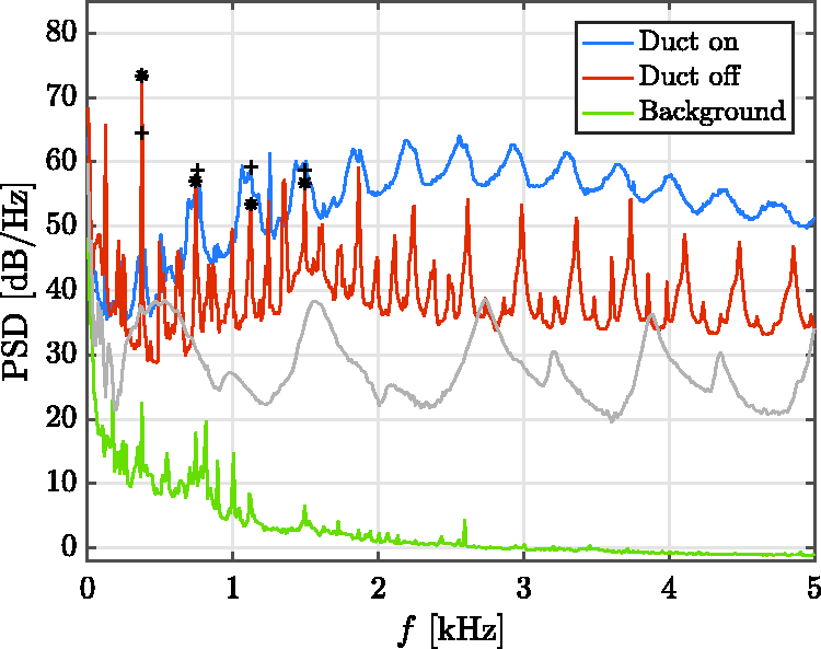
Averaged spectrum level over the microphones for the propeller at 85% of the maximum power corresponding to a propeller speed of 7500 r/min. The stars and crosses indicate the BPF and its first three multiples for the isolated and ducted propeller, respectively. As a comparison the ducted omni-directional sound source is shown in gray.

A clear change in directivity is visible from Figure 8, showing the difference in OSPL with and without the duct. No regions with reduced levels of noise are present and an increase of noise up to 12 dB is found at the top and bottom of the array. The spatial behavior is very different from that observed for the omni-directional source. The lower increase in noise level is at the center of the array, in contrast to what was observed in Figure 6.

Figure 8.

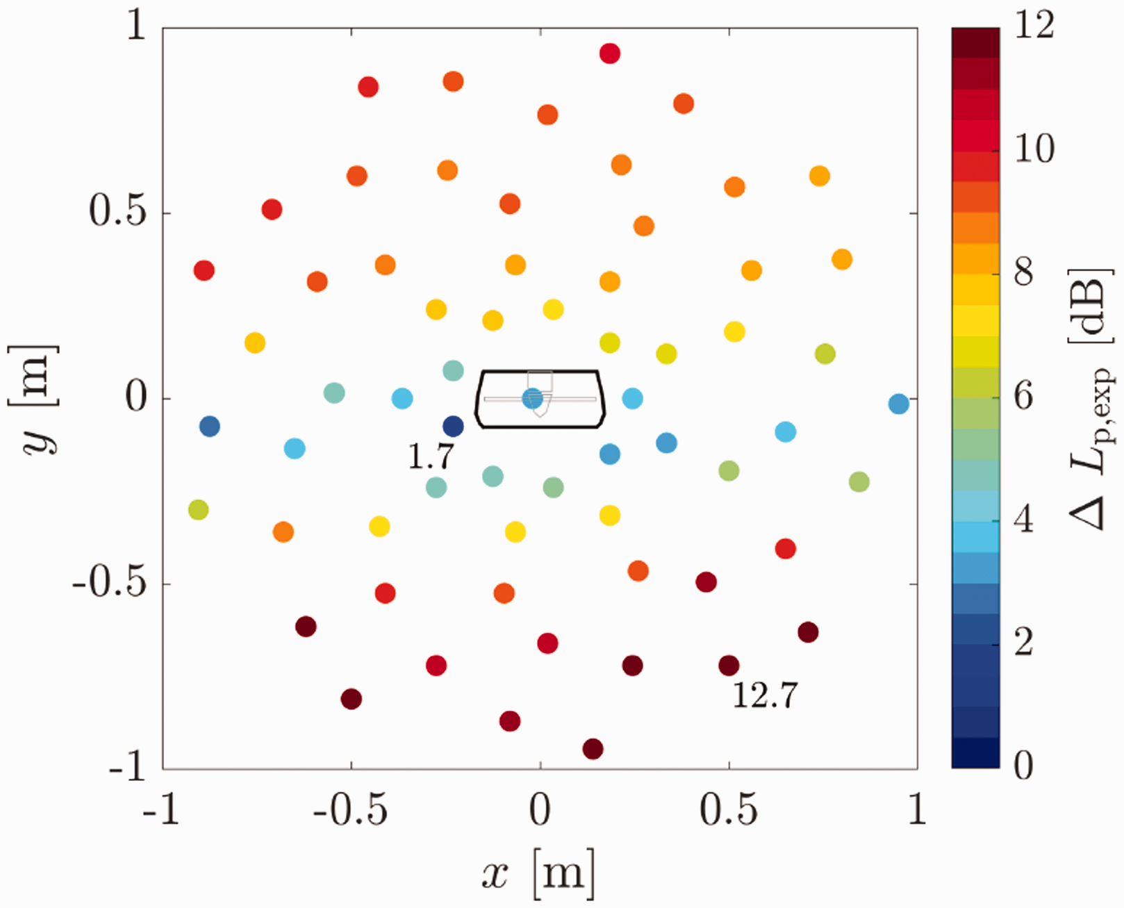
Difference in OSPL for the propeller at 7500 r/min, with no incoming airflow, in the acoustic array when the duct is introduced (filtered between 50 and 8000 Hz). The outline of the duct on the array is shown in the center.

It can be concluded that again, the PSD is completely modified due to the placement of the duct. In contrast to the omni-directional source, now only increases in noise levels are found. This is hypothesized to be due to the creation of additional broadband noise sources as the propeller disturbs the quiescent medium and creates for example, trailing edge noise due to the propeller slipstream interaction with the duct. In addition, the directivity significantly changes due to the placement of the duct (see Figure 8). This means that when considering noise of a ducted propeller its radiation properties, both in the frequency and spacial domain, cannot be directly derived from the isolated propeller properties.

Propeller with incoming airflow

Figures 9 and 10 show the effect of placing the duct around the propeller in case of airflow (10 m/s), on the PSD and the spatial distribution of the noise levels. The placement of the duct results in a slight increase of broadband noise, but a decrease in the levels of the harmonics. The latter is reflected in Figure 10, showing significant reduction in noise levels for all microphones. Compared with the situation without airflow, still the lower levels of noise are located at the center of the array.

Figure 9.

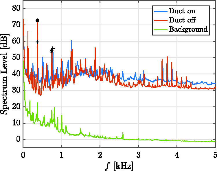
Averaged spectrum level over the microphones in the array for the propeller set at 85% of the maximum power (with airflow at 10 m/s), and the modified signal with the duct on. The stars and crosses indicate the BPF and its first multiple for the isolated and ducted propeller, respectively.

Figure 10.

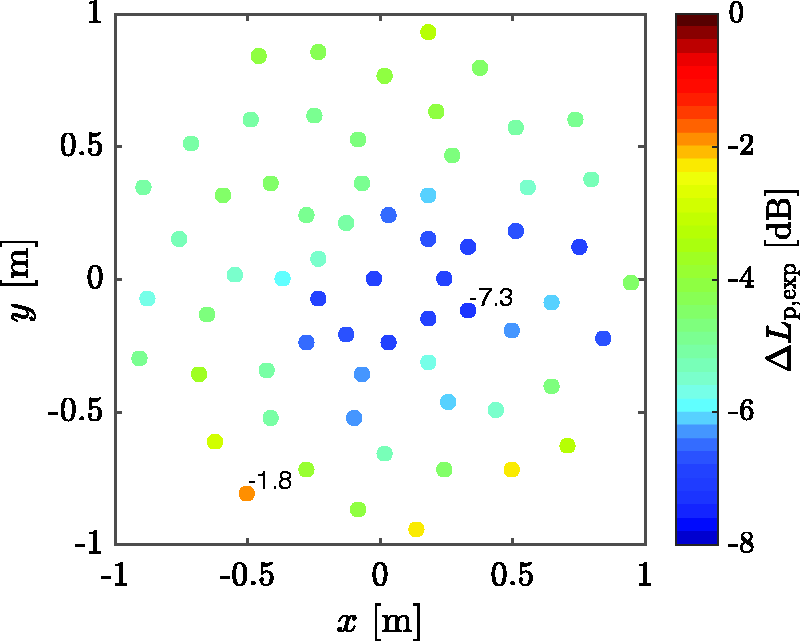
Difference in OSPL of the propeller at 7500 r/min, with incoming airflow, in the acoustic array when the duct is introduced (filtered between 50 and 8000 Hz). The outline of the duct on the array is shown in the center.

The effect of the duct now is very different compared to the case without airflow. Apparently the duct placed around a propeller with no incoming airflow creates an additional noise source, represented by the blue line of Figure 7. We hypothesize that this noise originates from the tip vortices interaction with the duct walls. These sources remain up their location as there is no airflow upstream. An observation supporting this hypothesis can be the relatively close agreement between the blue and gray line of Figure 7, representing a typical duct propagation. The absence of this source (blue line in Figure 8) in the case with airflow no longer dominates (and thus reveals) the PSD of the isolated propeller. These assumptions will be further investigated in the next section where beamforming is applied to localize noise sources.

Beamforming

As a first step the ducted omni-directional source is considered, as this reflects a typical duct propagation configuration. Peaks and valleys of Figure 5 were chosen for beamforming between 2 and 6 kHz, i.e., multiple frequency bands were chosen for either the valleys or peaks in this range. The frequency of 2 kHz was chosen as it is higher than the Rayleigh criterion so that sources at both sides of the duct can be discerned. The upper frequency of 6 kHz was chosen as it is close to the upper frequency limit for which the source could reliably emit sound omni-directional. In the case of noise reduction (Figure 11(a)), the main source is located on the leading edge. However, for the case which corresponds to amplification of noise (Figure 11(b)), there are sources of equal magnitude on the leading and trailing edges of the duct, reflecting variations in duct propagation with frequency.

Figure 11.

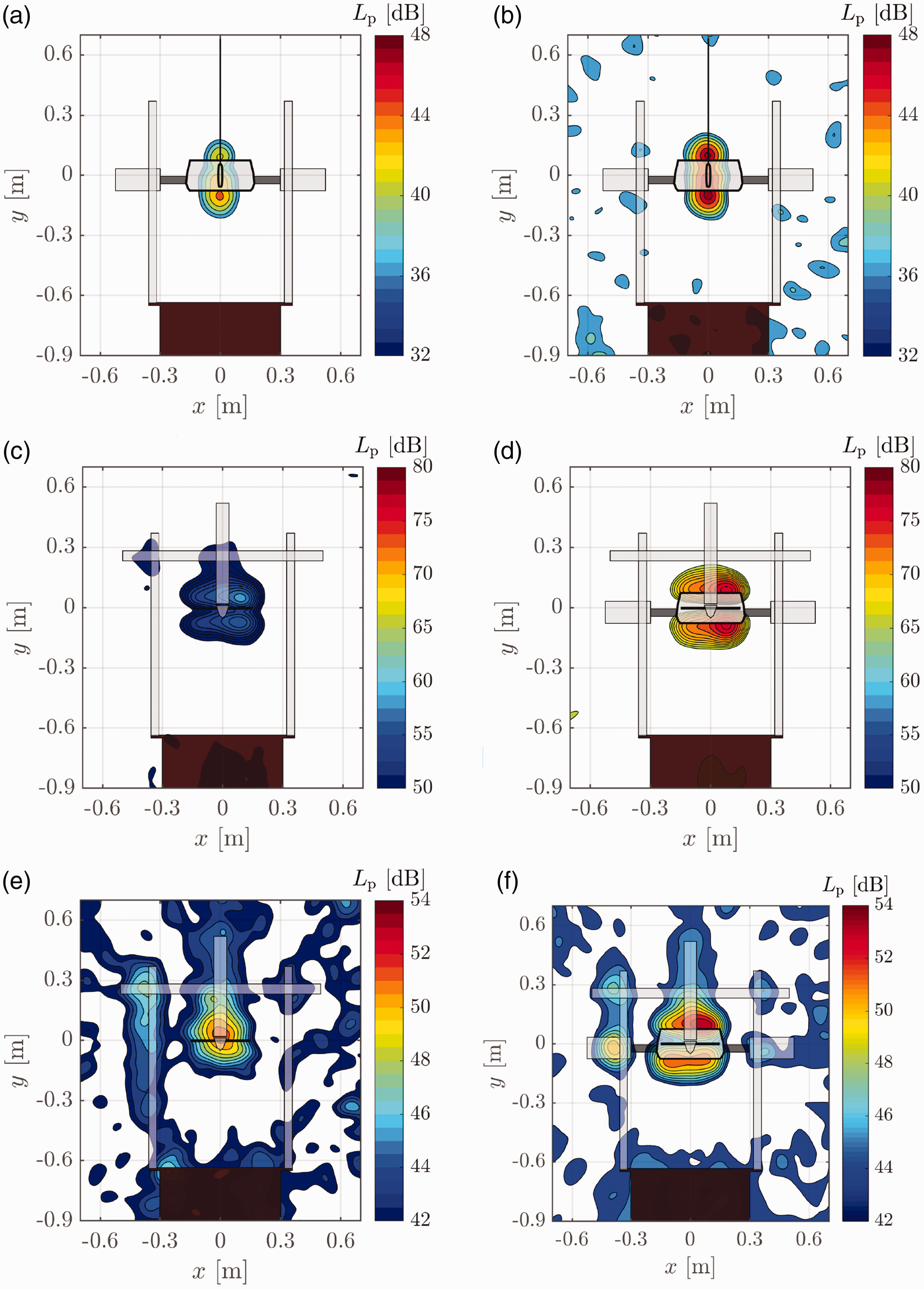
Beamforming of the omni-directional source for frequencies of the peaks and valleys observed in Figure 5, and for the isolated and ducted propeller with and without incoming inflow. (a) Valleys. (b) Peaks. (c) Isolated propeller, with no incoming airflow. (d) Ducted propeller, with no incoming airflow. (e) Isolated propeller, with a constant incoming airflow. (f) Ducted propeller, with a constant incoming airflow.

In the case of the propeller, noise decrease is observed mostly at the first harmonic (according to the spectra of Figure 8) but beamforming of such a low frequency does not provide enough resolution to clearly identify noise sources. Therefore, beamforming was performed between 2 and 5 kHz.

It appears that the propeller noise sources without the duct do not lie exactly on the propeller plane as seen in Figure 11(c). The main source for both figures is located at the right which is the direction of the propeller rotation towards the array. Similar behavior was seen in previous work,²⁷ where beamforming would not exactly position the sources at the propeller plane for certain tones due to the source being non-compact and coherent. Under no airflow, the beamforming plots of the isolated and ducted propeller (Figure 11(c) and (d)) are very different. Not only the strength of the noise sources increases as the duct is introduced, but also a new noise source is identified at the leading edge. This confirms the hypothesis stated before that the combined effect of the resonance (as also observed for the omni-directional source) and the interaction of the turbulent flow with the duct are the reasons behind an increase of noise levels.

The beamforming plots with incoming airflow of Figure 11(e) and (f) reinforce such assumptions since in this case there is no evidence of new noise sources when the duct is introduced. The slight increase of broadband noise between 2000 and 5000 Hz is the responsible for the 2 dB increase between Figure 11(e) and (f). The constant airflow moves the turbulent noise sources upstream resulting in diffraction effects on the edges but not so much in duct propagation. No localized noise sources are seen on either of the duct edges.

Noise of a ducted propeller with thrust corrections

In the previous section, the same power was used for the isolated propeller and ducted propeller, and the maximum value of noise reduction found was around 7 dB (Figure 10). However, the duct affects the performance of the propeller, which results in a different value of thrust¹⁰ for the same power of the motor. In this section, it is evaluated if correcting the power, in order to obtain the same value of thrust for the isolated and ducted propeller, affects significantly the noise levels.

In this subsection, it is experimentally determined for which rotational speed of the propeller the value of thrust is the same with and without the duct. Subsequently, the effect of the duct on noise radiation is reevaluated. The method used to determine the thrust experimentally which is briefly explained below.

The thrust coefficient is approximated from

C_{T} = \frac{2 π}{16 ρ n_{rev}^{2} R^{4}} \int_{0}^{R} Δ p_{s} d r_{p}

(4)

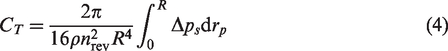
Here ρ is the air density, R is the radius of the propeller, n_rev is the number of rotations per second, r_p the distance to the root of the propeller, and Δp_s is the difference in static pressure before and after the propeller disk plane.

In this work, the static pressure p_s is approximated using the value of the total pressure p_t, since only small differences are expected between the total and static pressure in this experiment, conducted under low-speed conditions.

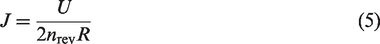
The advance ratio of the propeller, J, was varied between 0.26 and 0.42, and the incoming flow was set constant at 10 m/s. The advance ratio is calculated using

J = \frac{U}{2 n_{rev} R}

(5)

with U the undisturbed flow speed.

The thrust is determined for each value of J, both for the isolated and ducted propeller. Therefore, once all the values of J and C_T are determined, it is possible to determine which values of J correspond to the same C_T for the ducted and isolated propeller. This is done by the means of linear interpolation.

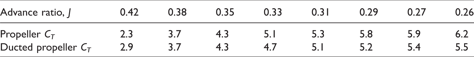
The value of Δp_t (≈Δp_s) is determined by measuring the total pressure upstream of the propeller and in the free stream, using two Pitot tubes. The Pitot tube in the free stream is fixed and the Pitot tube upstream of the propreller disk is moved from the root to the tip of the blade in increments of 1 cm. This experimental setup is shown in Figure 12 and the thrust coefficients obtained for the isolated and ducted propeller are displayed in the first and second row of Table 1, respectively.

Figure 12.

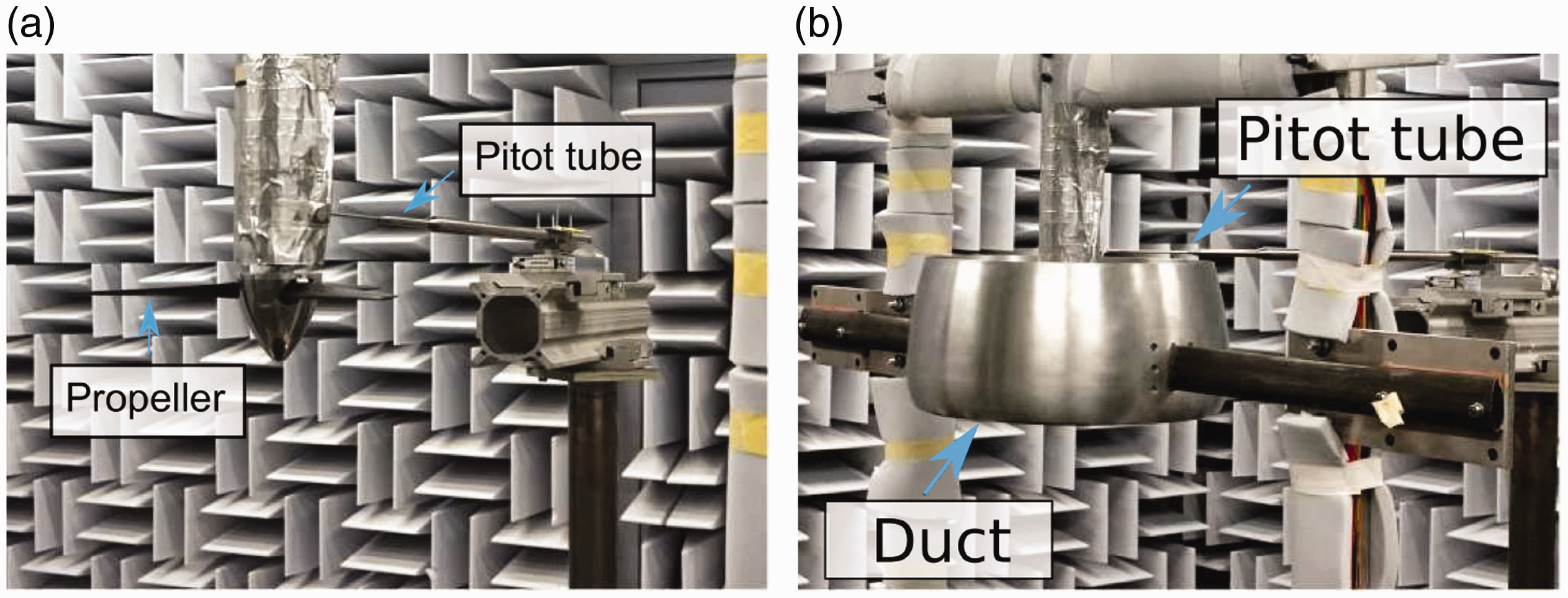
Setup used in the experiment to measure the thrust of the propeller. (a) Isolated propeller. (b) Ducted propeller.

Table 1.

Values of thrust coefficients C_T (×10²) with and without the duct and with a constant incoming flow for advance ratios J.

Advance ratio, J	0.42	0.38	0.35	0.33	0.31	0.29	0.27	0.26
Propeller C_T	2.3	3.7	4.3	5.1	5.3	5.8	5.9	6.2
Ducted propeller C_T	2.9	3.7	4.3	4.7	5.1	5.2	5.4	5.5

In Appendix 2, a model is used for predicting C_T to confirm that indeed the measured C_T values are of the order of magnitude as theoretically expected.

The experimental results of Table 1 are used to find the advance ratio J for which the propeller and the ducted propeller have the same value of C_T. Table 2 shows the results for two selected values of C_T. For the lower values of J, the thrust coefficient is higher for the isolated propeller than for the ducted propeller, indicating that the geometry of the duct is not the best design choice from a performance perspective.

Table 2.

Interpolated values of advance ratio (J) for equal values of the thrust coefficient.

Configuration	Advance ratio, J	C_T × 10^–2
Isolated Propeller	0.310	5.3
Ducted propeller	0.302
Isolated Propeller	0.270	5.9
Ducted propeller	0.263

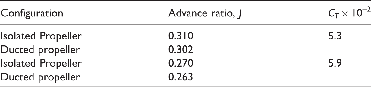
The values of C_T were selected based on typical operational conditions during flight (corresponding to 75% and 85% of the total power). The corresponding propeller settings (J) do not differ much when corrected for the same thrust (less than 5% of relative difference) but still can affect noise levels. Therefore, the ducted propeller was set at the new values of J of Table 2 and the noise levels were measured again at the microphone array.

Figure 13 shows the histogram of the measured noise reduction by placing the duct when the rotational speed of the propeller is kept constant (red line) and when it is adjusted for the same thrust (black line). For the first case interpolated in Table 2, represented in Figure 13(a), the majority of the microphones show noise reductions of –2 dB for both the adjusted and non-adjusted rotational speed. So, no significant error is obtained in this case by not considering the same thrust for the isolated and ducted propeller. However, for the second value of C_T, the histograms of Figure 13(b) are different. Before considering the same thrust for the isolated and ducted propeller the majority of the microphones correspond to noise reduction values of around –6 dB, and after the correction, this value is around –2 dB.

Figure 13.

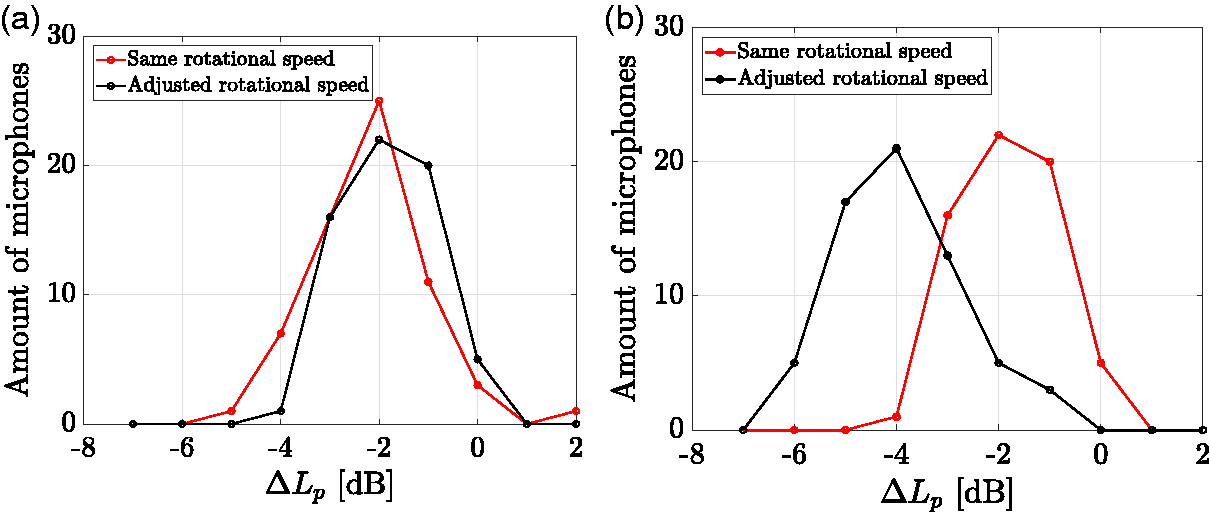
Histogram of ΔL_p: Propeller and ducted propeller generating thrust equal to (a) C_T = 5.3 × 10⁻² and (b) C_T = 5.9 × 10⁻².

Therefore, the values of noise reduction due to placing a duct as presented in the previous section with airflow (seen in Figure 10) were overestimated. This leads to the conclusion that the noise reduction for the same propeller rotational speed is also a consequence of the reduction of thrust caused by placing the propeller inside the duct and not only of the duct acting as a barrier between the noise source and observers.

Conclusions

The rapid increase of the UAV applications has initiated the need for capabilities to model the noise radiated by these systems. Typical UAV propulsion systems consist of a ducted propeller and as such a model for the noise radiation of these ducted propellers is needed. In this contribution, as a step towards the development of these models, experiments have been conducted to investigate the characteristics of noise radiation from ducted propellers.

From experiments with an omni-directial noise source and a propeller, without incoming airflow, it is found that using measurements for the unducted case will not provide relevant information for the case with a duct placed around the noise source. The noise radiation behavior, once the duct is placed, changes drastically. Either complex modeling or dedicated measurements are needed to predict the noise radiation for the ducted case.

In case airflow is present the situation changes completely, and now the noise radiation from the unducted and ducted case are highly similar. It is hypothesized that in this case the turbulent structures created by the propeller are convected with the airflow and that as such these moving sources do not result in a source configuration that induces duct propagation.

The effects of the duct on the PSD are limited to:

Increasing broadband noise,

Decrease of the first harmonics.

For the case considered, an overall decrease in noise level was found. But as stated above, the PSD of the unducted case is representative for the ducted case.

As such, this work has shown that using source characteristics measured without a duct can be used for modeling purposes in case a duct is introduced, since always airflow will be present in real applications. This especially holds for the PSD but can also be an initial assumption for the directivity.

For assessing the effect of the duct on the overall sound level, it is important to ensure that the aerodynamic performance of the propeller does not change due to the presence of the duct. An experimental investigation concluded that significant deviations can be present if this effect is not taken into account.

Footnotes

Declaration of conflicting interests

The author(s) declared no potential conflicts of interest with respect to the research, authorship, and/or publication of this article.

Funding

The author(s) received no financial support for the research, authorship, and/or publication of this article.

Appendix 1—Beamforming Method

References

MacNeill

Verstraete

Blade element momentum theory extended to model low Reynolds number propeller performance. Aeronaut J 2017; 121. DOI: 10.1017/aer.2017.32.

Oliveira

Muñoz

Catalano

Aerodynamic analysis of high rotation and low Reynolds number propeller. In 48th AIAA/ASME/SAE/ASEE joint propulsion conference & exhibit. Atlanta, GA: American Institute of Aeronautics and Astronautics.

Yilmaz

Erdem

Kavsaoglu

Performance of a ducted propeller designed for UAV applications at zero angle of attack flight: an experimental study. Aerospace Sci Technol 2015; 45: 376–386.

Martin

Tung

Performance and flowfield measurements on a 10-inch ducted rotor VTOL UAV. Technical report, Army Research Development and Engineering Command Moffett Field CA Aviation Aeroflight Dynamics Directorate, 2004.

Gur

Rosen

Optimizing electric propulsion systems for unmanned aerial vehicles. J Aircraft 2009; 46: 1340–1353.

Akturk

Camci

Influence of tip clearance and inlet flow distortion on ducted fan performance in VTOL UAVs. AHS Forum 2010; 338: 111–121.

Yilmaz

Erdem

Kavsaoglu

Effects of duct shape on a ducted propeller performance. In 51st AIAA aerospace sciences meeting including the new horizons forum and aerospace exposition, Grapevine (Dallas/Ft. Worth Region), Texas, AIAA Paper 2013-0803. DOI: 10.2514/6.2013-803

Moore

MD.

NASA personal air transportation technologies. Technical report, SAE Technical Paper, 2006.

Oleson

Patrick

Small aircraft propeller noise with ducted propeller. In 4th AIAA/CEAS aeroacoustics conference. p. 2284.

10.

Pereira

JL.

Hover and wind-tunnel testing of shrouded rotors for improved micro air vehicle design. College Park: University of Maryland, 2008.

11.

Devenport

Glegg

Aeroacoustics of low Mach number flows: fundamentals, analysis, and measurement. Cambridge: Academic Press, 2017.

12.

Gabard

Astley

Theoretical model for sound radiation from annular jet pipes: far-and near-field solutions. J Fluid Mech 2006; 549: 315–341.

13.

Marte

Kurtz

DW.

A review of aerodynamic noise from propellers, rotors, and lift fans. Pasadena, CA: Jet Propulsion Laboratory, California Institute of Technology, 1970.

14.

Fahlstrom

P and

Gleason

Introduction to UAV systems. Hoboken, NJ: John Wiley & Sons, 2012.

15.

G.R.A.S. Sound & Vibration - 40 PH CCP Free-field array microphone, https://www.gras.dk/products/special-microphone/array-microphones/product/178-40ph (accessed 14 January 2010).

16.

G.R.A.S. Sound & Vibration – 42AA Pistonphone class 1, https://www.gras.dk/products/calibration-equipment/reference-calibrator/product/255-42aa (accessed 14 January 2010).

17.

Vlemmix

Acoustic array design: the design of a reconfigurable phased microphone array for aeroacoustic wind tunnel measurements. 2017.

18.

ISO norm 3745 – acoustics – determination of sound power levels and sound energy levels of noise sources using sound pressure – precision methods for anechoic rooms and hemi-anechoic rooms. Technical report 3 (International Organization for Standardization, 2012).

19.

Merino-Martinez

Microphone arrays for imaging of aerospace noise sources. 2018.

20.

ISO norm 33382 – acoustics – measurements of room acoustics parameters. Technical report 1 (International Organization for Standardization, 2012).

21.

Malgoezar

AMN

Snellen

Sijtsma

, et al. Improving beamforming by optimization of acoustic array microphone positions. In 6th Berlin beamforming conference. BeBeC-2016-S5.

22.

Luesutthiviboon

Malgoezar

AMN

Snellen

, et al. Maximizing source discrimination performance by using an optimized array and adaptive high-resolution clean-SC beamforming. In Berlin Beamforming Conference 2018.

23.

Ingard

Singhal

VK.

Effect of flow on the acoustic resonances of an open-ended duct. J Acoust Soc Am 1975; 58: 788–793.

24.

Curtis

Nelson

Elliott

, et al. Active suppression of acoustic resonance. J Acous Soc Am 1987; 81: 624–631.

25.

Kinsler

Frey

Coppens

, et al. Fundamentals of acoustics. 4th ed. pp. 560. Weinheim: Wiley-VCH, 1999.

26.

Rienstra

SW.

Fundamentals of duct acoustics. Von Karman Institute Lecture Notes 2015.

27.

Horvath

Envia

Podboy

GG.

Limitations of phased array beamforming in open rotor noise source imaging. AIAA J 2004; 52: 1810–1817.

28.

Sarradj

Three-dimensional acoustic source mapping with different beamforming steering vector formulations. Adv Acoust Vibrat 2012; 2012:

29.

Sijtsma

Experimental techniques for identification and characterisation of noise sources. Technical report, National Aerospace Laboratory, 2004.

30.

Sijtsma

Acoustic beamforming for the ranking of aircraft noise. Technical report, National Aerospace Laboratory, 2012.

31.

Ramdin

Prandtl tip loss factor assessed. Master’s Thesis, Aerodynamics, Wind Energy & Propulsion, Delft University of Technology, the Netherlands, 2017.

Experimental characterization of noise radiation from a ducted propeller of an unmanned aerial vehicle

Abstract

Keywords

Introduction

Signal processing

Experiment

Duct geometry and noise sources

Anechoic room and microphone array configuration

Results

Comparison of noise from ducted and unducted sources

Omni-directional source

Propeller without incoming airflow

Propeller with incoming airflow

Beamforming

Noise of a ducted propeller with thrust corrections

Conclusions

Footnotes

Declaration of conflicting interests

Funding

Appendix 1—Beamforming Method

References