Enhanced HR-CLEAN-SC for resolving multiple closely spaced sound sources

Abstract

The recently introduced high-resolution (HR)-CLEAN-SC algorithm for acoustic imaging provides ‘super-resolution’, i.e. the ability to discern sound sources located closer than the Rayleigh resolution limit. This is achieved by allowing the source markers to be relocated from the actual source locations within a certain constraint to avoid the combined influence of the other sound sources. The freedom to relocate the source markers to increase the performance of the algorithm depends on the maximum sidelobe level of the acoustic array used. This paper presents an ‘enhanced’ version of the HR-CLEAN-SC algorithm which benefits from low maximum sidelobe level array design. The source marker constraint μ is adapted to the maximum sidelobe level at each frequency. Application to up to four synthetic sound sources shows that the sources can be resolved at half the frequency associated with the Rayleigh resolution limit, when an acoustic array optimized for low maximum sidelobe level is used in combination with Enhanced HR-CLEAN-SC. This improves source discrimination compared to when the HR-CLEAN-SC algorithm is used with a benchmark acoustic array design. The results are confirmed by experimental validation in which up to four loudspeakers and the same array configurations as in the synthesized data case are used.

Introduction

Spatial resolution is one of the desirable qualities to achieve when applying acoustic imaging.^1,2 Having high resolution means that sound sources are precisely localized and thus can be distinguished from each other, allowing examination of individual contributions within complex sound sources, such as landing gear noise^3,4 or noise emission from aircraft flyovers.^5–10 However, with the finite-aperture acoustic arrays as employed in practice, the maximum attainable resolution is constrained by the Rayleigh resolution limit.^11,12 This restriction is more critical when the sources are closer together or when they emit sound at low frequencies.

Some acoustic imaging methods, such as linear programming deconvolution, ¹³ SODIX,^14,15 or global optimization methods, ¹⁶ provide super-resolution, i.e. they can separate sound sources closer than the Rayleigh resolution limit, but they can be computationally expensive. The high-resolution (HR)-CLEAN-SC algorithm^17–19 has recently been introduced as an extension of the CLEAN-SC algorithm proposed by Sijtsma ²⁰ and is considerably faster than the aforementioned methods. The working principle of this method is, in brief, to avoid the influence of the other sound sources by relocating the source markers, so that the closely separated sound sources can be resolved. It has been shown that the HR-CLEAN-SC algorithm extends the source resolvability beyond the Rayleigh resolution limit. Nevertheless, the performance of this deconvolution algorithm also depends on the inherent performance of the acoustic array.^21–23

A preliminary study on the influence of acoustic array design on the performance of the HR-CLEAN-SC algorithm was performed by Luesutthiviboon et al. ²³ It was found that two closely spaced sound sources can be resolved for a wide range of frequencies when an optimized microphone array, having low main lobe width (MLW) and sidelobe level, is used. In addition, this study introduced the concept of Enhanced (Note: The method was called Adaptive HR-CLEAN-SC in the previous study. ²³ ) HR-CLEAN-SC, where the source marker constraint μ in the HR-CLEAN-SC algorithm adapts with the assumed sidelobe level at each frequency. This method has helped to widen the frequency range in which two sources can be resolved below the Rayleigh resolution limit. It was assumed that the sidelobe level increases linearly with frequency, ²³ and only two sound sources were considered. However, the exact sidelobe level value can simply be extracted from the beamform plot at each frequency to determine the suitable value of μ more effectively. Moreover, it has been reported that the HR-CLEAN-SC algorithm does not improve the source resolvability much, compared to the CLEAN-SC algorithm, when there are more than two sound sources present. ¹⁸ Therefore, it is of high interest to investigate the performance of the Enhanced HR-CLEAN-SC algorithm in a scenario with more than two sound sources.

The current research refines the selection technique for μ in the Enhanced HR-CLEAN-SC algorithm by directly linking it to the exact maximum sidelobe level (MSL) of the microphone array used. Moreover, the performance of the Enhanced HR-CLEAN-SC algorithm to resolve closely spaced sound sources is investigated when there are up to four sound sources. Use is made of both synthetic, i.e. simulation, and experimental data.

This paper is structured as follows: The Theory section summarizes the principle of the HR-CLEAN-SC and Enhanced HR-CLEAN-SC algorithms which are built up upon conventional beamforming and CLEAN-SC. The Synthetic data and Experimental validation sections investigate the results obtained when applying the methods to synthesized and experimental data, respectively.

Theory

Conventional frequency domain beamforming

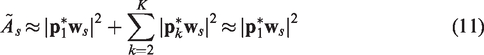
Conventional beamforming^24,25 is a very popular method, since it is robust, fast, and intuitive. Conventional beamforming can be applied using time pressure signals recorded by a set of N microphones, also known as an acoustic array. Usually, a planar acoustic array is used. A scan plane is defined as a set of grid points on a plane at a distance h parallel to the acoustic array. A schematic is shown in Figure 1. With a predefined scan grid, the method works by assuming a potential sound source at each scan grid point and determining its power.

Figure 1.

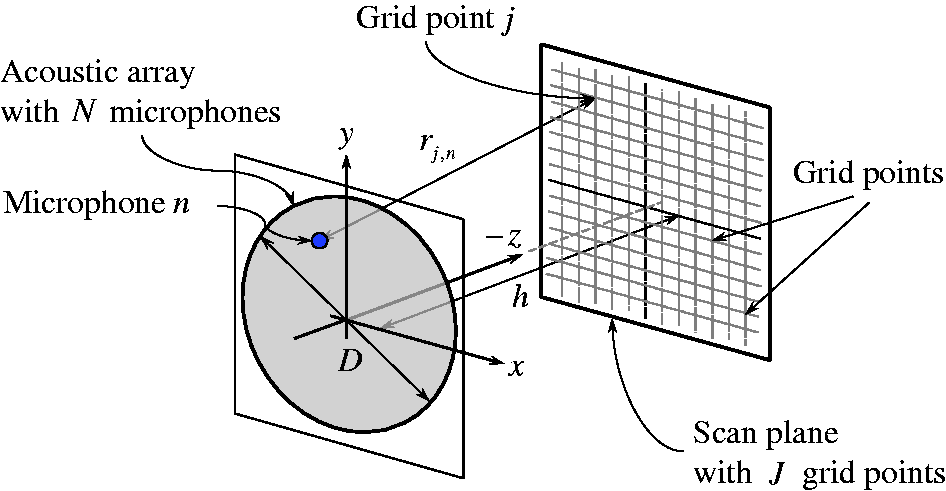
Schematic of an acoustic array depicted as a circular disc with aperture D and a scan plane at a distance h away having J grid points. The array consists of N microphones.

Let ${\mathbf{p}}_{\text{meas}}\in {\mathbb{C}}^{N\times 1}$ be a vector consisting of the Fourier transforms of the measured microphone time signals, the N × N measured Cross-Spectral Matrix (CSM), C_meas, is calculated as

$${\mathbf{C}}_{\text{meas}}=〈{\mathbf{p}}_{\text{meas}}{\mathbf{p}}_{\text{meas}}^{\ast }〉$$

(1)

where $〈·〉$ denotes the time average of snapshots and (⋅)* the complex conjugate transpose. The CSM C_meas is thus calculated by averaging a large number of Fourier-transformed sample blocks.

To perform beamforming, use is made of steering vectors $\mathbf{g}\in {\mathbb{C}}^{N\times 1}$ , which are the modeled complex pressure amplitudes at the microphone locations for a sound source with unit strength at a given grid point. ²⁶ There are several steering vector formulations in the literature, ²⁷ but commonly, the omnidirectional monopole representation is used from the Green’s function of the Helmholtz equation. For microphone n and grid point j, this is given by

$$g_{j,n}=\frac{1}{4\pi r_{j,n}}\exp \left(\frac{-2\pi \mathit{if}{r}_{j,n}}{c}\right)$$

(2)

where f is the frequency of the sound source, c is the speed of sound, i is the imaginary unit, and r_{j, n} is the distance between grid point j and microphone n.

The estimated source power $\tilde{A}$ at grid point j is then given by

$${\tilde{A}}_j={\mathbf{w}}_j^{\ast }{\mathbf{C}}_{\text{meas}}{\mathbf{w}}_j$$

(3)

where w _j is the weight vector ²⁶ given by

$${\mathbf{w}}_j=\frac{{\mathbf{g}}_j}{{\Vert {\mathbf{g}}_j\Vert }^2}$$

(4)

Equation (3) is known as Conventional Frequency Domain Beamforming (CFDBF). To get a source map, equation (3) is applied to a set of grid points.

For CFDBF, the spatial resolution in the source map, given by an acoustic array, is limited by the Rayleigh resolution limit. Assuming plane-wave propagation, the Rayleigh resolution limit is given by

$$\Delta \ell \approx 1.22h\frac{c}{\mathit{fD}}=1.22h\frac{\lambda }{D}$$

(5)

meaning that two sources with a distance less than Δℓ cannot be resolved. From equation (5), it can be derived that the spatial resolution depends on the ratio between the acoustic wavelength λ and the array aperture D, as well as the distance to the scan plane h. Equation (5) shows that Δℓ varies inversely with f.

CLEAN-SC

Apart from the Rayleigh resolution limit, the result of CFDBF is limited by high sidelobe levels, especially at high frequencies. Consequences are that weaker secondary sound sources can be masked by sidelobes of dominant sources. The sidelobe pattern of a source is represented by the Point Spread Function (PSF) of the microphone array, inherent to any imaging system. Knowledge of the PSF allows correction of the image by deconvolution. A common deconvolution method in acoustic imaging is CLEAN-SC. ²⁰ This method is based on the CLEAN method used in astronomy, ²⁸ where deconvolution is performed by assuming the measurement to be exactly proportional to the steering vector g with elements given by equation (2). CLEAN-SC goes a step further by finding the so-called source components h which more closely resemble the measured data contained in p_meas and using the fact that sidelobes are spatially coherent with the main lobe. Both techniques are iterative procedures where source contributions are removed at each step from the CSM and replaced with clean beams in the source map.

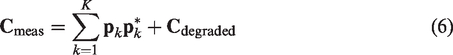
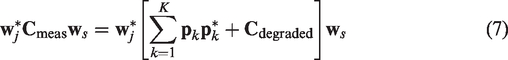
In CLEAN-SC, the measured CSM is decomposed as follows

$${\mathbf{C}}_{\text{meas}}={\displaystyle \sum _{k=1}^K{\mathbf{p}}_k}{\mathbf{p}}_k^{\ast }+{\mathbf{C}}_{\text{degraded}}$$

(6)

meaning that the measured CSM consists of two parts. The first part represents the contribution of K incoherent sound sources. The second part, C_degraded, represents the remaining part in C_meas, where the source information is not (yet) extracted. Herein, p _k are the N-dimensional acoustic source vectors representing the Fourier components of the signals from the kth source. The assumption of equation (6) is valid under the following conditions:

• All sound sources present are incoherent.

• The CSM is calculated from a large number of time blocks, so that the ensemble averages of the cross-products ${\mathbf{p}}_k{\mathbf{p}}_l^{\ast },k\ne l$ , can be neglected.

• There is no decorrelation of signals from the same source between different microphones (e.g. due to sound propagation through turbulence).

• There is no additional incoherent noise.

Let the highest power ${\tilde{A}}_{\text{s}}$ be noted by grid point $s={\text{argmax}}_j({\tilde{A}}_j)$ with the corresponding weight vector w _s , the source power at any grid point j is spatially coherent with this source power peak, ²⁰ or

$${\mathbf{w}}_j^{\ast }{\mathbf{C}}_{\text{meas}}{\mathbf{w}}_s={\mathbf{w}}_j^{\ast }\left[{\displaystyle \sum _{k=1}^K{\mathbf{p}}_k}{\mathbf{p}}_k^{\ast }+{\mathbf{C}}_{\text{degraded}}\right]{\mathbf{w}}_s$$

(7)

At the first iteration step of CLEAN-SC, the exact number of sources K is not yet known, and all information is still contained in C_meas, i.e. C_meas = C_degraded. The CLEAN-SC algorithm extracts the constituting source information from C_meas and transfers it to the first term on the RHS of equation (6). To achieve this, CLEAN-SC starts with the result of CFDBF from equation (3), focusing at the grid point s where the strongest source is identified as

$${\tilde{A}}_s={\mathbf{w}}_s^{\ast }{\mathbf{C}}_{\text{meas}}{\mathbf{w}}_s={\mathbf{w}}_s^{\ast }\left[{\displaystyle \sum _{k=1}^K{\mathbf{p}}_k}{\mathbf{p}}_k^{\ast }+{\mathbf{C}}_{\text{degraded}}\right]{\mathbf{w}}_s$$

(8)

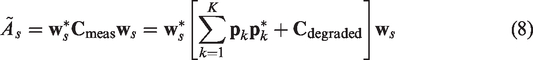
By using the CSM decomposition assumption introduced in equation (6) and expanding the summation term on the RHS of equation (8), assuming that C_degraded is small compared to the part resulting from the contribution of the K incoherent sound sources, i.e. ${\mathbf{C}}_{\text{meas}}\approx {\sum }_{k=1}^K{\mathbf{p}}_k{\mathbf{p}}_k^{\ast }$ , we have

$${\mathbf{C}}_{\text{meas}}{\mathbf{w}}_s\approx ({\mathbf{p}}_1^{\ast }{\mathbf{w}}_s){\mathbf{p}}_1+{\displaystyle \sum _{k=2}^K({\mathbf{p}}_k^{\ast }{\mathbf{w}}_s)}{\mathbf{p}}_k$$

(9)

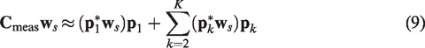
At j = s, it can further be assumed that the second term on the RHS of equation (9), i.e. the contribution from the other sources, is small compared to the first term, and an approximation can be made

$${\mathbf{C}}_{\text{meas}}{\mathbf{w}}_s\approx ({\mathbf{p}}_1^{\ast }{\mathbf{w}}_s){\mathbf{p}}_1$$

(10)

In the same manner

$${\tilde{A}}_s\approx |{\mathbf{p}}_1^{\ast }{\mathbf{w}}_s{|}^2+{\displaystyle \sum _{k=2}^K|}{\mathbf{p}}_k^{\ast }{\mathbf{w}}_s{|}^2\approx |{\mathbf{p}}_1^{\ast }{\mathbf{w}}_s{|}^2$$

(11)

Dividing equation (10) by $|{\mathbf{p}}_1^{\ast }{\mathbf{w}}_s{|}^2$ yields

$$\frac{{\mathbf{C}}_{\text{meas}}{\mathbf{w}}_s}{|{\mathbf{p}}_1^{\ast }{\mathbf{w}}_s{|}^2}\approx \frac{{\mathbf{p}}_1}{\left|{\mathbf{p}}_1^{\ast }{\mathbf{w}}_s\right|}\equiv {\mathbf{h}}_s$$

(12)

assuming that the phase of ${\mathbf{p}}_1^{\ast }{\mathbf{w}}_s$ is irrelevant, and can be written as $\left|{\mathbf{p}}_1^{\ast }{\mathbf{w}}_s\right|$ . The so-called source component, h _s , representing the identified source’s contribution in the measured CSM is now defined. This contribution is to be removed from the measured CSM before proceeding to the next iteration. Equation (11) assumes that the source power at j = s is approximately only the result of one source k = 1. However, there is also a small contribution from the other unidentified sources at j = s.^18,19 Therefore, a safety factor is used to account for their contributions. This is the so-called loop gain, ²⁰ ϕ. As an extension to equation (11), we define

$$|{\mathbf{p}}_1^{\ast }{\mathbf{w}}_s{|}^2=\varphi {\tilde{A}}_s$$

(13)

The loop gain 0 < ϕ ≤ 1 indicates to which extent we assume the source power at grid point s to contain the influence of the identified source k = 1. For example, ϕ is set to 0.99 in this manuscript, meaning that 99% of source power results from the identified source.

Finally, the influence of the source is taken away from the measured CSM by

$${\mathbf{C}}_{\text{degraded}}={\mathbf{C}}_{\text{meas}}-{\mathbf{p}}_1{\mathbf{p}}_1^{\ast }={\mathbf{C}}_{\text{meas}}-|{\mathbf{p}}_1^{\ast }{\mathbf{w}}_s{|}^2{\mathbf{h}}_s{\mathbf{h}}_s^{\ast }={\mathbf{C}}_{\text{meas}}-\varphi {\tilde{A}}_s{\mathbf{h}}_s{\mathbf{h}}_s^{\ast }$$

(14)

yielding C_degraded which replaces C_meas in the next iteration. First, C_degraded replaces C_meas in equation (3) to identify the next source, i.e. the grid point with the source peak. Then the CLEAN-SC process is repeated.

The stopping criterion for CLEAN-SC is when C_degraded is empty after the source components for all incoherent sources have been taken away. In other words, its norm should be sufficiently small compared to the original CSM: $\Vert {\mathbf{C}}_{\text{degraded}}\Vert <\epsilon \Vert {\mathbf{C}}_{\text{meas}}\Vert$ , where ε is a constant here taken as 0.01.

At this point, the exact number of sources K is known. Let the set S contain K indices of grid points where the sources are identified by CLEAN-SC such that s ∈ S, the new source map is obtained by the summation of all the clean beams from the K identified sources and the remaining degraded CSM as

$${\tilde{A}}_j={\displaystyle \sum _{k\prime \in S}\varphi }{\tilde{A}}_{k\prime }{10}^{-\beta d_{j,k^{\prime }}^2}+{\mathbf{w}}_j^{\ast }{\mathbf{C}}_{\text{degraded}}{\mathbf{w}}_j$$

(15)

where β is the clean beam shape parameter and $d_{j,k\prime }$ the distance from grid point j to the identified source location at grid point $k\prime$ .

The CLEAN-SC method results in the improvement of both the MLW and the MSL in the source map. The MSL is lowered by the elimination of sidelobes which are spatially coherent to the main lobe, improving the dynamic range. The MLW is controlled by β and selected by the user, β = 480, in this case. While this can provide smaller beam widths, it does not provide spatial resolution beyond the Rayleigh resolution limit given in equation (5). For sources which are spaced closer than this limit, CLEAN-SC locates the source marker in between.

HR-CLEAN-SC

Having applied CLEAN-SC, the exact value for the number of sources K is determined. The source locations are marked where their peaks are. For HR-CLEAN-SC, the source markers given by CLEAN-SC are relocated such that the relative contribution of the other (K – 1) sources is minimal.^18,19 The new source marker location which matches this requirement for a given source originally marked at s is determined by searching for m which minimizes the cost function as^18,19

$$m={\text{argmin}}_j\left\{F({\mathbf{u}}_j)=\frac{{\Vert {\displaystyle {\sum }_{k^{\prime }\in S,k^{\prime }\ne s}({\mathbf{g}}_{k^{\prime }}^{\ast }{\mathbf{u}}_j)}{\mathbf{g}}_{k^{\prime }}\Vert }^2}{|{\mathbf{g}}_j^{\ast }{\mathbf{u}}_j{|}^2{\Vert {\mathbf{g}}_j\Vert }^2}\right\}$$

(16)

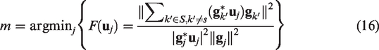
With this, the original weight vector w _s is replaced by u _m , where m associates with a grid point index where the new source marker is to be placed. At this grid point, the total relative contribution of the other sources located at $k\prime \in S,k\prime \ne s$ is minimized.

The choices for the marker location are restricted to a predefined set of J grid points representing the scan plane. Therefore, employing the brute force approach, i.e. evaluating equation (16) for all J grid points, is sufficient to determine u _m in a short time.

The corresponding source component for the new marker u _m then becomes

$${\mathbf{h}}_m=\frac{{\mathbf{C}}_{\text{meas}}{\mathbf{u}}_m}{{\mathbf{u}}_m^{\ast }{\mathbf{C}}_{\text{meas}}{\mathbf{u}}_m}$$

(17)

The corresponding source power estimates for the remaining grid points are calculated by varying ${\mathbf{w}}_j^{\ast }$ to cover the entire scan plane as

$${\tilde{A}}_j=({\mathbf{u}}_m^{\ast }{\mathbf{C}}_{\text{meas}}{\mathbf{u}}_m)|{\mathbf{w}}_j^{\ast }{\mathbf{h}}_m{|}^2$$

(18)

For this map, the maximum ${\tilde{A}}_s$ is determined in the same manner as shown previously, $s={\text{argmax}}_j({\tilde{A}}_j)$ , where j = s represents the actual location of the source. It is important to highlight that, for HR-CLEAN-SC, it is possible that m ≠ s, meaning that the source markers are not necessarily at the source’s peak.

For the next source, C_meas is replaced by C_degraded calculated as in equation (14). Then the process from equations (16) to (18) is repeated for all the remaining sources found in CLEAN-SC until all marker locations and actual source locations do not change anymore, or the maximum number of iterations (20 in this case) is reached. ¹⁸ Finally, the source map is computed using equation (15).

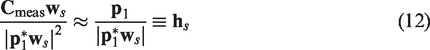
To avoid division by zero in equation (16), a constraint has to be set for any arbitrary source marker u _j as

$$|{\mathbf{g}}_j^{*}{\mathbf{u}}_j{|}^2\ge \mu >0$$

(19)

The parameter μ will be the source marker constraint of the minimization problem in equation (16) and limits how far the source marker is allowed to move from the main lobe’s peak. It is desirable to stay on the main lobe as actual sources might have different PSFs. ²⁰ Therefore, μ should be larger than the MSL. In the work of Sijtsma et al.,^18,19 no improvement in resolution was found for μ below 0.25 for the acoustic array configuration used. Therefore, a constant μ = 0.25 was taken, which is equivalent to 10log₁₀(0.25) ≈ –6 dB relative to the main lobe’s peak.^18,19

Figure 2 schematically illustrates the aforementioned concepts of the HR-CLEAN-SC algorithm. Supposing that there are two closely spaced sound sources placed at a distance d apart, which is lower than the Rayleigh resolution limit (d < Δℓ), these two sources are represented by PSF 1 and 2. Figure 2 shows the resolved two sources with the alternated source marker locations at the final iteration of HR-CLEAN-SC. For PSF 1, the source marker is shifted to the grid point where the influence of PSF 2 is minimized, according to equation (16). The same applies for the source marker of PSF 2. In HR-CLEAN-SC, the source marker is allowed to shift within the source marker constraint μ defined in equation (19).

Figure 2.

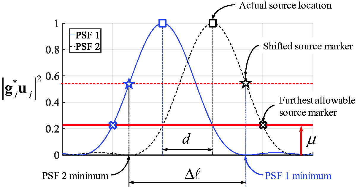
Schematic of two closely spaced sound sources resolved by HR-CLEAN-SC after the source markers have been shifted. The source marker constraint μ is also shown.

Enhanced HR-CLEAN-SC

As mentioned in the previous section, the parameter μ should be larger than the MSL, which strongly depends on the sound frequency considered (f) and the acoustic array design. Hence, an Enhanced version of HR-CLEAN-SC was recently proposed ²³ in order to benefit from the usage of acoustic arrays with low MSL at low frequencies, where μ varies per frequency as

$$\mu (f)={10}^{\text{MSL}(f)/10}$$

(20)

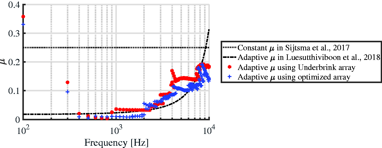
Thus, for a finite predefined scan grid, MSL(f) < 0 is calculated for each frequency of interest as the relative level in dB between the main lobe’s peak and the maximum sidelobe’s peak. As an example, the obtained adaptive values of μ(f) for a range of frequencies, and for the two microphone arrays depicted in Figure 3, are presented in Figure 4, as well as the constant value of μ = 0.25 used by Sijtsma et al.^18,19 as a reference. Moreover, the results for μ(f) assuming that the MSL increases linearly with frequency ²³ are also presented.

Figure 3.

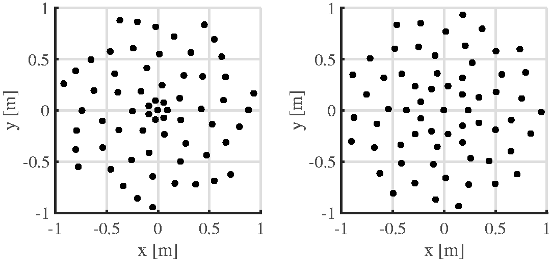
Acoustic arrays used; Underbrink array (left) and optimized array (right).

Figure 4.

Value of μ used in the Enhanced HR-CLEAN-SC algorithm versus frequency to resolve two closely spaced sound sources from synthesized data using the Underbrink and optimized arrays, compared with μ = 0.25 in the HR-CLEAN-SC algorithm ¹⁸ and the adaptive μ based on the assumed MSL. ²³

In practice, evaluating the PSF per frequency is performed as a part of the HR-CLEAN-SC algorithm where the term $|{\mathbf{g}}_j^{*}{\mathbf{u}}_j{|}^2$ , representing the PSF, is evaluated for all J grid points. Therefore, evaluating the exact value of MSL from the already-existing PSF hardly incurs additional computation time compared to HR-CLEAN-SC. However, in case very wide frequency ranges or very fine grids are required, the MSL per frequency can be approximated by empirical formulae ²⁹ to ease the computational effort.

Synthetic data

In this section, the resolvability of up to four closely spaced synthetic sound sources is investigated when the different acoustic imaging algorithms introduced in the previous section are applied. To study the influence of the array design, two acoustic array designs with 64 microphones are used in this study: the multi-arm spiral Underbrink array ³⁰ and the optimized acoustic array designed in a previous study ²³ at Delft University of Technology (TU Delft). The microphone configurations of both arrays are shown in Figure 3.

The simulated sound sources are incoherent point sources emitting white noise. The sources are placed in a plane at a distance h = 1.9 m from the array plane and with separation distance d = 10 cm from each other. The aperture D of both arrays is 1.9 m. With these values, equation (5) states that the sources should be resolved only for f ≥ 4.2 kHz.

For the case of two sources, the calculated sound pressure levels (SPL) of the sources are compared with their exact values for the frequency range from 500 Hz to 10 kHz. Then the source maps at 2 kHz, which is a frequency below the Rayleigh resolution limit, are examined. All the source maps displayed in this paper correspond to narrow-band results, i.e. just at the frequency specified.

Figure 4 shows the values of adaptive source marker constraint μ used to resolve two closely spaced synthetic sound sources by the Enhanced HR-CLEAN-SC algorithm. The value of μ for each frequency is determined by equation (20). This makes μ differ between different arrays as they have different MSLs. Good agreement can be seen between the values of μ determined by the actual MSLs and the approximated values of μ based on the assumed MSLs in previous research. ²³ However, since, for most applications, calculating the PSF and determining the exact MSLs is simple and not time-consuming, it is recommended to derive μ from the exact MSLs. This ensures that the HR-CLEAN-SC algorithm is most efficiently used and the source marker will always stay on the main lobe. It can be seen that μ is almost constant for the optimized array from 400 to 2000 Hz. This is due to the low-sidelobe design of the optimized array. ²³ Nevertheless, the values of μ used by both arrays at higher frequencies are comparable. It is also notable that when the frequency is low, i.e. f ≤ 300 Hz, the value of adaptive μ increases up of more than 0.3. This is because only the main lobe dominates the scan area at low frequency. In this case, the source marker can be moved to any grid point.

Figure 5 shows the offset of the resolved SPL from the exact value versus frequency when CLEAN-SC, HR-CLEAN-SC, and Enhanced HR-CLEAN-SC beamforming are used to resolve two closely spaced synthetic sound sources. Comparison is made between the Underbrink and the optimized array. The offset is shown in terms of ΔSPL = SPL_resolved − SPL_exact. With this, overestimation and underestimation of the SPL are indicated by the positive and negative values, respectively. The two sound sources are correctly resolved when ΔSPL reaches zero. The vertical dashed line indicates f = 4.2 kHz which is the frequency associated with the Rayleigh resolution limit. Above this line, all beamforming algorithms are expected to resolve both sources correctly. It can be seen that the CLEAN-SC algorithm can correctly resolve both sources only above this frequency. The HR-CLEAN-SC algorithm resolves the sound sources from a frequency below the Rayleigh resolution limit, which can be seen as the improvement caused by the HR-CLEAN-SC algorithm. This frequency range is even more widened when the Enhanced HR-CLEAN-SC algorithm is used due to the more flexible selection of source marker locations. The influence of using different acoustic arrays can also be seen in Figure 5. It is shown that the two sources are resolved in the widest range of frequency when the optimized acoustic array is used with the Enhanced HR-CLEAN-SC algorithm, solving both sources for frequencies as low as 1 kHz.

Figure 5.

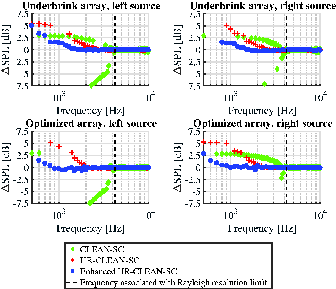
Offset of resolved SPLs of two synthesized sound sources versus frequency by CLEAN-SC, HR-CLEAN-SC, and Enhanced HR-CLEAN-SC beamforming, using the Underbrink and optimized acoustic arrays.

Figures 6 to 8 show the acoustic source maps for two, three, and four synthesized sound sources, respectively. The distance between the neighboring sources is d = 10 cm. The source maps are produced by CFDBF, CLEAN-SC, HR-CLEAN-SC, and Enhanced HR-CLEAN-SC, using the Underbrink and optimized acoustic arrays at 2 kHz. The exact locations of the sources are denoted by the dashed line intersections. For two sources, it has already been anticipated from Figure 5 that the sources are completely resolved by both the Underbrink and the optimized arrays when the Enhanced HR-CLEAN-SC algorithm is used. The source maps in Figure 6 confirm this. However, source resolvability is expected to be more challenging when there are more than two sources. It can be observed that although the HR-CLEAN-SC algorithm can somewhat resolve the three and four sound sources, the source localization is still inaccurate. This feature is improved by the Enhanced HR-CLEAN-SC algorithm. The influence of the acoustic array selection can still be noticed in this case. According to the source maps, the sound sources are most clearly distinguished and most accurately localized when the optimized acoustic array and the Enhanced HR-CLEAN-SC algorithm are used at the same time.

Figure 6.

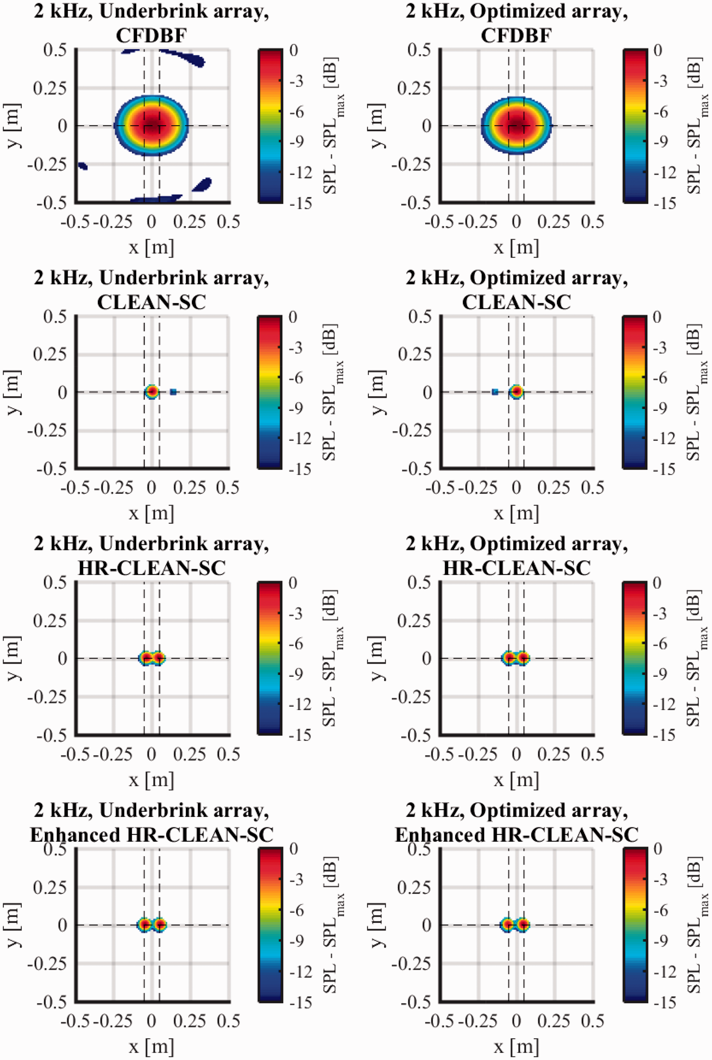
Source maps of two synthesized sound sources with 10 cm separation produced by CFDBF, CLEAN-SC, HR-CLEAN-SC, and Enhanced HR-CLEAN-SC, using the Underbrink and optimized acoustic arrays at 2 kHz.

Figure 7.

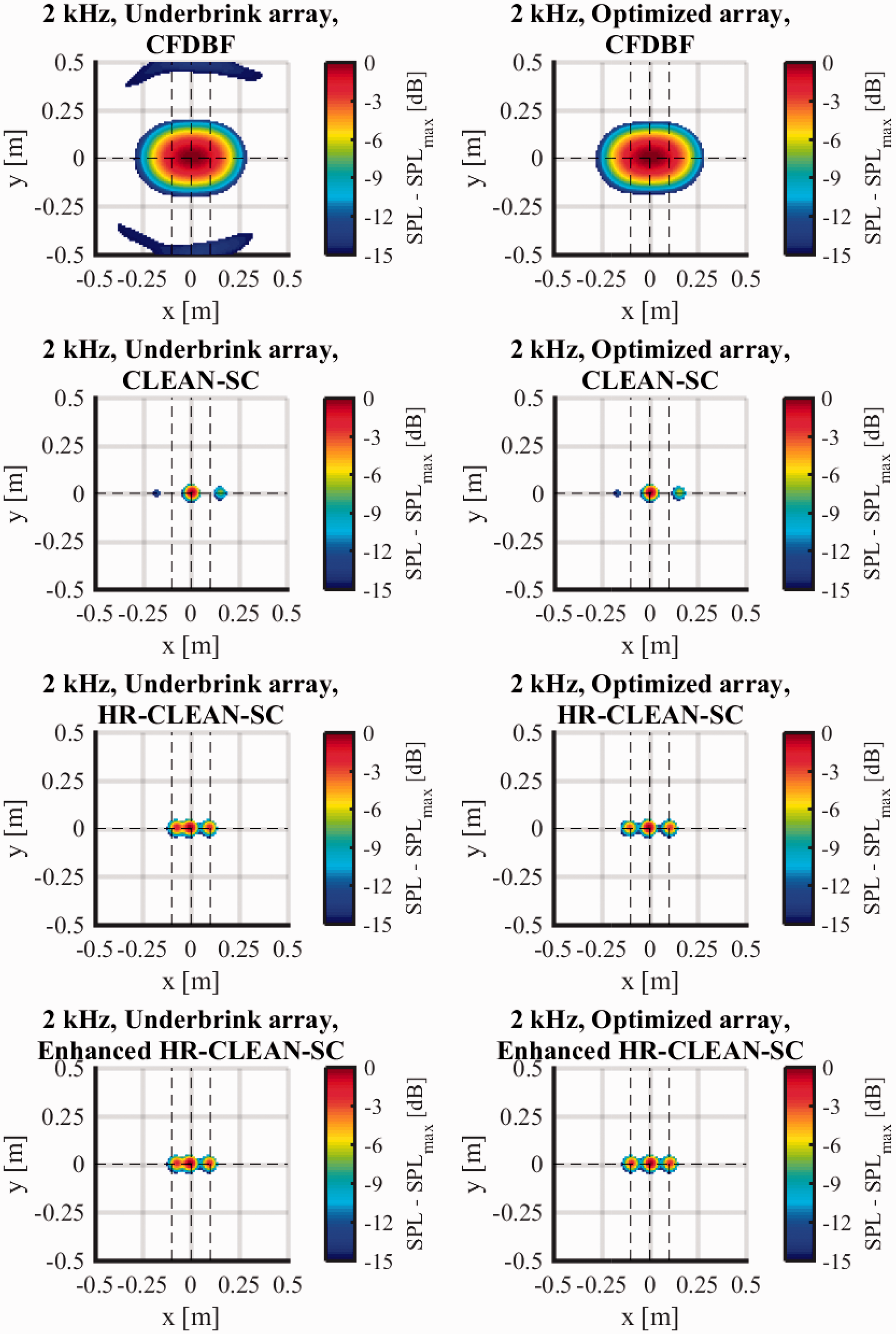
Source maps of three synthesized sound sources with 10 cm separation produced by CFDBF, CLEAN-SC, HR-CLEAN-SC, and Enhanced HR-CLEAN-SC, using the Underbrink and optimized acoustic arrays at 2 kHz.

Figure 8.

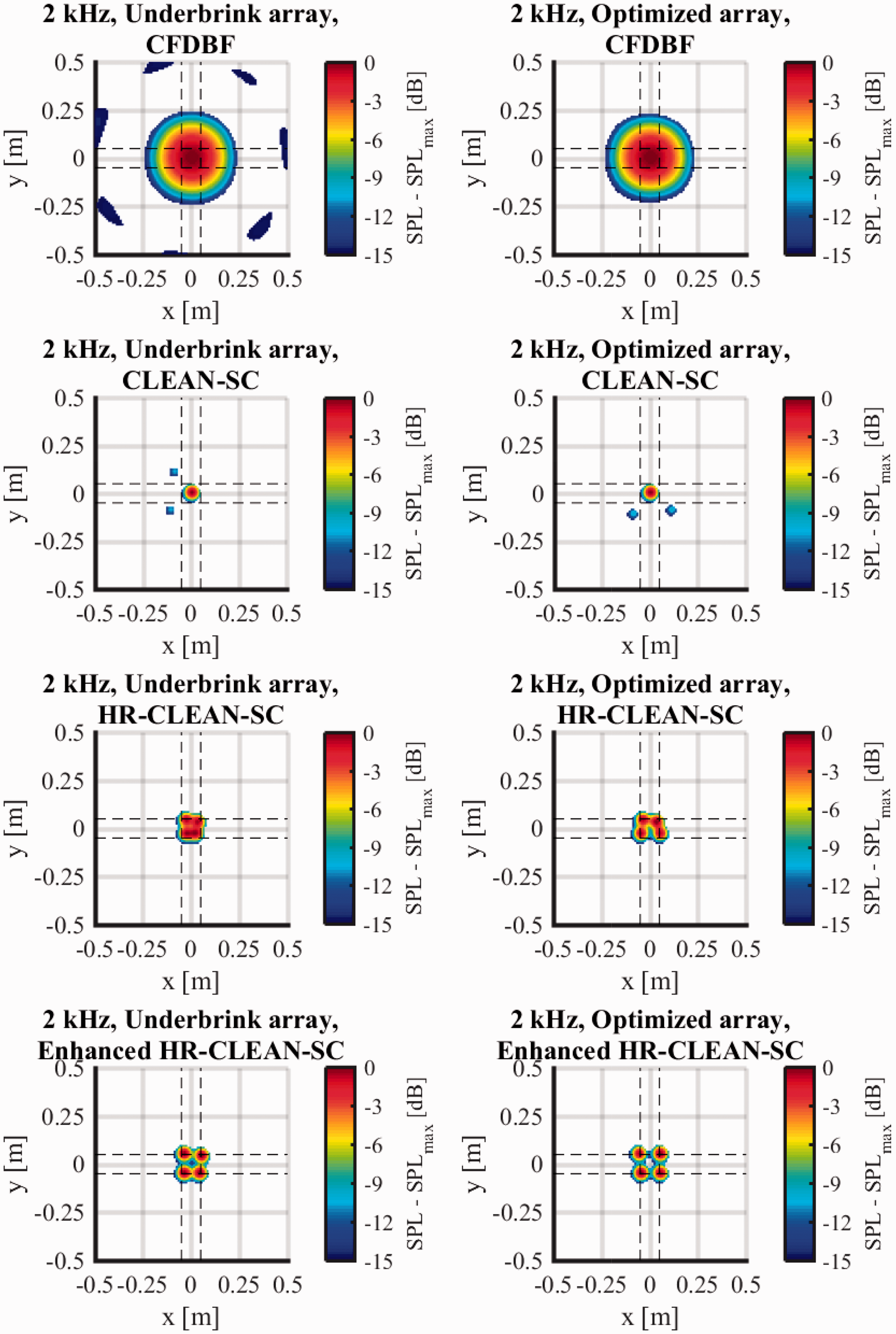
Source maps of four synthesized sound sources with 10 cm separation produced by CFDBF, CLEAN-SC, HR-CLEAN-SC, and Enhanced HR-CLEAN-SC, using the Underbrink and optimized acoustic arrays at 2 kHz.

Experimental validation

The experiments were performed at the anechoic vertical wind tunnel (A-tunnel) at TU Delft, normally used for aeroacoustic experiments.^31–33 The overview of the test setup is shown in Figure 9. The microphone distributions shown in Figure 3 were obtained using 64 G.R.A.S; 40PH microphones installed on a 2 × 2 m perforated steel plate ³³ with an aperture of 1.9 m. The x–y coordinates of the microphones were assigned to the closest holes on the perforated plate. Visaton K50 SQ speakers were used as sound sources. They were placed on a plane located at the distance h = 1.9 m parallel to the array plane and aligned with the array center. Incoherent white noise signals generated by a MATLAB program were fed to the speakers. A unique signal was used for each speaker such that the signal emitted by an individual speaker is different from one another, yet the same set of signals as well as speaker-signal assignment was used throughout the tests. In this way, the results from different cases are fully comparable.

Figure 9.

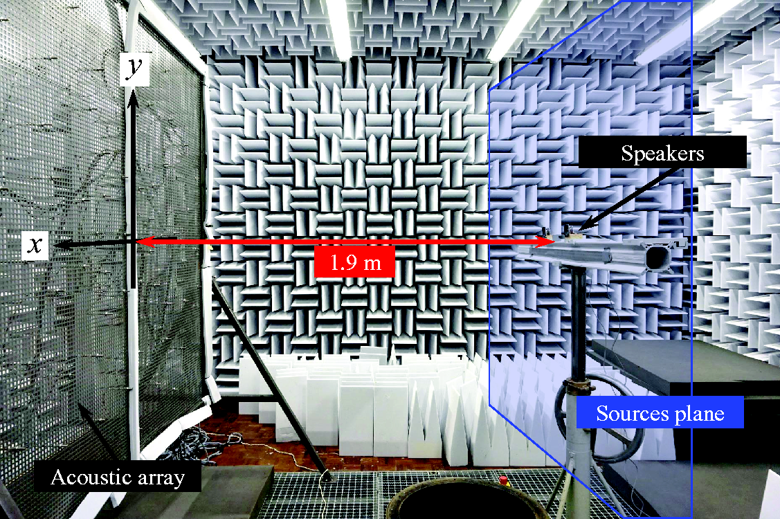
Overview of the experimental setup in the A-tunnel at TU Delft.

The speakers were arranged in two different configurations. First, two speakers were placed at a distance d = 10 cm measured from the center of one speaker to the other. Secondly, five speakers were placed adjacent to each other. Figure 10 illustrates the two configurations together with the speaker number. To achieve the cases where there are two, three, and four closely spaced sound sources, the speakers were operated as follows:

Figure 10.

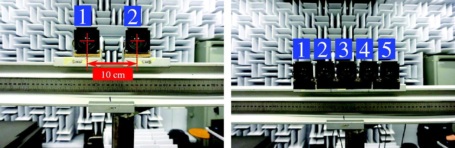
Speaker configurations used; two-speaker configuration (left) and five-speaker configuration (right). The numbers indicate the speaker numbers.

1. Two sources: Using the two-speaker configuration (same setup as in Figure 6).

2. Three sources: Using the five-speaker configuration and playing the signal using speakers 1, 3, and 5.

3. Four sources: Using the five-speaker configuration and playing the signal using speakers 1, 2, 4, and 5.

Apart from playing the signals with multiple speakers simultaneously, recordings were also made when each individual speaker played the signal. With this, the individual contribution of each speaker can be examined and the exact SPL of each speaker can be resolved.

For each recording, the duration of the signal was 30 s. The sampling frequency of the data acquisition system was 50 kHz. The length of the time blocks used in the Fourier transform to produce the time-averaged vector p_meas was a snapshot of 0.01 s (500 samples). The snapshot length used was an arbitrary choice. The snapshot length was also varied such that up to 10 times higher frequency resolution was obtained, i.e. 10 times longer snapshot. However, no notable influence on the results was found. A Hanning weighing function with 50% overlap was applied to each snapshot.

Figure 11 shows the SPL offset (ΔSPL) versus frequency for the case with two closely spaced speakers when the CLEAN-SC, HR-CLEAN-SC, and Enhanced HR-CLEAN-SC algorithms are employed. Again, comparison is made between the Underbrink and the optimized arrays. In the same manner as observed in Figure 5, the CLEAN-SC algorithm resolves both speakers only at the frequencies above those associated with the Rayleigh resolution limit. However, the differences between the HR-CLEAN-SC and the Enhanced HR-CLEAN-SC algorithm, as well as the differences between the two acoustic arrays, cannot be seen as clearly as in the synthetic data case. For this two-speaker case, the sound sources are found to be resolved by both the HR-CLEAN-SC and Enhanced HR-CLEAN-SC methods, and by both arrays, from approximately 2 kHz. This is confirmed by the four lower source maps in Figure 12.

Figure 11.

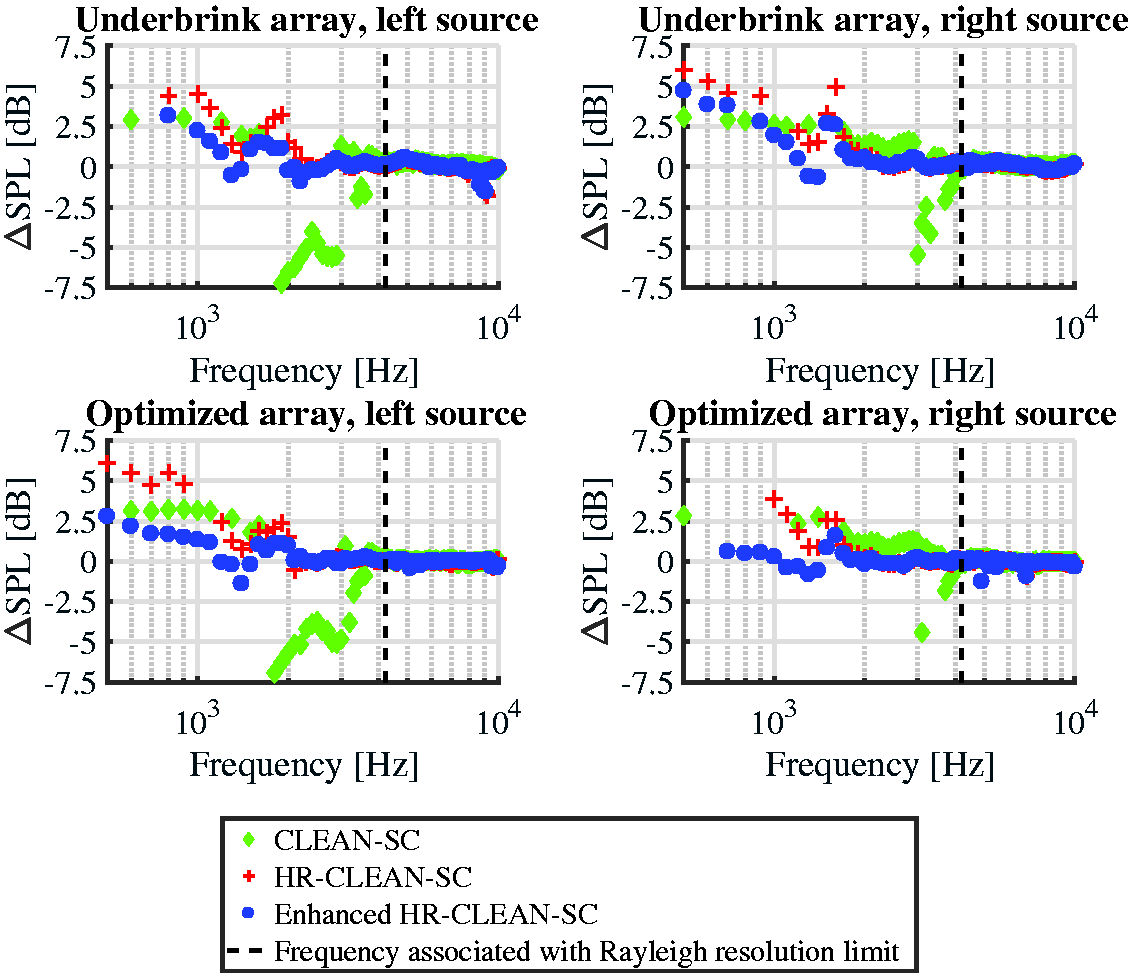
Offset of resolved SPLs of two closely spaced speakers versus frequency by CFDBF, CLEAN-SC, HR-CLEAN-SC, and Enhanced HR-CLEAN-SC, using the Underbrink and optimized acoustic arrays.

Figure 12.

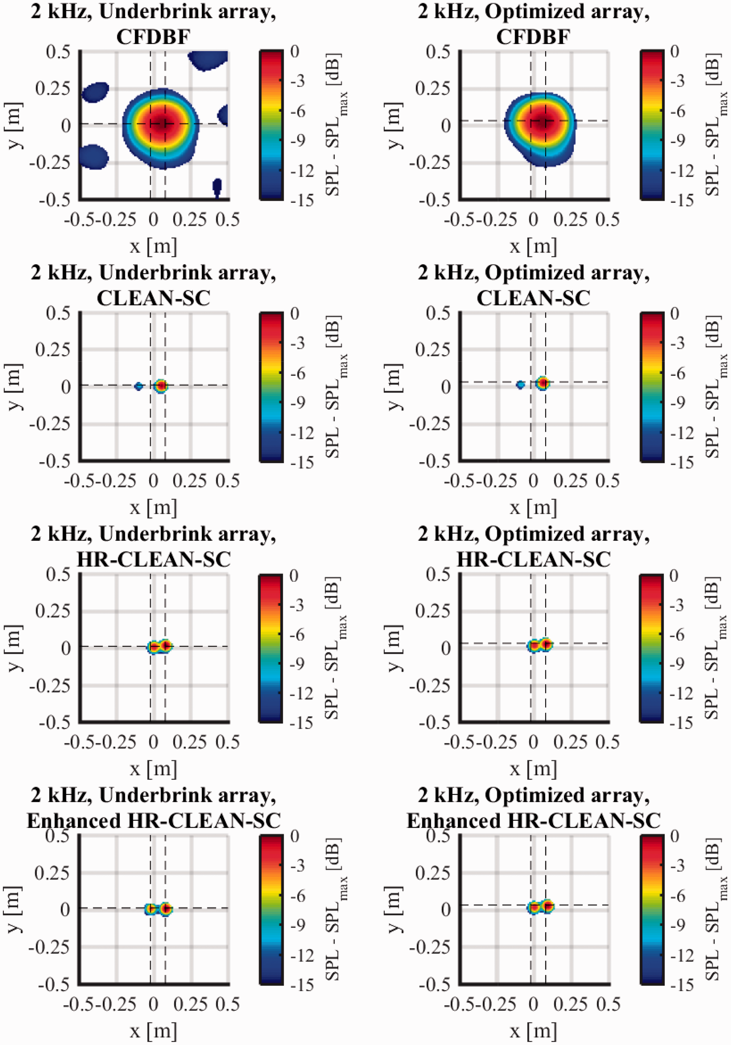
Source maps of two closely spaced speakers produced by CFDBF, CLEAN-SC, HR-CLEAN-SC, and Enhanced HR-CLEAN-SC, using the Underbrink and optimized acoustic arrays at 2 kHz.

Figures 13 and 14 show the source maps from the three and four closely spaced speakers, respectively. The source maps are obtained using CFDBF, CLEAN-SC, HR-CLEAN-SC, and Enhanced HR-CLEAN-SC, using both acoustic arrays. It is important to note that, for these two cases, the distance between the centers of the neighboring speakers d is no longer 10 cm, but instead d = 11 cm for the three-speaker case and d = 5.5 cm for the four-speaker case. Therefore, the frequency at which the source maps are compared should be adjusted to maintain approximately the same level of source discrimination challenge. The selected frequencies are calculated based on equation (5). Subsequently, the source maps in Figures 13 and 14 are shown at 1.8 and 3.6 kHz, respectively. In most cases, the correct number of sources can be recognized when the HR-CLEAN-SC algorithm is used. However, some closely spaced sources are not clearly distinguished and this localization is still inaccurate. This is somewhat improved when the Enhanced HR-CLEAN-SC algorithm is employed. In addition, the selection of the acoustic array also plays a role. The clarity of the source’s boundary and the localization accuracy can be seen more clearly in the case of optimized array.

Figure 13.

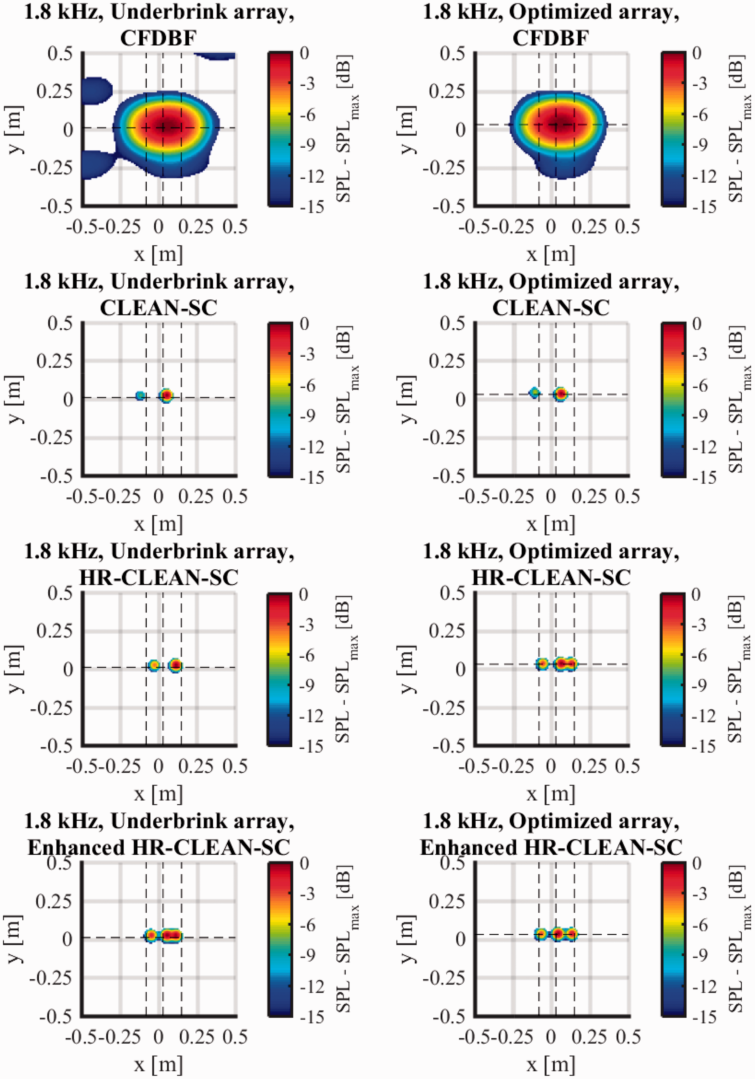
Source maps of three closely spaced speakers produced by CFDBF, CLEAN-SC, HR-CLEAN-SC, and Enhanced HR-CLEAN-SC, using the Underbrink and optimized acoustic arrays at 1.8 kHz.

Figure 14.

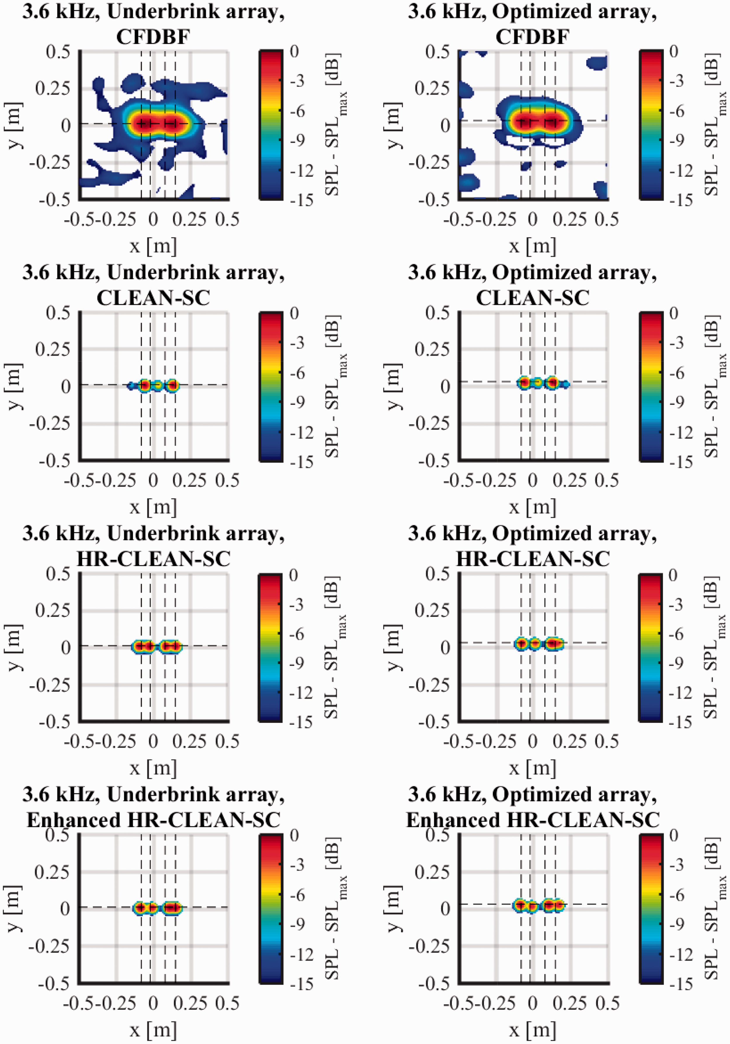
Source maps of four closely spaced speakers produced by CFDBF, CLEAN-SC, HR-CLEAN-SC, and Enhanced HR-CLEAN-SC, using the Underbrink and optimized acoustic arrays at 3.6 kHz.

Conclusions

In this paper, the performance of the deconvolution acoustic imaging methods, CLEAN-SC, HR-CLEAN-SC, and Enhanced HR-CLEAN-SC, is assessed with respect to their ability to distinguish and reveal multiple closely spaced sound sources.

The recently introduced HR-CLEAN-SC algorithm provides super-resolution, i.e. the ability to resolve sound sources placed closer than the Rayleigh resolution limit, while requiring a relatively short computation time. This is done by shifting the source marker to a location where the summation of the relative contributions from the other sources is minimized.

The source marker relocation is regulated by the source marker constraint μ, which is defined to avoid the side lobes in the acoustic array’s point spread function (PSF). This makes the performance of the HR-CLEAN-SC algorithm dependent on the quality of the acoustic array design. The Enhanced HR-CLEAN-SC algorithm has been proposed to exploit the low-sidelobe design of the optimized array. It works by adapting the value of μ with respect to the maximum sidelobe level (MSL) in the array’s PSF for each frequency. This is beneficial since the MSL is normally low at low frequencies, allowing a lower μ to be selected, and, therefore, a more flexible selection of the source marker location, which leads to a maximized resolution improvement.

The results from synthetic data showed that, for up to four closely spaced incoherent sound sources having the frequency associated with the Rayleigh resolution limit of 4.2 kHz, the sources can be discriminated from 2 kHz, when the optimized array is used in combination with the Enhanced HR-CLEAN-SC algorithm. It has also been observed that, for a fixed frequency, source discrimination becomes more challenging as the number of sources to be resolved increases. This can be expected because the feasible region with a low combined influence of the other sound sources, where an alternative location for the source marker of a certain sound source can be placed, gets smaller when there are more sound sources clustering together.

Through experimental validation, the differences between the HR-CLEAN-SC and Enhanced HR-CLEAN-SC as well as between the Underbrink and the optimized acoustic arrays in discriminating two closely spaced speakers are confirmed, but the differences are less pronounced. However, in most cases, when the number of sources increases, the optimized array and the Enhanced HR-CLEAN-SC provide source maps with the clearest source discrimination and the most accurate source localization. Therefore, this combined effect of optimized array geometry and Enhanced HR-CLEAN-SC is recommended.