
Abstract
In this study, an integrated model is developed for studying the Sanchi oil spill event, which occurred in the East China Sea in January 2018. The results of the Advanced Research Weather Research and Forecasting model (WRF-ARW) as well as the Princeton Ocean Model (POM) are used for meteorological forecasting and the hydrodynamic simulations, respectively. These data are adopted as inputs for the OpenOil, a sub-module of OpenDrift, for the oil spill model. Some reference experiments are examined for short-term hindcast. The satellite image is used to validate the numerical result. The oil slicks of the satellite image and the numerical result are of similar shapes. Quantitatively, the simulated oil slick and that from the satellite image are located closely and have similar dimensions of 56 km by 34 km and 54 km by 29 km, respectively. It is found that the accurate results can be obtained by the proposed integrated model with the high-frequency (hourly) and high-spatial-resolution data as inputs, and the wind drift factor has to be added. The long-term 1-month simulation showed that most of the oil particles would move to the northeast of the sinking location and be trapped by the Kuroshio current.
Introduction
Most of the oil spills in the ocean are the results of human activities, for example, marine oil transport, well blowouts, etc. Any spill can cause significant effects on the ecology, economy, and society. Tanker accident, which may lead to a large-scale oil spill, is a considerable concern. To be one of the worst oil spill in US, the Exxon Valdez spilled 42 million liters of crude oil into Prince William Sound, Alaska on March, 1989, that killed a lot kinds of animals, such as sea birds, otters, seals, bald eagles and whales. 1 The total economic loss from this oil spill was estimated to be approximately $2.8 billion as some reports. About 30,000 tons of oil was spilled from the Tasman Spirit when it broken into two parts in July 2003, and the impacts on the environment, public health, and local economy were recorded. The large spills not only cause a tremendous amount of money in damages but also in cleanups. Although the statistical data from the International Oil Tanker Owners Pollution Federation Limited (ITOPF), large and medium (>7 tons) spills show a noticeable downward trend, the growth in the volume of oil transported and in accident rates could lead to more spills related to tankers in the future. 2
On 6 January 2018, the oil tanker Sanchi, with 136,000 tons of ultralight crude oil and about 1900 tons of its fuel oil, crashed into a bulk freighter, the CF Crystal, in the East China Sea, 160 nautical miles off Shanghai, China. It caught fire and went down 8 days later, causing the death of all 32 members of its crew and the discharging of a significant amount of petroleum products. The severe damage to the ecosystem of the East China Sea, which is one of the most heavily trafficked waterways of the world, is inevitable. This area is not only a spawning ground for some species such as blue crabs and hairtails but also on the migratory route of no less than three species of whales. The New York Times stated that this accident could be compared with the Exxon Valdez oil spill. The prediction of oil spill tracking is one of the critical points to protect the environment and assess pollution. It is obvious that numerical models can play an important role for a fast and informed decision-making. It can be used to generate safe and accurate spill scenarios so that it is the ideal tool for not only contingency planning, but also response training, and damage assessments.
The last three decades witnessed the evolution of spill models and their application in supporting spill response and impact assessment. 3 Most of the early models are two-dimensional and can simulate a few processes. 4 These often were given to an easier, but less accurate approach. Nowadays, the better knowledge of oil transport and fate of spilled oil, the improvements in atmospheric and ocean models which provide more accurate model inputs for oil spill models; and the development of computer enable spill models to produce complicated simulations efficiently. Currently, there are more fifteen models widely used and their characteristics are compared. 5 Additionally, many research groups or individual researchers have been developing fate and trajectory model codes for in-house use, without publishing a software code.
Examples of oil spill model include ADIOS, GNOME, SLROSM, GULFSPILL, MOTHY, OILMAP (also with SARMAP), SIMAP, OSCAR, MEDSLIK, MEDSLIK-II, PO-SEIDON-OSM, OILTRANS, SEATRACK WEB, DELFT3D-PART. However, most of them are commercial software, so the source code is unavailable to users for modification and improvement. Therefore dynamic oil spill models have been developed to predict oil behavior over time and are being used as a tool for decision-makers in actual and fictitious spills. The development in computer power and storage has made it possible to integrate many data sources in the simulations, for example, wind, wave, current, water temperature, physical and chemical properties of the oil. Developing an integrated model that has comprehensive algorithms for oil fate and trajectory and open-source code facilitating modification is being of primary interest.
In this study, the transport and fate of oil spill are predicted based on the Advanced Research Weather Research and Forecasting model (WRF-ARW) for the meteorological forecast, the Princeton Ocean Model (POM) for the hydrodynamic simulation in cooperate with the OpenOil, a sub-module of the OpenDrift, for the oil spill model. The OpenDrift is programed in Python and developed at the Norwegian Meteorological Institute. Until now, it includes an oil drift model, a pelagic egg model, a stochastic search and rescue model, and a basic module for atmospheric drift. As open-source code, it is flexible and easy for researchers to adapt or add modules for their specific purpose. The OpenDrift can be set up and used quite fast and simple on Mac, Linux, and Windows environments. 6 These models are publicly available so that the source code and results can be exchanged easily between multiple working groups for better collaboration and verification. The focus of this paper is the application of the proposed integrated model for the Sanchi incident, which is an example of a tanker accident with a huge spilled oil amount in the open sea.
The organization of this paper is listed in the following. The integrated model is introduced in Section 2. Then the Sanchi incident, the simulations of wind and current, as well as the short-term long-term hindcasts are followed in Section 3. Some sensitivity experiments related to the different frequency and spatial resolution models are examined, and the results are validated against the satellite image. The conclusions are presented in Section 4.
Materials and methods
Meteorological forecast model
In the proposed model, the WRF-ARW, a non-hydrostatic model for compressible flow, is used as the meteorological forecasting (Figure 1). The details of this model are available in the UCAR public website. 7
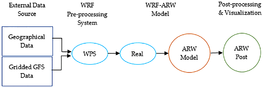
Flowchart for the WRF-ARW modeling system.
The simulations of WRF-ARW start with the WRF Pre-processing System (WPS). Its main functions are to set up the model domain; to interpolate terrestrial data including topography, land use, and reformat and interpolate meteorological data from another model as the input to this model domain. The major program of the system is the dynamical solver, naming the ARW core. Its input is from the initialization unit, and the output is given to the post-processing and visualization. The model uses a mass-based terrain-following hydrostatic pressure vertical coordinate. The grid staggering is the Arakawa C-grid. The reanalysis data of the Global forecast system (GFS) of the National Centers for Environmental Prediction (NCEP) is used as the initial and boundary condition.
The ocean model
The ocean current is simulated by the Princeton Ocean Model, POM. 8 The POM is a free surface, primitive equation circulation numerical ocean model that can be used to simulate the ocean currents, the temperature, the salinity, and other water properties. In the horizontal, the curvilinear orthogonal coordinate is implemented to fit the irregular shoreline boundaries and bottom configurations. In the vertical direction, a sigma coordinate is scaled on the water column depth. The model splits computations between internal mode (for the vertical structure equations) and external mode (the vertically integrated equations). The internal mode is three-dimensional and responsible for updating the velocity, temperature, salinity, and the turbulence quantities. The two-dimensional external mode updates the surface elevation and vertically averaged velocities and computes time-averaged quantities for use in the internal mode. The details of the model code can be found on its public website.
The POM has been used in a wide range of applications. It is a feasible tool for simulating the mixing processes and circulation in the coastal, 9 rivers,10,11 estuaries,12,13 shelves,14,15 lakes,16,17 semi-enclosed seas,18,19 open and global sea.20,21 It also has applied successfully to study many processes of geophysical fluid dynamic.22–26 Moreover, a variety of ocean and coastal forecasting system use this model. Examples include the Advanced Taiwan Ocean Prediction System, 27 the Japan coastal ocean prediction, 28 the Mediterranean Sea forecasting system, 29 etc. The surface currents obtained by the POM are compared against the geostrophic current calculated from the satellite sea surface height (SSH) of AVISO. 30 Here, the SSH contains the mean dynamic topography (MDT) and the sea surface height anomaly (SSHA).
Oil spill model
The oil spill modeling is performed using the OpenOil, which is a module of the generic framework, OpenDrift. This model is programed in Python and was developed at the Norwegian Meteorological Institute. 6 The OpenOil is a Lagrangian trajectory model, in which the spilled oil on sea surface is simulated as a large amount of small particles of equal mass under the influence of velocity fields as parts of oceanic and atmospheric circulations. Spilled oil particles drift in the horizontal direction under the combined action of the ocean current, wave-induced Stokes Drift, and an additional factor of 3.5% of the wind. 31 With regard to vertical movement, three processes are considered:
First, the entrainment rate (

In this equation,
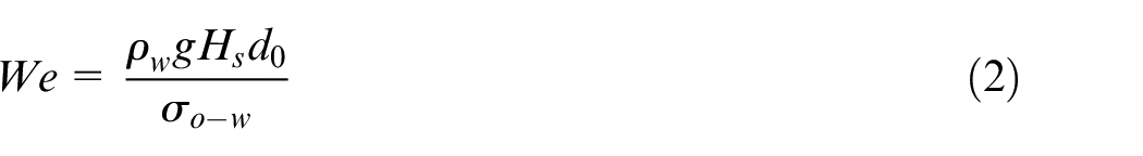
where
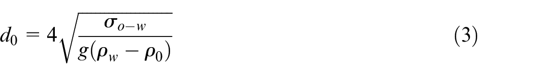
The ratio of viscous forces to inertial and surface tension forces are described by the Ohnesorge number as
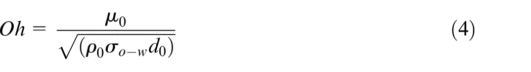
where
The fraction of the sea surface covered by breaking waves per time unit,
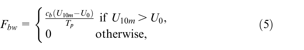
where
The second process is rise or resurfacing of submerged particles due to buoyancy. This process is affected by the droplet size, seawater viscosity, and the density difference between seawater and oil. The terminal vertical rise velocity is given by Tkalich and Chan 35 as follow:
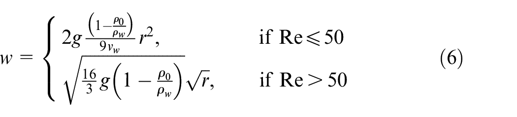
where
The last process is the upwards or downwards turbulent mixing of the submerged oil droplets. This process is simulated by using the random walk scheme. 36
In this work, the time steps for the vertical processes and for the horizontal advection are 10 s and 10 min, respectively. Besides the vertical and horizontal transport, the weather processes, such as evaporation, emulsification, and dispersion, are also modeled as described in Röhrs et al. 34
Overall, the flow chat of the proposed integrated model is shown in Figure 2. In the figure, it is noticeable that the ocean current data from the Hybrid Coordinate Ocean Model (HYCOM) are used as the boundary condition for the ocean model POM. And the wind data from either the WRF-ARW or the NCEP are used to drive the ocean model POM. In the last, the ocean current data and the wind data are used to drive the oil spill model OpenOil.
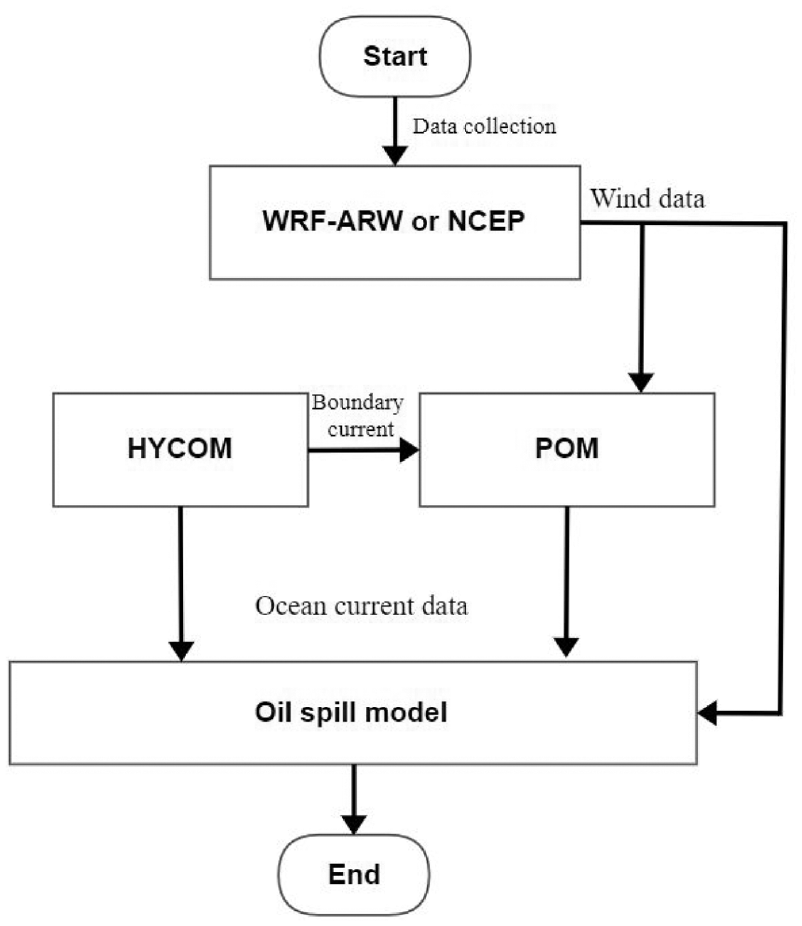
The flow chart of the proposed integrated model.
Hindcast experiments of the Sanchi event
The incident
The oil tanker Sanchi, carrying 136,000 metric tons of condensate oil heading to South Korea from Iran, collided with the cargo ship CF Crystal 160 nautical miles (300 km) off Shanghai, China, on 6 January 2018. Eight days later, on 14 January, at the location about 151 nautical miles away from the collision site, Sanchi sank, and about 1900 tons of fuel oil was spilled out. The site location is depicted in Figure 3.
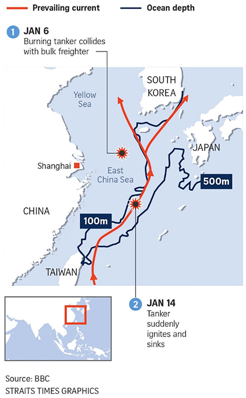
Grounding site of Sanchi event.
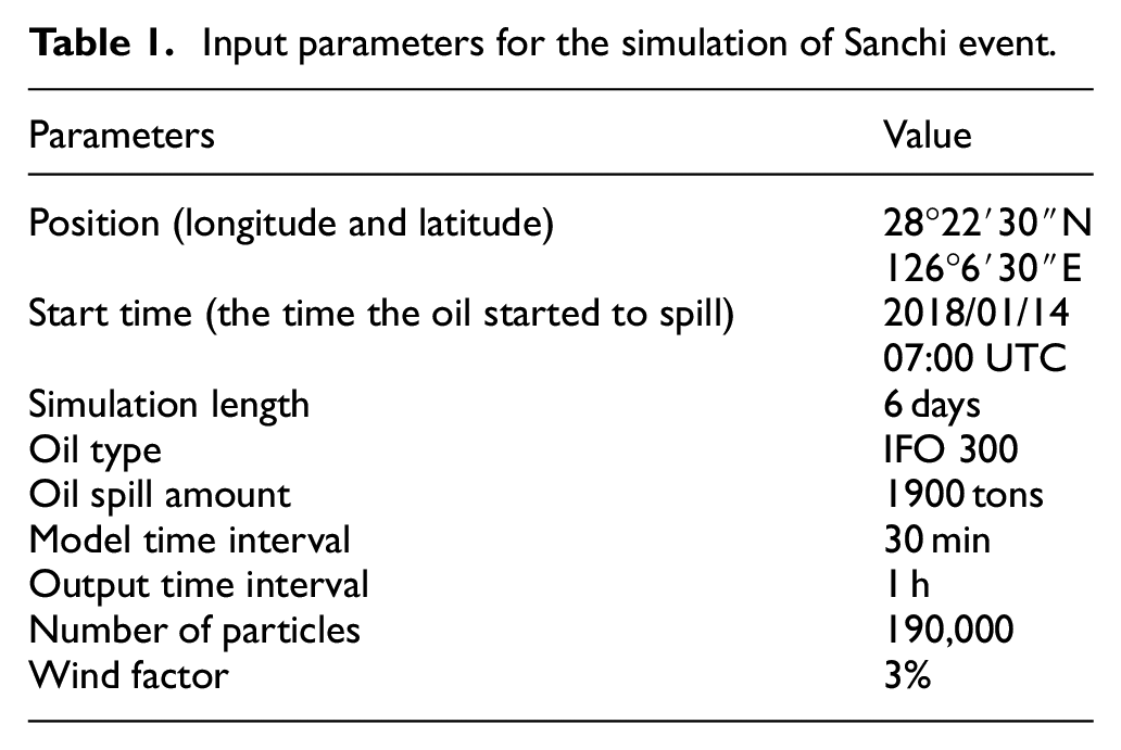
The collision originally occurred on the border between the Yellow Sea and East China Sea, where has complex, strong, and highly variable surface currents. In addition, the sinking site is closer to the edge of the East China Sea, which dominated by the Kuroshio Current as reported by the NOC . 37 The input data are summed up in Table 1.
Input parameters for the simulation of Sanchi event.
Simulation of the wind field
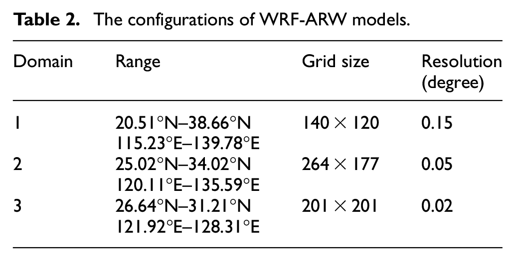
In this study, a triple-nested simulation scheme has developed for the high-resolution forecast on wind fields. The first layer of the nested model is designed with a coarse grid (0.15°) to model the domain of East China Sea. Then, we consider the second layer of the nested area to be with higher grid resolution (0.05°). Lastly, the third one is with the highest grid resolution (0.02°) to model the meteorological condition over the focus areas around the incident location in short-term prediction. The detailed configurations of these models are shown in Table 2. Figure 4 shows the triple-nested domains used in this study. Figure 5 shows wind barb plots of the mean wind field changes in the period of 6 days from 14 to 20 January 2018. In the figure, the orientation of wind barb shows wind direction. The end of barb represents the magnitude of wind with
The configurations of WRF-ARW models.
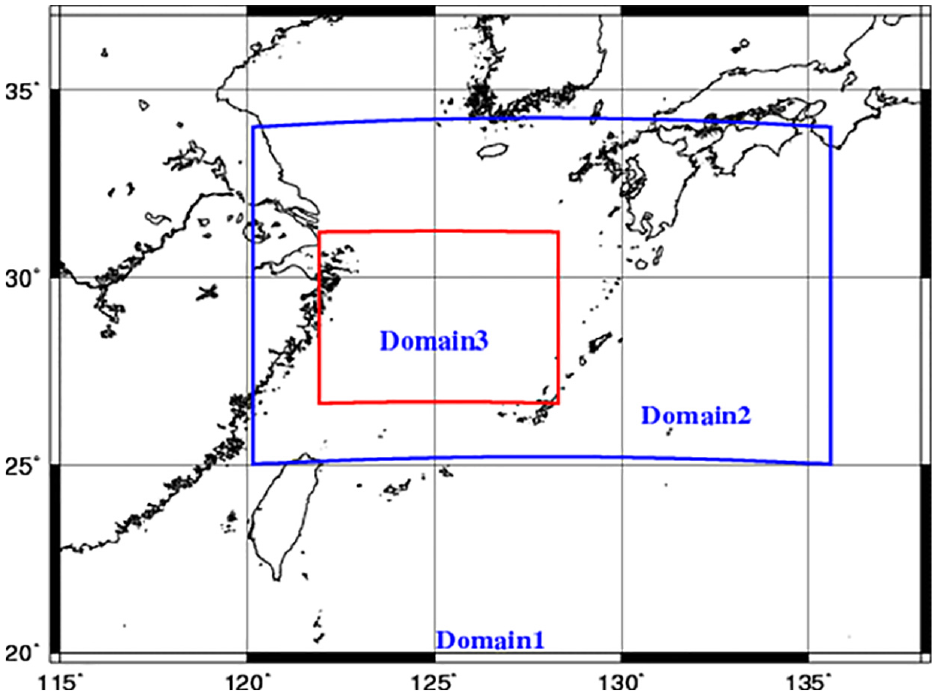
WRF-ARW model the triple-nested domains over the East China Sea.
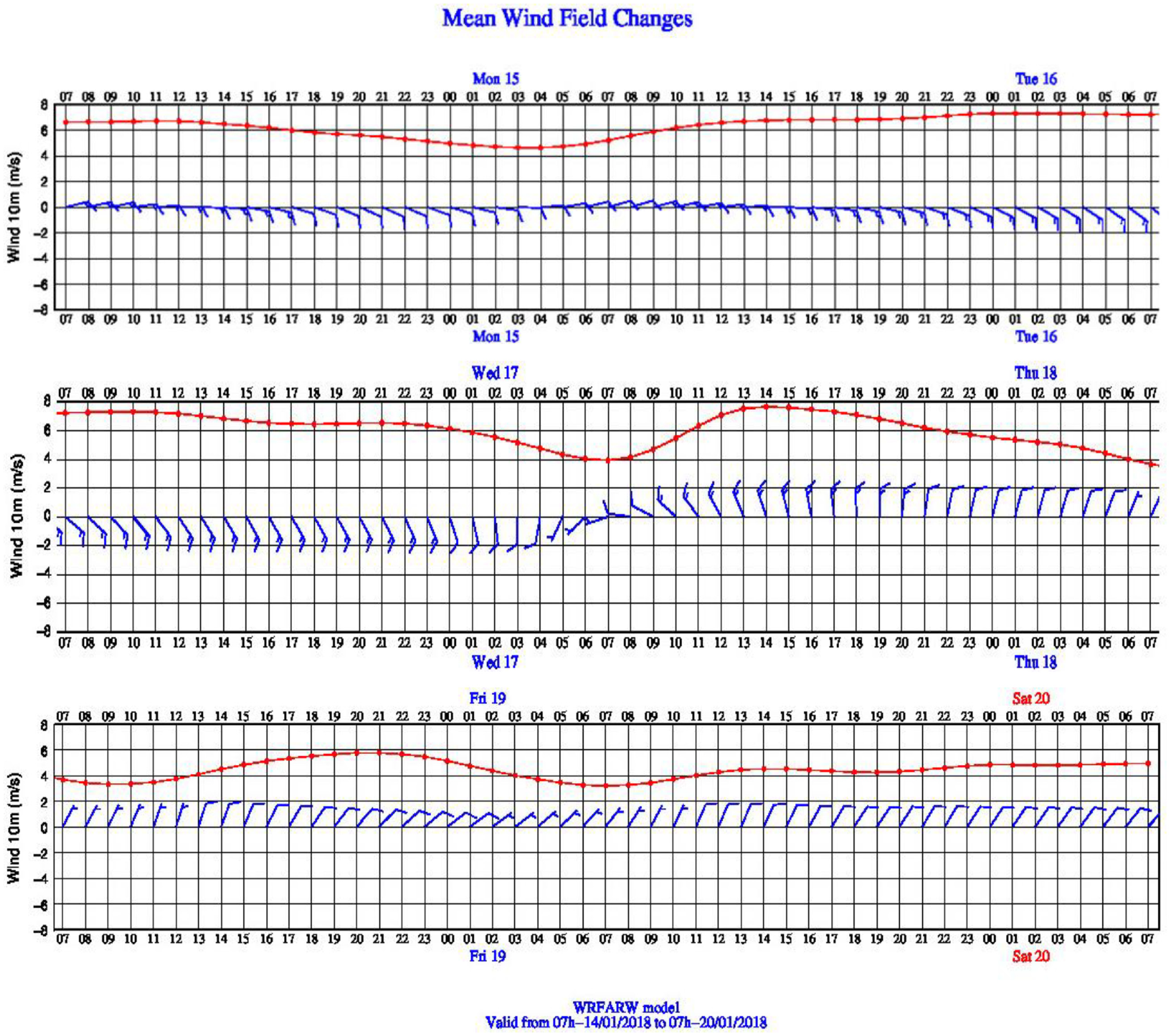
Mean wind field changes from 14 January 2018 07:00 to 20 January 2018 07:00.
Simulation of the Kuroshio current
In order to drive the oil spill model OpenOil, the current data in the considered domain are required. Figure 6 depicts the bathymetry of the study area in the East China Sea. In this study, the current field during the Sanchi event are either modeled by the POM with a grid resolution of 1/25° or adapted from the HYCOM data. The detailed configurations of these ocean models are shown in Table 3. Both the sea surface height and the vertical velocity field are required in the hindcasts. For example, Figure 7(a) shows the computational Kuroshio current from POM on 15 January, 2018 at 7:00. In order to validate the prescribed results, Figure 7(b) depicts the geostrophic current and sea surface height (SSH) calculated from the satellite data of AVISO 30 for comparison. Good agreements between the current data obtained from the POM and the AVISO can be observed. The location of the main eddy and the corresponding current magnitude are significant for both of the results.
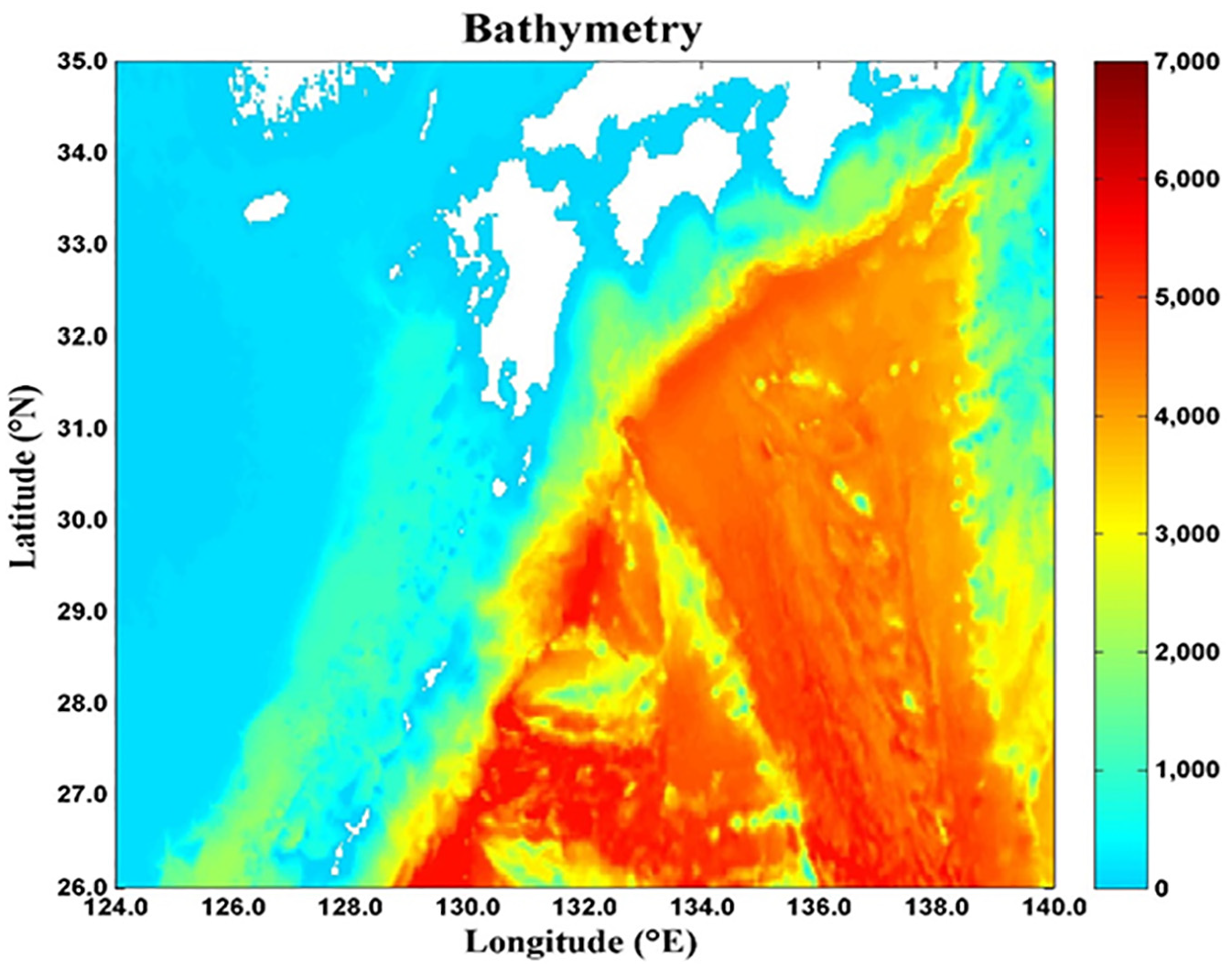
Bathymetry of the incident grounding site.
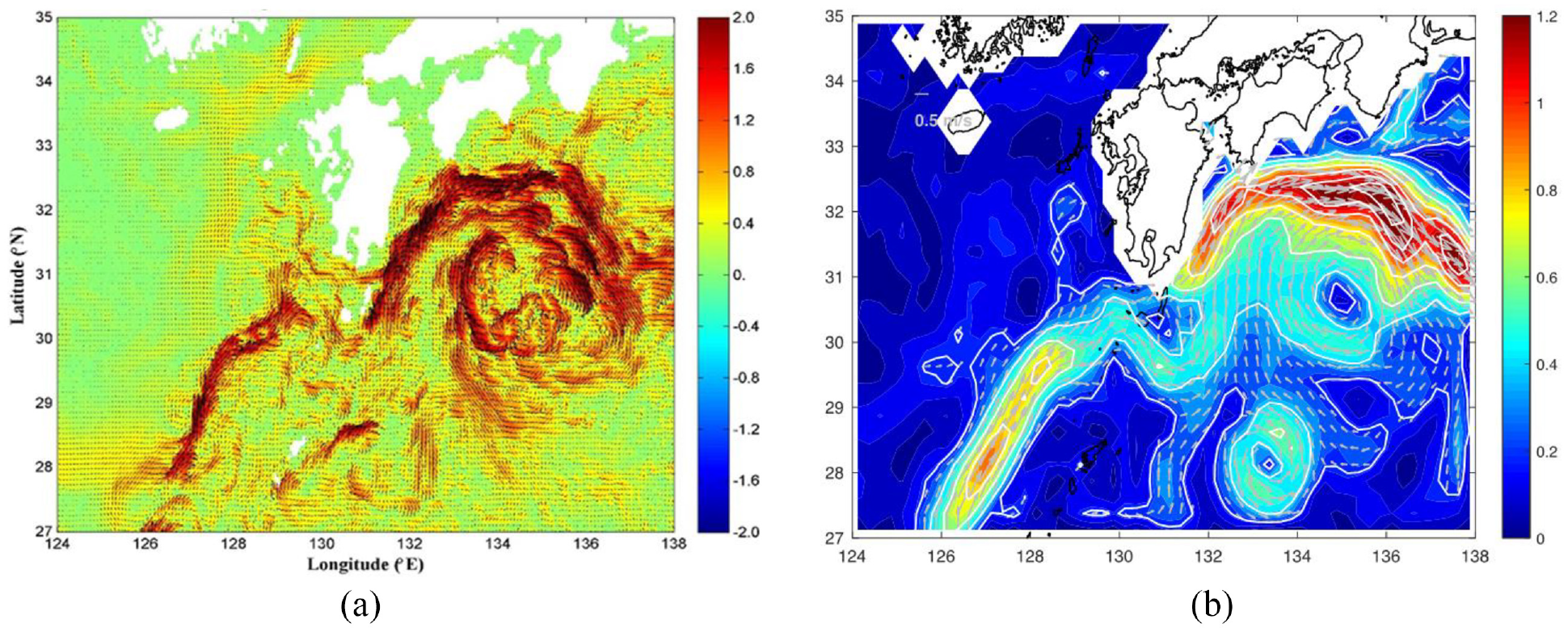
The configurations of ocean models.
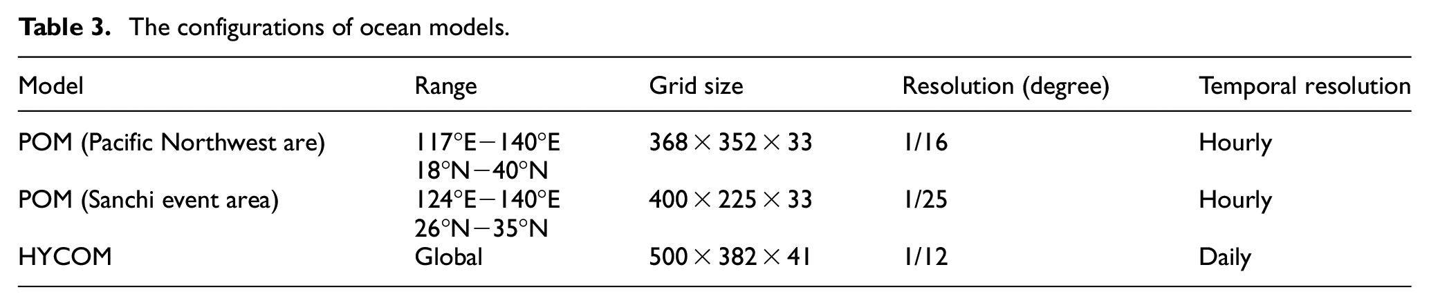
(a) Computational Kuroshio current from POM on 15 January, 2018 at 7:00. Color is the current speed and vectors are the surface current. (b) Sea surface height (color) and the geostrophic current (vector) and current speed (contour) from AVISO on 15 January, 2018. Dashed lines indicate the region for comparison between observation and model.
Short-term hindcast of oil spill
The movement of the oil slick on the surface after 24 and 144 h is shown in Figures 8 and 9, respectively. At 3 AM on 17 January, it can be seen from the present simulation that the oil was transported northeastward. This trend is in a good agreement with the current direction in Figure 7.
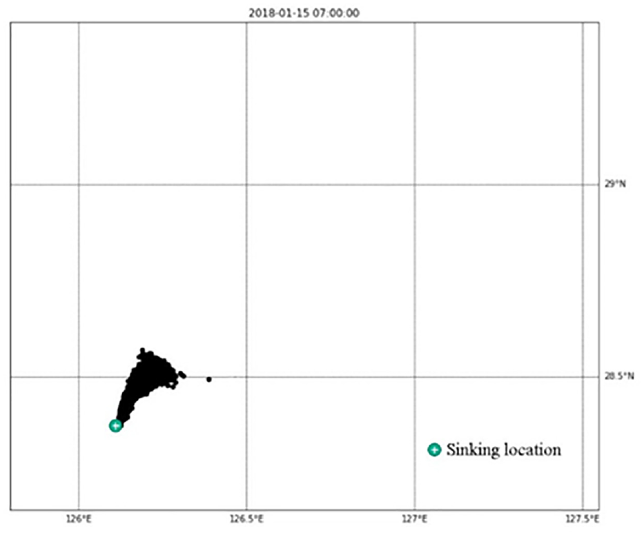
The oil slick at 07:00 on January 15 (24 h after oil spill).
The oil slick at 07:00 on January 20 (144 h after oil spill).
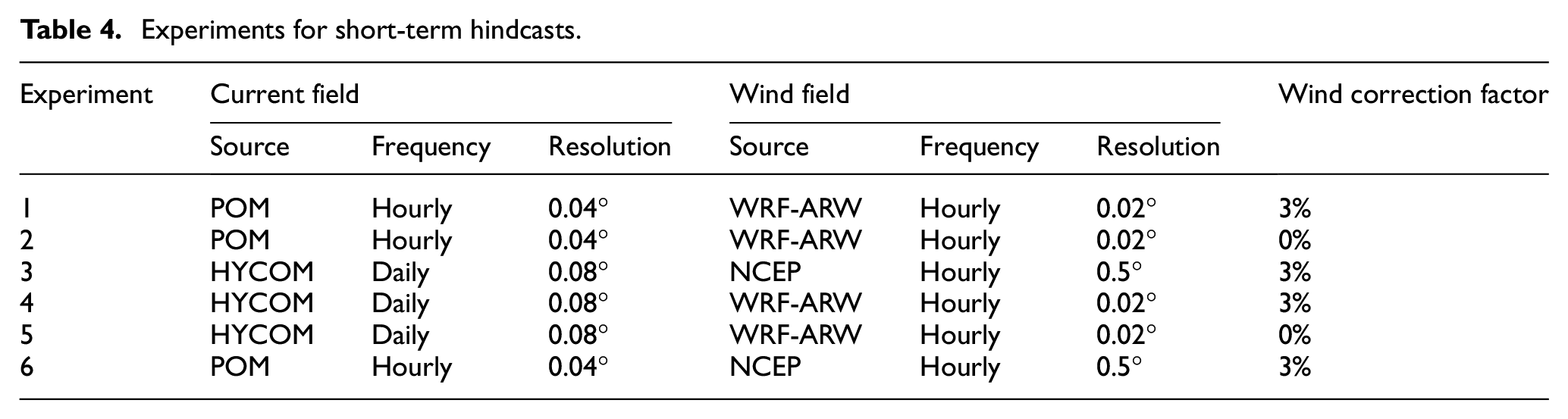
In order to study the forcing effects of wind and ocean data, several reference experiments (Experiment 2−Experiment 6) are conducted as compared with the default experiment 1 as addressed in Table 4. All of them have the same input parameters, as mentioned in Table 1. The experiments were designed to test the impact of water current from HYCOM and POM, and wind fields from the NCEP and WRF. The wind drift factor also was considered. While experiments 1, 3, 4, 6, the wind parameter was fixed at 3%, experiment 2 and 5, it was fixed at 0%.
Experiments for short-term hindcasts.
We make the comparison between them at two points of time: at 3 AM on January 17 (that has satellite image) and the end of the simulation period (7 AM on January 20). Figures 10 and 11 show the oil slick after 6 days of experiments 3, 4, 5, which use the current from HYCOM and of experiments 6, 1, 2, which use the current from POM. It can be seen that in both figures, image (a) and (b) with the different wind models are quite similar. Moreover, when we do not add the wind drift factor, the results change moderately (image (c)). Therefore, the wind effect driven by the wind drift factor is indispensable to the movement of oil particles.
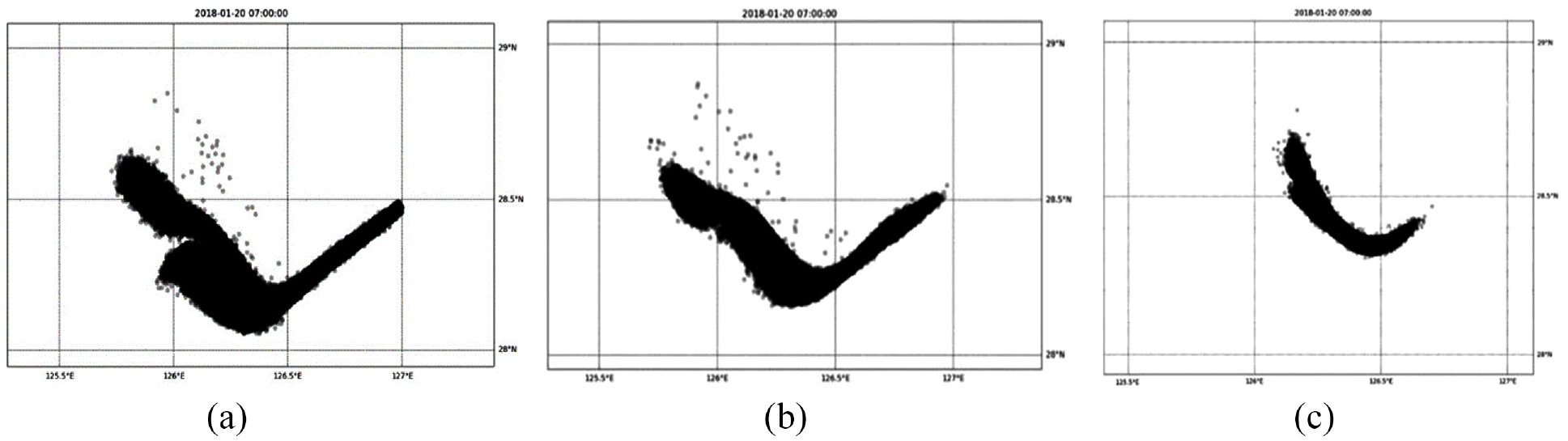
Position of the oil slick at 07:00 on January 20 in (a) Experiment 3, (b) 4, and (c) 5, which use the current from HYCOM.
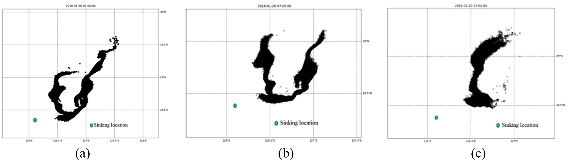
Position of the oil slick at 07:00 on January 20 in (a) Experiment 6, (b) 1, and (c) 2, which use the current from POM.
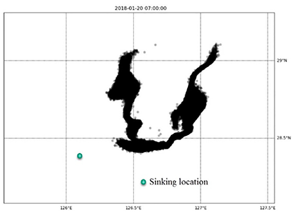
Sequentially, the simulated results at 3 AM on January 17 (Figure 12) are compared with the oil slick of the SPOT-6 satellite image (Figure 13) at 2:30 AM on January 17. In Figure 12, it can be observed that experiment 1 (POM & WRF-ARW with 3% wind) (a) and 6 (POM & NCEP with 3% wind) (b) have the results that the oil was transported northeastward, similar to the satellite image in Figure 13. However, the oil slick moved much further in the latter than in the former and in the image of satellite as well. While the all the results of experiment with HYCOM’s ocean current including experiment 3 (c), 4 (d), 5 (e) show the spilled oil particles move toward the northwest, experiment 2 (POM & WRF-ARW without wind drift factor) shows the northward movement and eastward displacement of the oil slick separately (f). This difference demonstrates the importance of the wind correction factor again. In addition, the simulated oil slick and that from the satellite image have similar dimensions of 56 km by 34 km and 54 km by 29 km, respectively.
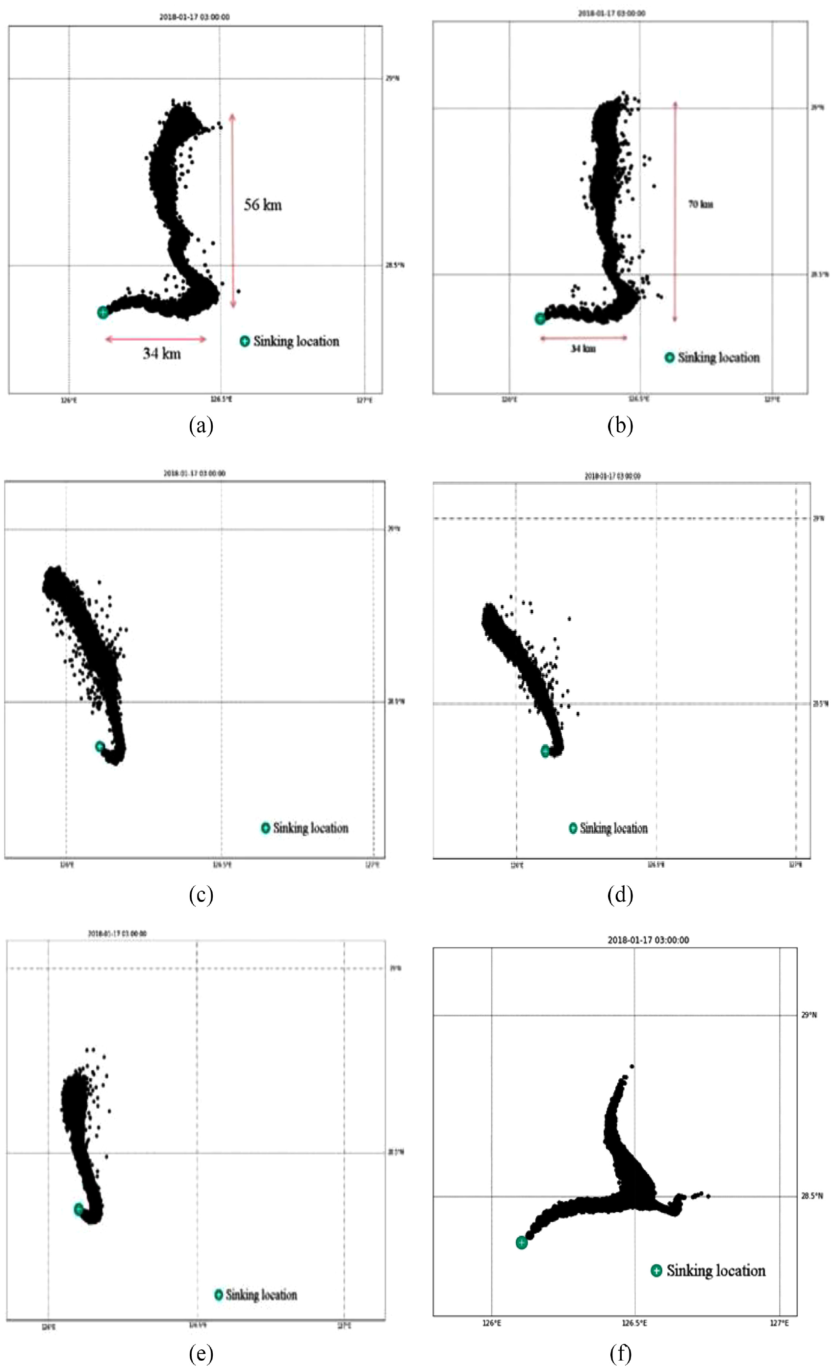
Position of the oil slick at 3 AM on January 17 in (a) Experiments 1, (b) 6, (c) 3, (d) 4, (e) 5, and (f) 2.
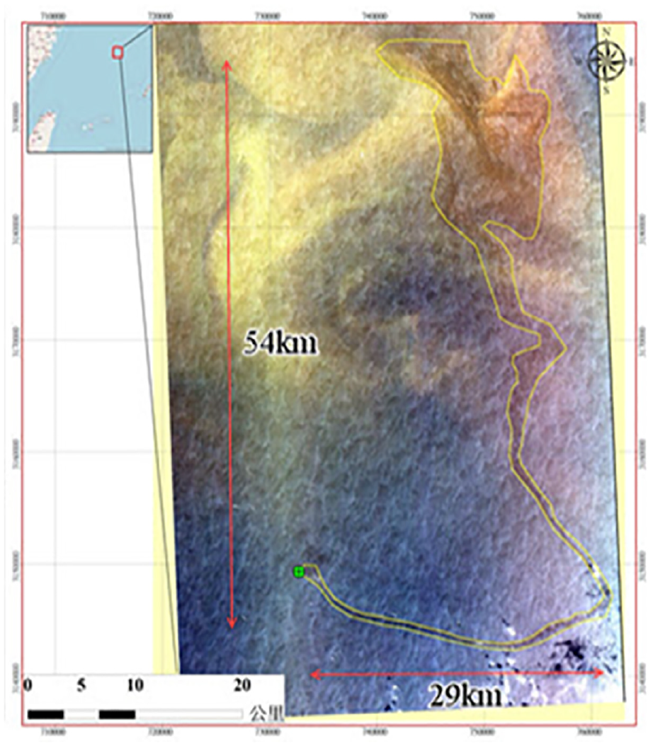
The oil slick of the SPOT-6 image at 2:30 AM on January 17.
Long-term hindcast of oil spill
In this part of the study, we use the integrated model, including POM, WRF-ARW, and OpenOil, to simulate the Sanchi oil spill in 1 month. It can be seen from the 30 days hindcast (Figure 14) that a large proportion of the oil particles move to the northeast of the sinking location. The majority of the particles would be trapped by Kuroshio. Apart from this, a small portion of spilled oil moves to the Japan Sea. The two routes are in coincidence with the significant spawning grounds and mitigation routes of some kinds of fish. After 1 month, about more than 15 islands in Southwestern Japan, which are known for the beautiful beach and extensive reef system, have effected. Oil pollution can have huge damage to the marine environment.
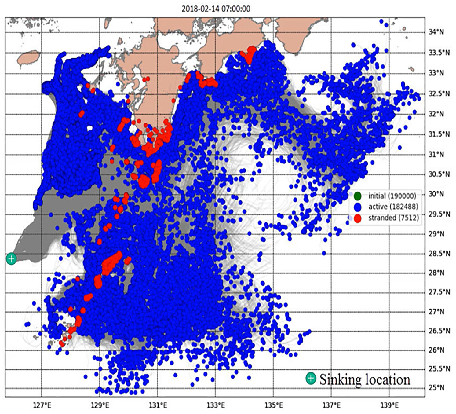
Position of the oil slick at 07:00 on February 14.
Conclusions
In this paper, an integrated model to predict the transport and fate of the oil spill is introduced. It is based on the Advanced Research Weather Research and Forecasting model (WRF-ARW) for meteorological forecast, the Princeton Ocean Model (POM) for hydrodynamic simulation in addition to OpenOil, a sub-module of OpenDrift, for oil spill model. This model was used to simulate the oil spill event involving the oil tanker Sanchi which occurred on the open sea in January 2018. After obtaining the wind field by developing a triple-nested simulation scheme for the high-resolution forecast and Kuroshio current in the East China Sea simulated by the POM, the Lagrangian particle-tracking model OpenOil was applied to simulate the oil spills. The proposed model is validated by the image of the SPOT-6 satellite, and a good agreement was obtained. Some reference experiments are designed for short-term hindcasts, and it is found that for the accuracy of the result, the high-frequency (hourly) and high-spatial-resolution models for input data is required and the wind correction factor has to be included. The 30day’s simulation for the Sanchi event demonstrates that the present model successfully applied for long-term prediction. These results have demonstrated that the present integrated model can be used to predict the fate and transport of oil spills with a huge amount of oil spilled in the open sea. In addition, the model can be applied more easily for other academic or operational utilizations as it is based on the open-source codes.
Footnotes
Declaration of conflicting interests
The author(s) declared no potential conflicts of interest with respect to the research, authorship, and/or publication of this article.
Funding
The author(s) disclosed receipt of the following financial support for the research, authorship, and/or publication of this article: This research was funded by the Ministry of Science and Technology of Taiwan under the Grant No. MOST 109-2221-E-019-061-MY3.
Data availability statement
Some or all data, models, or code that support the findings of this study are available from the corresponding author upon reasonable request.