Sage Journals: Discover world-class research

Abstract

This paper presents a deep learning method for the prediction of ship motions in 6 Degrees of Freedom (DoF). Big data streams of Automatic Identification System (AIS), now-cast, and bathymetry records are used to extract motion trajectories and idealise environmental conditions. A rapid Fluid-Structure Interaction (FSI) model is used to generate ship motions that account for the influence of surrounding water and ship-controlling devices. A transformer neural network that accounts for the influence of operational conditions on ship dynamics is validated by learning the data streams corresponding to ship voyages and hydro-meteorological conditions between two ports in the Gulf of Finland. Predictions for a ship turning circle and motion dynamics between these two ports show that the proposed method can capture the influence of operational conditions on seakeeping and manoeuvring.

Keywords

Ship motions big data fluid-structure interactions deep learning Gulf of Finland

Introduction

The use of accurate ship dynamics models is crucial for the development of intelligent decision support systems^1,2 and within the context of safe autonomous ship operations. Ship dynamics can be idealised by physics-based methods or by big data science.

Over the years, physics-based methods have been used to describe ship motion dynamics and their consequences based on classic ship theory. Examples include the Abkowitz³ and the Manoeuvring Modeling Group (MMG) models.⁴ Reduced order 4-DoF models or more detailed 6-DoF models have been developed to idealise the influence of nonlinear seakeeping and manoeuvring characteristics on ship directional control.^5,6 Kinematic models have also been introduced to better manage operational uncertainties and reduce computational costs. Recently, examples of rapid methods for the analysis of ship evasiveness during critical events have been proposed by, for example, Taimuri et al.,⁷ Gil et al.⁸ and Gil.⁹ In these methods, the hull-propeller-rudder interaction coefficients and hydrodynamic derivatives are used as critical parameters that represent original ship features. Common parameter determination tools include: the empirical method by Xu et al.,¹⁰ the captive model test method of Okuda et al.,¹¹ Computational Fluid Dynamics (CFD) modelling methods such as the one by Lu et al.,¹² as well as system identification approaches, for example, Ramirez et al.¹³ Their application is extremely useful for ship manoeuvring simulations at the ship design stage. However, they fail to present a unified and convincing prediction of ship motions under environmental conditions in real-time.

Research in big data science may help overcome problems associated with identifying coefficients and hydrodynamic derivatives in real-time via the utilisation of model tests or open sea-trial data. Parametric estimation methods are used to quantify ship dynamics, given that available ship mathematical models are in place to train big data streams. For example, Wang et al.¹⁴ applied the nu-support vector machine to identify the hydrodynamic derivatives of the 3-DoF Abkowtiz model. Zeng et al.¹⁵ used the Extended Kalman Filter (EKF) method to determine the hydrodynamic derivatives of an MMG model. Non-parametric estimation models use Artificial Neural Networks (ANN), Long Short-Term Memory (LSTM), Gaussian process regression and locally weighted learning methods to predict ship motion dynamics based on the simulated free-running tests. For example, Silva et al.,¹⁶ Ouyang et al.,¹⁷ Ramirez et al.,¹³ Woo et al.,¹⁸ Sivaraj et al.¹⁹ Notably, Lou et al.²⁰ developed neural network models for the prediction of motions of unmanned surface vehicles using results from open seas manoeuvrability tests in 3-DoF. Notwithstanding this, most parametric or non-parametric statistical regression models ignore the influence of medium to long-term environmental conditions or seabed topology (shallow waters/deep waters).

The idealisation of environmental conditions is possible via the use of big data science. Ship motion trajectory prediction methods that utilise big data streams (e.g. AIS data, new-cast data) are classified as statistical, machine learning and deep learning methods. Examples of statistical methods are the single point neighbour search,²¹ the k-order Markov chain²² and the particle filter²³ methods. Machine learning methods involve Gaussian process regression models,²⁴ support vector machines,²⁵ and k-nearest neighbours.²⁶ Finally, examples of deep learning methods are convolutional neural networks,²⁷ LSTM,²⁸ bidirectional Gated Recurrent Units (GRU)²⁹ and transformer^30,31 algorithms. The latter can train historical AIS data to capture limited ship motion features and predict ship motion trajectories in advance.³² However, their use is motivated by traffic management theory. They ignore environmental conditions and do not account for the influence of the sea loads on ship dynamics. Recently, Zhang et al.² proposed a Gaussian process regression method, which can be used to predict time-varying ship motion trajectories in real operational conditions. However, since AIS data only includes a little dynamic information regarding ship motion trajectory, prediction methods underestimate ship control devices (ruder and thruster) and ignore some of the ship motion features (i.e. roll, pitch, yaw, etc.).

This paper pushes forward state-of-the-art by introducing a deep learning method for the prediction of 6-DoF ship motions in real conditions. The method uses AIS data records and bathymetry data to extract ship motion features in real conditions (See Ship motion features extraction). The ship dynamics model of Taimuri et al.³³ is used to generate ship motions in 6-DoF. The model accounts for the influence of control devices (see 6-DoF FSI ship grounding dynamics model). Consequently, a deep learning model is developed to learn AIS data streams corresponding to real operational conditions between two ports (Tallin and Helsinki) in the Gulf of Finland. The trained model predicts 6-DoF ship motions in real conditions and turning circles in calm waters. The practical application of the approach is demonstrated by using data covering a 13-month ice-free period for a Ro-Pax Passenger ship (see Case studies). The paper concludes with some ideas on the potential use of the method to develop automatic ship control systems (see Conclusions).

Methods

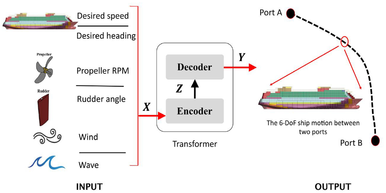
The deep learning method used for the prediction of 6-DoF ship motion dynamics accounts for ship theory, rigid body dynamics, historical motion features and the influence of environmental conditions (wind, wave, and water depth). The methodology comprises the following three steps (see Figure 1):

Step I: Ship motion features extraction. Here AIS ship trajectories are reconstructed for the case of a ship operating between two ports. Time-domain hydro-meteorological data are extracted from now-cast data providers. GEBCO bathymetry data are used to construct the waterway. Data streams are then integrated to extract ship motion features and environmental conditions.

Step II: Ship grounding dynamics model development. Data from Step-I are used as input in an FSI model³³ to idealise the influence of operational conditions and controlling devices. As part of this process, the Proportional Derivative (PD) controller is used to control the rudder based on the predefined heading of the ship that resulted from Step-I. This autonomously steers the ship on the desired AIS track of each voyage in real time.

Step III: Deep learning model development. A transformer model is constructed for the prediction of long-term ship motion dynamics. Results of 500 voyages obtained from Steps I and II are based on training a 6-DoF transformer model using 80% of the available big data streams between two ports. Model validation and model testing are based on the remaining 20% of the total data set corresponding to the same route and ship.

Notably, if actual ship operation data is given for training a transformer based 6 DOF ship motion predictor, the ship dynamics model in Step II should be excluded from the entire framework and should be replaced with actual ship operation data from sea trials.

Figure 1.

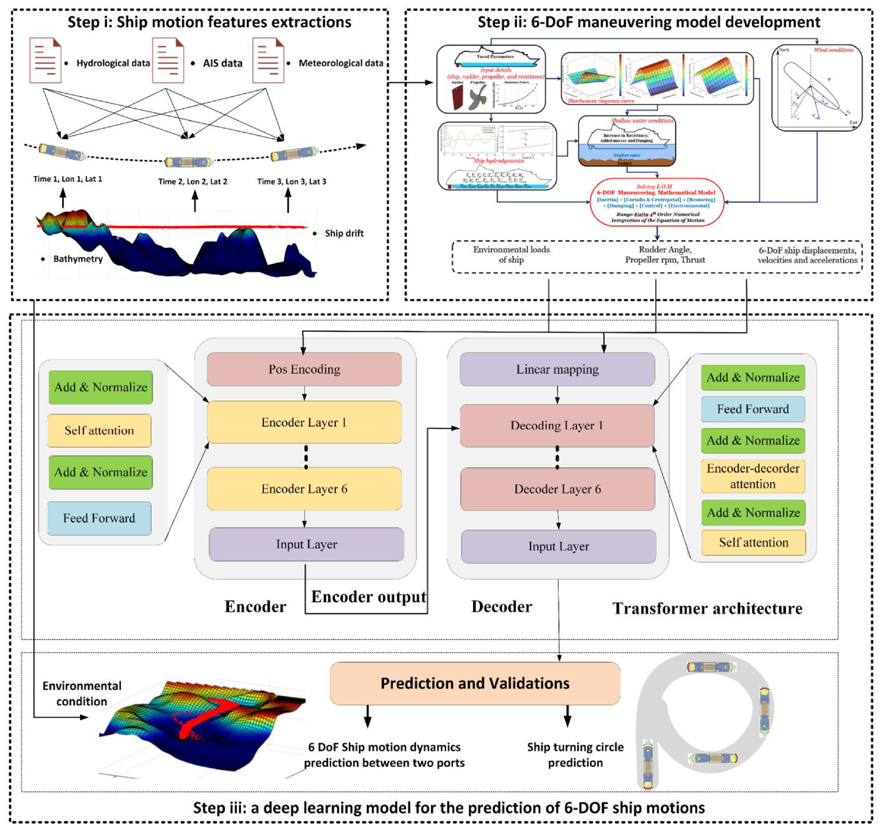
The transformer framework for the prediction of 6-DoF ship motion.

Ship motion features extraction

To extract ship motion features (the heading, trajectory, and speed) and real environmental conditions (weather conditions and waterways conditions), AIS, hydro-meteorological data records, and bathymetry data made openly available,¹ are used, see Figure 2. The specifics are explained by Zhang et al.³⁴ AIS data contain static data streams (e.g. ship size, voyage, ship type, etc.) and dynamic data streams (e.g. speed, course, heading, etc.). Those are reconstructed to remove outliers. The process aims to avoid erroneous streams related to data collection, transmission, and reception.^35,36 Ocean now-cast records may replace the weather data measured onboard ships. This is because the now-cast data agrees with real weather data collected on weather buoys.³⁷ AIS and now-cast data are mapped on the bathymetric map to extract waterway conditions.

Figure 2.

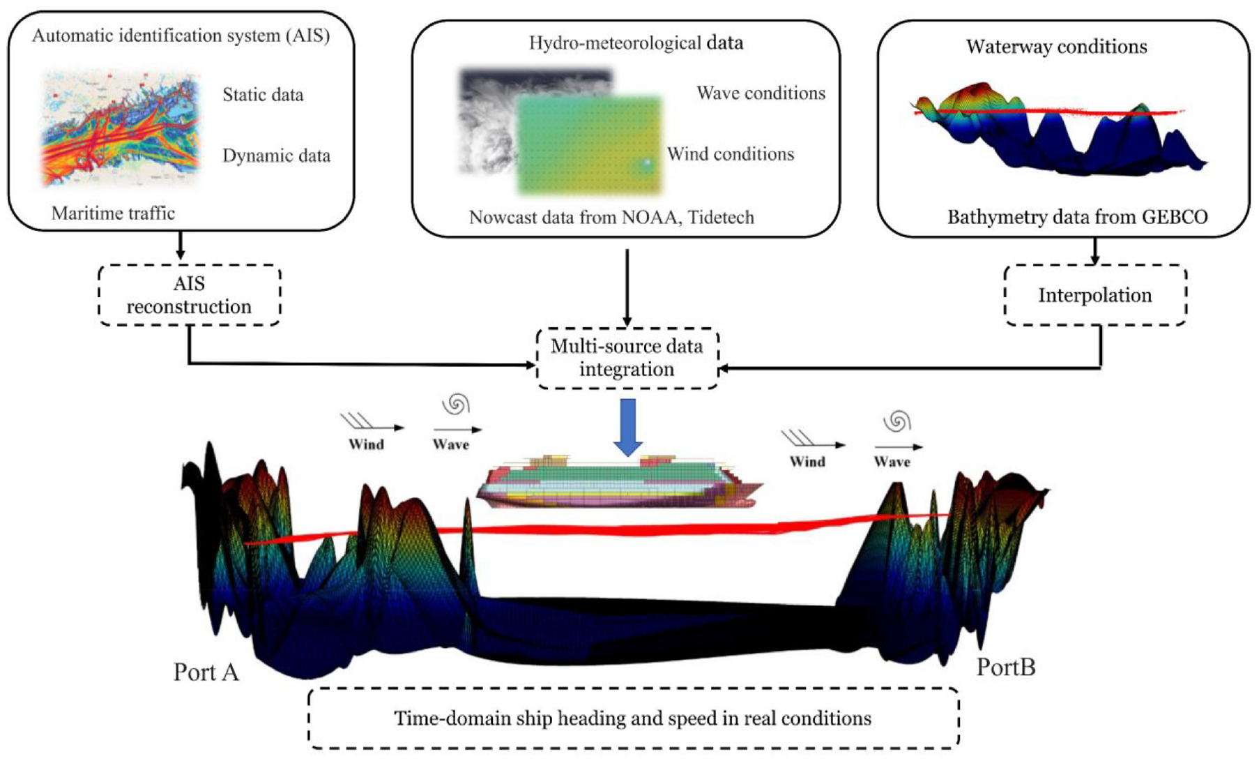
Ship motion features extraction from big data streams.

Since AIS and now-cast data may not be transmitted or updated at the same time, data streams of different sources may appear to be out of sync. The time intervals and resolutions of AIS, now-cast data, and bathymetry data can be different in the temporal-spatial domain. To integrate different sources of data, a multi-source data fusion model can be used.³⁸ Consequently, the operational condition and ship motion features (desired speed and heading features) between two ports can be extracted (see Figure 2).

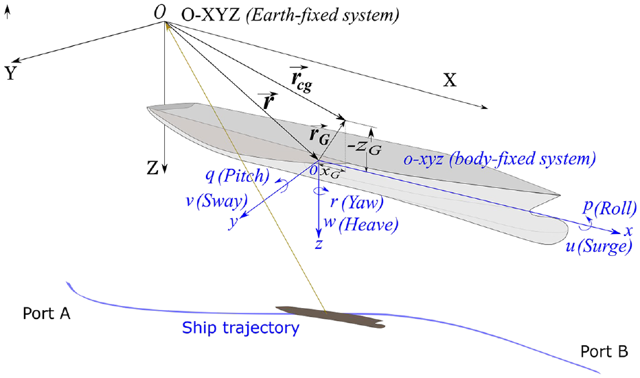
To capture the impacts of hydro-meteorological conditions on ship motion dynamics using the deep learning model, the wind angle and wave angle are transferred to the ship-based coordinate system depicted in Figure 3.

Figure 3.

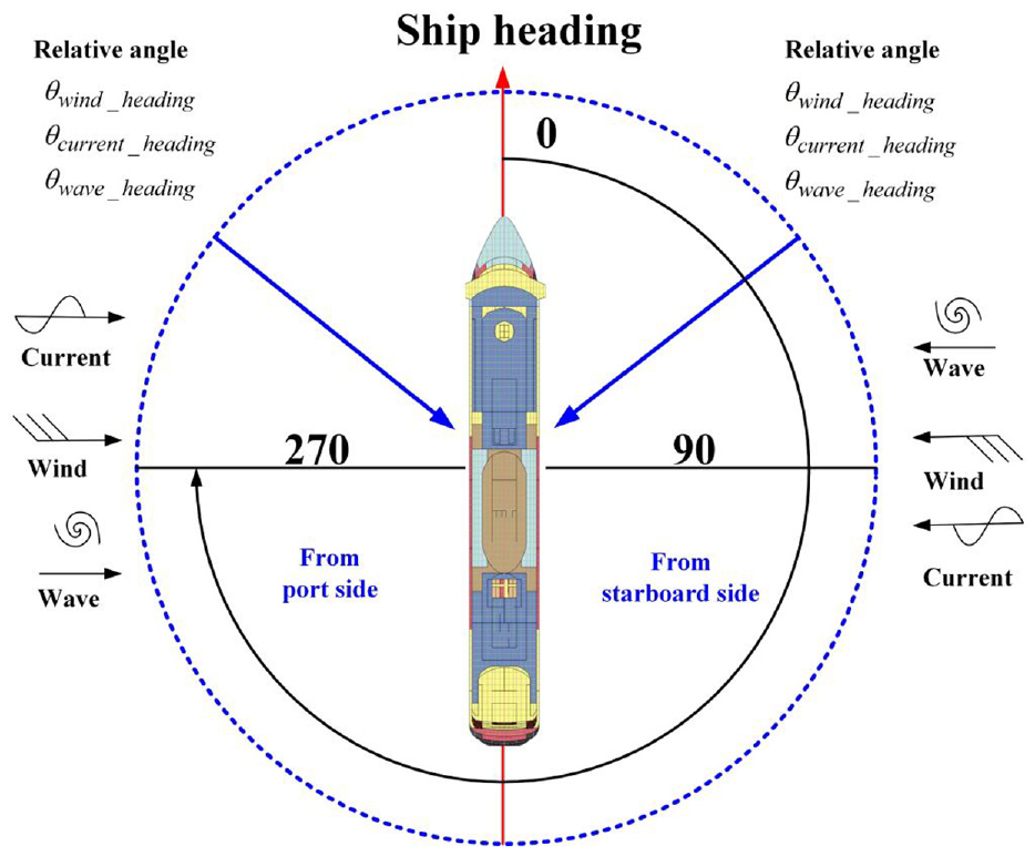
Relative directions between wave/ wind and ship heading.

6-DoF FSI ship grounding dynamics model

Operational data streams (i.e. available time series) are usually limited and only include information on ship speed, course and heading. Since wind and wave statistics come from different sources, there are uncertainties associated with the data collected from dedicated sea trials. Collection of data streams 6-DoF ship motions, rudder angles, propeller revolutions over the long term and across fleet databases is not practical. The same holds for data relevant to the forces acting on a ship (e.g. wind, waves, shallow water) the collection of which requires a large amount of measuring equipment. To overcome these challenges Physics based models can be utilised.

In this paper, results from the ship dynamics model of Taimuri et al.³³ are implemented in a deep learning method. The aim is to predict ship motions in 6-DoF by using input conditions corresponding to realistic rudder angles, ship speeds and environmental conditions. AIS data streams provide the motion features of the ship (heading, trajectory, and speed). Physics-based models are used to account for the influence of environmental conditions and ship dynamics. Wind data contain speed and angle with respect to the earth-fixed system. Short wave data include wave height, period and angle. Under severe circumstances, aerodynamics can affect ship dynamics. The loads due to wind on a passenger ship can be estimated based on the Blendermann method.³⁹ The 6-DoF ship dynamics model accounts for shallow water effects, and shortwave forces as explained in Taimuri et al.⁷ Figure 4 summarises the method used.

Figure 4.

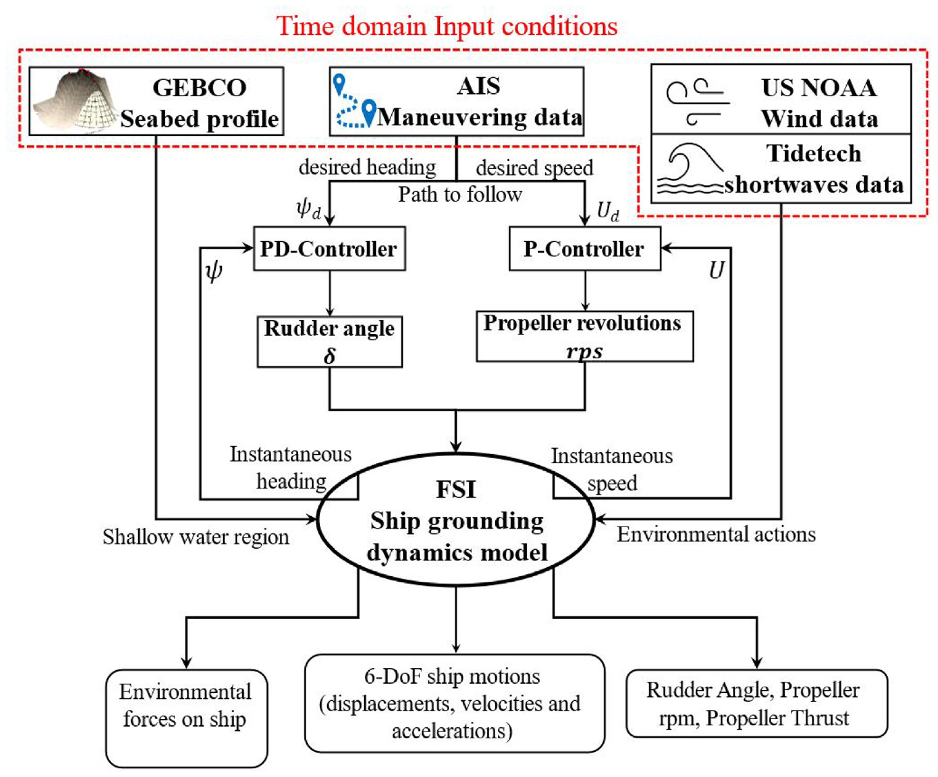
6-DoF FSI ship grounding dynamics model. Representing ship path following using the input from AIS, GEBCO and now-cast data.

Depending on the input parameters (see Figure 4), the path provided by the AIS data is followed using the autopilot control system. Rudder action is used to control the ship course based on the desired heading which has been set through AIS data. A simple Proportional Derivative (PD) controller is defined to set the target rudder angle ( $δ_{T}$ ) maintaining ship heading $ψ_{d}$ ⁴⁰ as:

δ_{T} = K_{p} (ψ - ψ_{d}) + K_{D} \overset{\cdot}{ψ}

(1)

where $K_{P}$ and $K_{D}$ are the gain factors of autopilot. The linear differential equation used to assess the rudder angle set by the autopilot controller is

\overset{\cdot}{δ} = sgn (δ - δ_{T}) ω_{δ}

(2)

In equation (2) $ω_{δ}$ is the rate of turn of the rudder. To obtain the desired speed $(U_{d}$ ) a P-controller is used, to control the revolution of the ship propeller. Initially, the revolution of the propeller is set according to the instantaneous ship speed ( $U$ ) as proposed in Taimuri et al.⁷ The value depends on the desired speed $(U_{d}$ ) from AIS data.

The new propeller rotation rate $N_{rp s_{new}}$ is defined as:

N_{rp s_{new}} = \frac{- k_{T 1} V_{A} ρ D^{3} + \sqrt{{(k_{T 1} V_{A} ρ D^{3})}^{2} + 4 k_{T 0} ρ D^{4} (V_{A}^{2} ρ D^{2} k_{T 2} - X_{Pro p_{new}})}}{2 k_{T 0} ρ D^{4}}

(3)

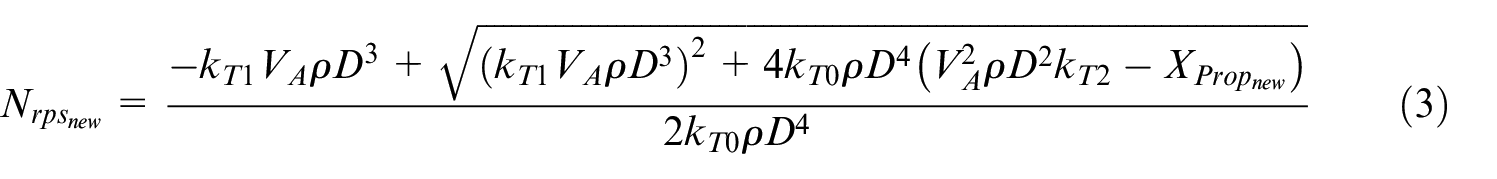
where $k_{T 0}, k_{T 1}, and k_{T 2}$ are second-order polynomial coefficients of propeller thrust characteristics curve having the propeller diameter of D. $X_{Pro p_{new}}$ is the desired propeller thrust at the ship advanced speed of $V_{A}$ ( $V_{A} = (1 - w) U_{d}$ ).

The new propeller revolution per second $N_{rp s_{i}}$ (RPS) is defined as:

N_{rp s_{i}} = K_{p_{rev}} (U_{d} - U) + N_{rp s_{new}}

(4)

where, $K_{p_{rev}}$ is the propositional gain of the P-controller. Consequently, the ship control devices (rudder angle, propeller rpm), and ship motion dynamics under the influence of environmental conditions are generated in real conditions.

Ship motion dynamics estimation transformer

Deep learning is a branch of Artificial Intelligence (AI) that imitates knowledge creation. Deep learning algorithms are stacked in a hierarchy of complexity and abstraction. The fundamental nature of the deep learning model is idealised by ANN (Artificial Neural Networks).^41,42 The transformer is an advanced architecture of deep learning that employs the mechanisms of self- and multi-head attention.⁴³ It can handle differentially weighting technology to determine the significance of features of input data often used in Natural Language Processing (NLP) and computer vision.^44,45

In this section, we propose a transformer-based deep learning method. The model is trained to predict ship motions in real conditions by historical voyage data between two ports. Figure 5 presents voyage data voyage data containing time series of ship motions (interval 1 s) under the influence of environmental conditions for the case of a voyage from port A to B (see 6-DoF FSI ship grounding dynamics model). For each point on the trajectory, the ship control actions, desired inputs, environmental conditions and 6-DoF ship motions are included. In this paper, 400 ship trajectories are combined as training data sets and 100 ship trajectories are selected for validation and testing (see Figure 6).

Figure 5.

6-DoF ship motion dynamics along ship trajectory between ports.

Figure 6.

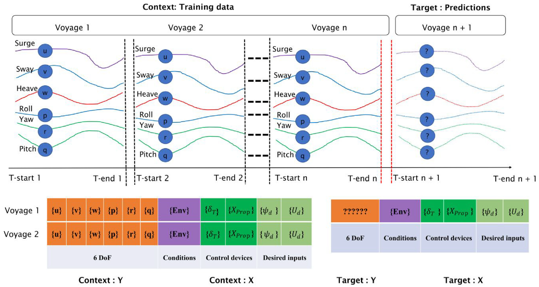
6-DoF ship motion dynamics predicting from autoregression theory perspectives (The lines denote the ship motion time series between two ports; the context data {X, Y} denote the historical data; the Target {Y} represents the predicted results in the future based on the Target {X}).

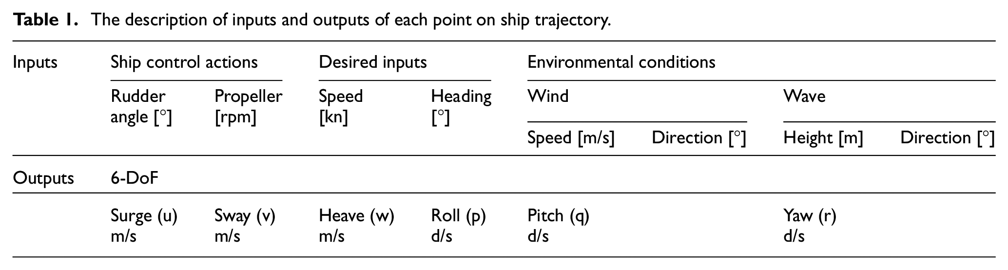
The trained model can be used to predict ship motions in real conditions as well as to predict ship turning circles in calm waters. The training data contain (a) context {X} that idealises environmental conditions, desired inputs (heading angle and speed), ship control actions (rudder angle, propeller rpm), and (b) context {Y} that idealises 6-DoF ship motion dynamics (Surge-u, Sway-v, Heave- w, Roll-p, Pitch-q, and Yaw-r) of each voyage (see Figures 5 and 6). The inputs of the trained model are target {X}, including environmental conditions, control devices, and desired inputs. The output is denoted by target {Y} containing 6-DoF ship motions, see Figure 6. More detailed explanation of the input and output vectors of a point on a ship voyage is presented in Table 1.

Table 1.

The description of inputs and outputs of each point on ship trajectory.

Inputs	Ship control actions		Desired inputs		Environmental conditions
	Rudder angle [°]	Propeller [rpm]	Speed [kn]	Heading [°]	Wind		Wave
					Speed [m/s]	Direction [°]	Height [m]	Direction [°]
Outputs	6-DoF
	Surge (u)	Sway (v)	Heave (w)	Roll (p)	Pitch (q)		Yaw (r)
	m/s	m/s	m/s	d/s	d/s		d/s

A transformer-based deep learning method is adopted to train big data streams and predict long-term ship motion time series in advance. The trained model can identify ship systems and predict 6-DoF ship motions between two ports (see Figure 7). The method accounts for the attention mechanism and the feed-forward neural network in the decoder and encoder modules. Regarding the attention mechanism, the more detailed description is presented by Vaswani et al.⁴³ The model is a sequence-to-sequence model, mapping sequences to the neural network for training data and predicting dynamics.⁴⁶

Figure 7.

Transformer architecture for ship motion time series prediction.

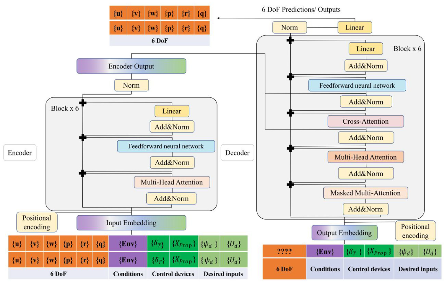
The architecture of the transformer is shown in Figure 8. It contains encoder and decoder modules. The encoder and decoder modules include many blocks (see representative blocks of the encoder and decoder in the grey areas in Figure 8). The mechanism is different to traditional neural networks. Transformer models present their architecture based on blocks instead of neurons.⁴⁶ In the paper, both the encoder and decoder modules have six blocks. The block in the encoder has four layers, and the block in the decoder has six layers. Their functions can be described as follows:

The encoder includes multi-head attention and a feedforward neural network. The purpose of the encoder module is to map the time series of operational conditions, control devices, and desired inputs (see $matrix X$ in equation (5)) to a new continuous series (see $matrix Z$ ) in Equation (6)). The process is carried out based on the “attention mechanism”, which is presented as function $softmax$ in equation (10).

The decoder module contains masked multi-head attention, multi-head attention, cross-attention, and a feedforward neural network (see Figure 8). It aims to generate and / or predict the time series of ship motions (see matrix Z in equation (7)) based on an autoregressive method.⁴³ Because of the use of the attention mechanism in the deep learning model, it is less likely to forget information from the big data streams of training and predicting.⁴⁶

X = {x_{1}, x_{2}, x_{3}, \cdot \cdot \cdot, x_{n}}

(5)

Z = {z_{1}, z_{2}, z_{3}, \cdot \cdot \cdot, z_{n}}

(6)

Y = {y_{1}, y_{2}, y_{3}, \cdot \cdot \cdot, y_{n}}

(7)

In the above equations, $X$ denotes the matrix of control devices, conditions, and desired inputs in the time domain; $Y$ denotes the matrix of the 6-DoF ship motion in the time domain; $Z$ denotes a matrix. $x_{n}$ denotes the inputs of control devices, conditions, and desired inputs at point $n$ . $y_{n}$ denotes the outputs of 6-DoF at point $n$ .

Figure 8.

Transformer architecture for 6-DoF ship motion prediction.

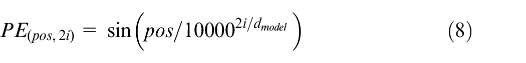
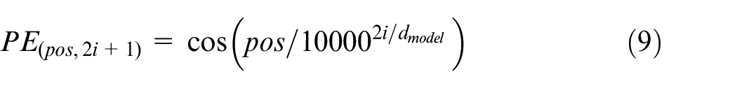
This deep learning network includes encoder and decoder stacks of multiple layers of attention (see Figure 8). Next, the process and each part of the deep learning model are described. First, the inputs (time domain ship motion of each voyage, see Figures 5 and 6 will be transferred to the Input Embedding layer. The time domain ship motion of each voyage can be regarded as a lookup table to capture a learned vector representation of the ship motion of the voyage. The feed – forward neural network layer learns the number of lookup tables from the training database. In this way, the ship motions data streams from each voyage can be clustered in the form of vectors. The smart positional encoding scheme is used to inject the location information into the vector from the Input Embedding layer. This is because the sea depth of the waterway varies along the voyage and influences ship motions. The calculation processes of positional encoding are defined in equations (8)–(9). This is a common way to define the position of inputs and outputs.⁴⁶ Embedding and positional encoding of inputs (i.e. the idealisation of ship motions corresponding to each voyage in the time domain) are combined as input vectors to the encoder and decoder modules. These data are used to train the model.

P E_{(pos, 2 i)} = \sin (pos / 10000^{2 i / d_{model}})

(8)

P E_{(pos, 2 i + 1)} = \cos (pos / 10000^{2 i / d_{model}})

(9)

In the above equations $pos$ denotes the location of the time series of ship motions, and $i$ presents the dimensionality of $d_{model}$ .

Once the vector with the positional encoding is transferred to the encoder and decoder module (see Figure 7), the encoder module is used to map the time series of inputs to a new continuous series. The decoder module is used to generate the output time series of ship motions prediction based on auto-regressive technique (see equations (5)–(7)). The encoder and decoder have similar sub-layers.

The encoder and decoder modules include (1) Attention mechanism/multi-head attention/marked multi-head attention layer; (2) Add and Norm function layer; (3) Feed-forward networks (FFN) layer; (4) Linear layer, see in Figure 8. The mechanism and purposes are explained below:

Attention mechanism/multi-head attention layer

The attention mechanism enables the deep learning model to have extremely long-term memory for ship motion time series. Hence the model can attend to or focus on all the ship motion information throughout the voyage. The attention layer and $softmax$ functions are defined according to equation (10) in the transformer architecture, see more in Vaswani et al.⁴³

z = Attention (Q, K, V) = softmax (\frac{Q K^{T}}{\sqrt{d_{k}}}) V

(10)

In equation (10), $Q$ , $K$ and $V$ are query, key and information value vectors, $Q \in R^{n \times d_{k}}, K \in R^{m \times d_{k}}, V \in R^{m \times d_{v}}$ are the matrixes, including query, key, and value of attention; $d_{k}$ denotes the dimensions in blocks. In addition, based on equations (5) and (6), $Q = X \times QW$ , $K = X \times KW$ , $V = X \times VW$ . $QW, KW, and VW$ are weight matrix. 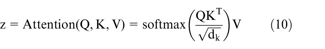$z$ denote an element of the matrix $Z$ which is calculated using $softmax$ functions by equation (10).

Each attention process is regarded as a head to learn ship motions. For each head, an output vector can be predicted and multi vectors can be concatenated into a single output vector. Therefore, a multi-head attention can learn more information about ship motions than a single attention layer. The multi-head attention layer contains attention layers. The multi-head attention layer is defined as shown in equations (11) and (12). The marked multi-head attention is a hidden multi-head attention layer. The mask denotes a matrix to the scaled attention scores of the multi-head attention layer, see more in Bhattacharya et al.⁴⁷

MultiHead (Q, K, V) = Concat ({head}_{1}, \dots, hea d_{h}) W^{O}

(11)

In equation (11), $W^{o} \in R^{h \times d_{model} \times d_{k}}$ , $h$ denotes the number parallel attention layers.

hea d_{i} = Attention ({QW}_{i}^{Q}, {KW}_{i}^{K}, {VW}_{i}^{V})

(12)

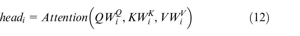
In equation (12), $QW, KW, and VW$ are weight matrix, $W_{i}^{Q} \in R^{d_{model} \times d_{k}}$ , $W_{i}^{k} \in R^{d_{model} \times d_{k}}$ , $W_{i}^{v} \in R^{d_{model} \times d_{k}}$ .

Add and Norm layers

To add the outputs vector from the hidden multi-head attention layer to the original positional input embedding of time domain ship motion, Add & Norm layers are needed. The Add layer contains a residual network or residual connection. Its aim is to learn the residual functions of inputs, as given in equation (13). The output of the Add goes through a Norm layer. The Norm is a layer normalisation used to improve the performance and training time as given in equations (14)–(16).

F (x) = H (x) - x

(13)

μ^{l} = \frac{1}{h} \sum_{i = 1}^{h} a_{i}^{l}

(14)

σ^{l} = \sqrt{\frac{1}{h} \sum_{i = 1}^{h} {(a_{i}^{l} - σ_{μ}^{l})}^{2}}

(15)

\hat{a^{l}} = \frac{a^{l} - σ_{μ}^{l}}{\sqrt{{(σ^{l})}^{2} + ε}}

(16)

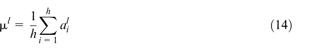
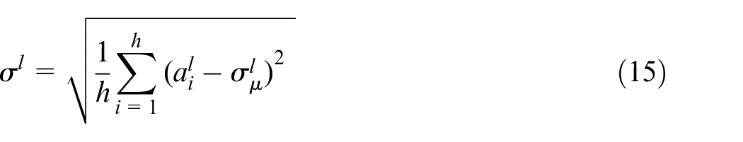
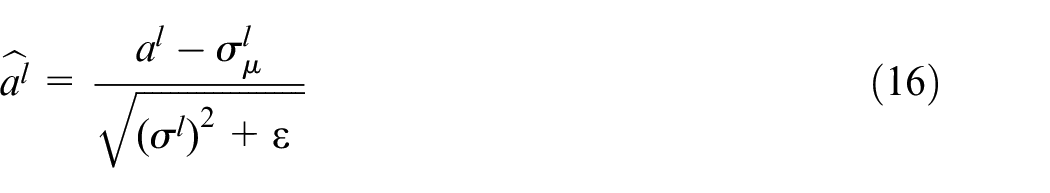
In the above equations $H (x)$ is the desired mapping, $F (x)$ denotes the stacked nonlinear layers, and the original mapping reconstructed as $F (x) + x$ ; $h$ denotes the number of nodes of the hidden layer; $l$ denotes the number of layers. The $σ^{l}$ and $μ^{l}$ are the parameters of layer normalisation; $σ_{μ}^{l}$ is the mean value; $\hat{a^{l}}$ denotes the results of layer normalisation and $ε$ denotes a very small number that can be used to avoid $\sqrt{{(σ^{l})}^{2} + ε}$ = 0 (see equation (16)).

Feed-forward network

The output of Add & Norm gets projected through feed-forward networks for further processing. The Feed-Forward Network (FFN) is used to stabilise the network and reduce the training time. The FFN comprises of a couple of linear layers. Between the linear layers, a ReLU (Rectified Linear Units) activation is used to connect each sub-layer, see more in Li et al.⁴⁸ The concept is defined as follows:

FFN (x) = max (0, x W_{1} + b_{1}) W_{2} + b_{2}

(17)

ReLU (x) = (x)^{+} = max (0, x) = {\begin{matrix} \begin{matrix} x & if x > 0 \end{matrix} \\ \begin{matrix} 0 & if x \leq 0 \end{matrix} \end{matrix}

(18)

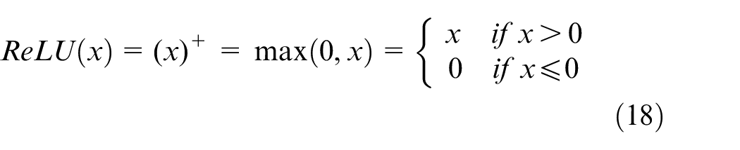
In equation (17), the function max () denotes the ReLU function as per equation (18); $W_{1}$ , and $W_{2}$ represent the value of slope; $b_{1}$ , and $b_{2}$ represent the value of intercept.

Linear layer

The decoder is capped off with a linear layer that acts as a classifier to present the predicted outputs. The linear function is a linear transformation of data streams,⁴³ defined as :

y = x A^{T} + b

(19)

where, $A^{T}$ represents the value of slope; $b$ represents the value of intercept.

To capture more ship motion features from historical ship motion dynamics in real conditions, the encoder and decoder are defined as a stack of six blocks. This is because the proposed model includes six blocks in the encoder module and six blocks in the decoder module. To save training time, the outputs of the dimension $d_{model}$ are set as 256. So, the proposed model employs one parallel attention layer in a block of the encoder module and three parallel attention layers in a block of the decoder module. Each of the inner layers includes 1024 dimensions. The complex architecture of the transformer gives the opportunity to learn different ship motion dynamics in real conditions, potentially boosting the predictive ability of the ship manoeuvring features of the selected ship.

To calculate the errors between the real and the predicted ship motion dynamics, Root Mean Square Error (RMSE), Mean Absolute Error (MAE), and $R^{2}$ (Coefficient of Determination) are used as follows:

RMSE = \sqrt{\frac{1}{N} \sum_{n = 1}^{N} {(y_{n} - \overset{\land}{y_{n}})}^{2}}

(20)

MAE = \frac{\sum_{n = 1}^{N} | y_{n} - \overset{\land}{y_{n}} |}{N} = \frac{\sum_{n = 1}^{N} | e_{n} |}{N}

(21)

R^{2} = 1 - \frac{\sum_{n = 1}^{N} {(y_{n} - \overset{\land}{y_{n}})}^{2}}{\sum_{n = 1}^{N} {(y_{n} - \bar{y_{n}})}^{2}}

(22)

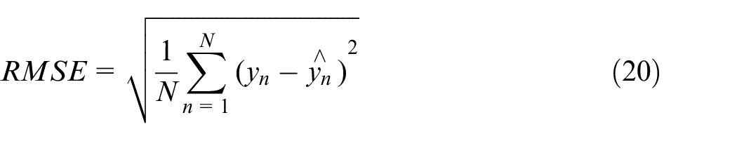
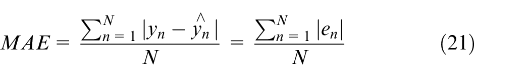
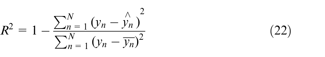
In the above equations $y_{n}$ is the actual value, $\overset{\land}{y_{n}}$ denotes the predicted value and $\bar{y_{n}}$ is the mean value while $| e_{n} |$ represents the absolute errors.

Case studies

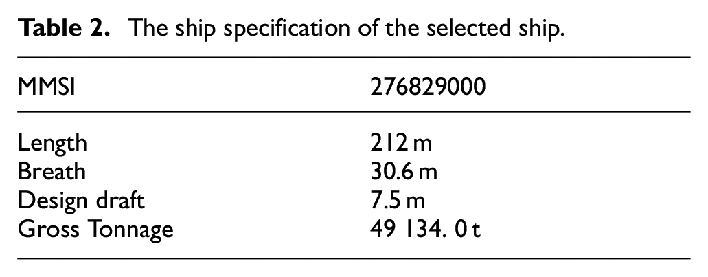
To validate the proposed method, a typical Ro-Pax ship cruising between Helsinki and Tallinn was selected (see Table 2). The data sample corresponded to 500 voyages that took place over the ice-free period between 2018 and 2019. It is noted that the waterway between Helsinki and Tallinn may be frozen in the winter period (December, January, and February). However, this is not considered here. For model training, validation, and testing, the 500 voyages of the ship from Helsinki to Tallinn were classified into three data sets namely : (1) training data set - 400 voyages (80%); (2) validation data set – 50 voyages (10%); (3) testing data set – 50 voyages (10%). To better understand the generalisation ability of the trained model, the turning circles of the ship were predicted based on the new inputs. The rudder angles were set as 1°, 5°, 10° and 15°, starboard; while propeller revolutions were kept constant at 109 rpm.

Table 2.

The ship specification of the selected ship.

MMSI	276829000
Length	212 m
Breath	30.6 m
Design draft	7.5 m
Gross Tonnage	49 134. 0 t

Extracting ship motion features in real conditions

Ship trajectories of the selected ship were extracted from the AIS database and clustered to identify the ship voyages from Helsinki to Tallinn, see more in Zhang et al.³⁸ GEBCO data were used to generate the sea floor, see Figure 9.

Figure 9.

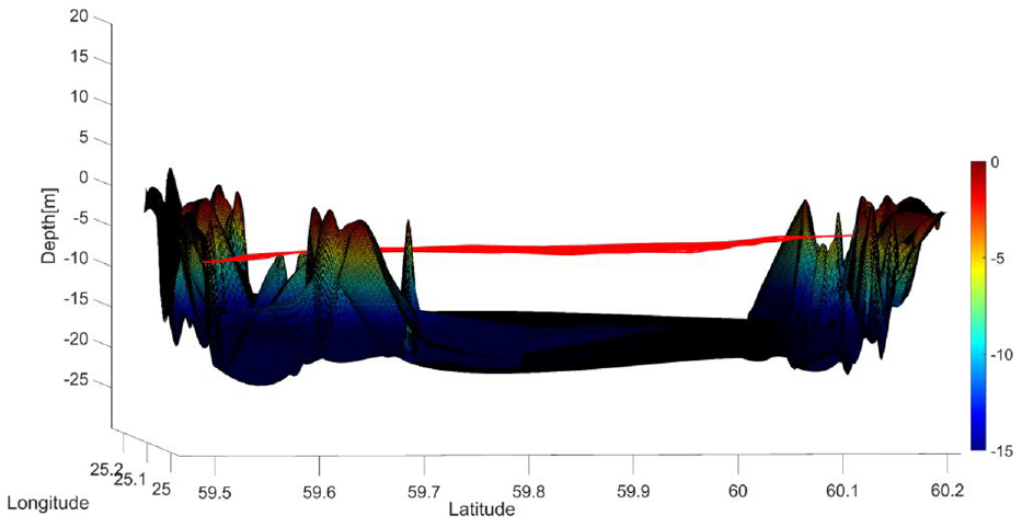
Ship voyages from Helsinki to Tallinn.

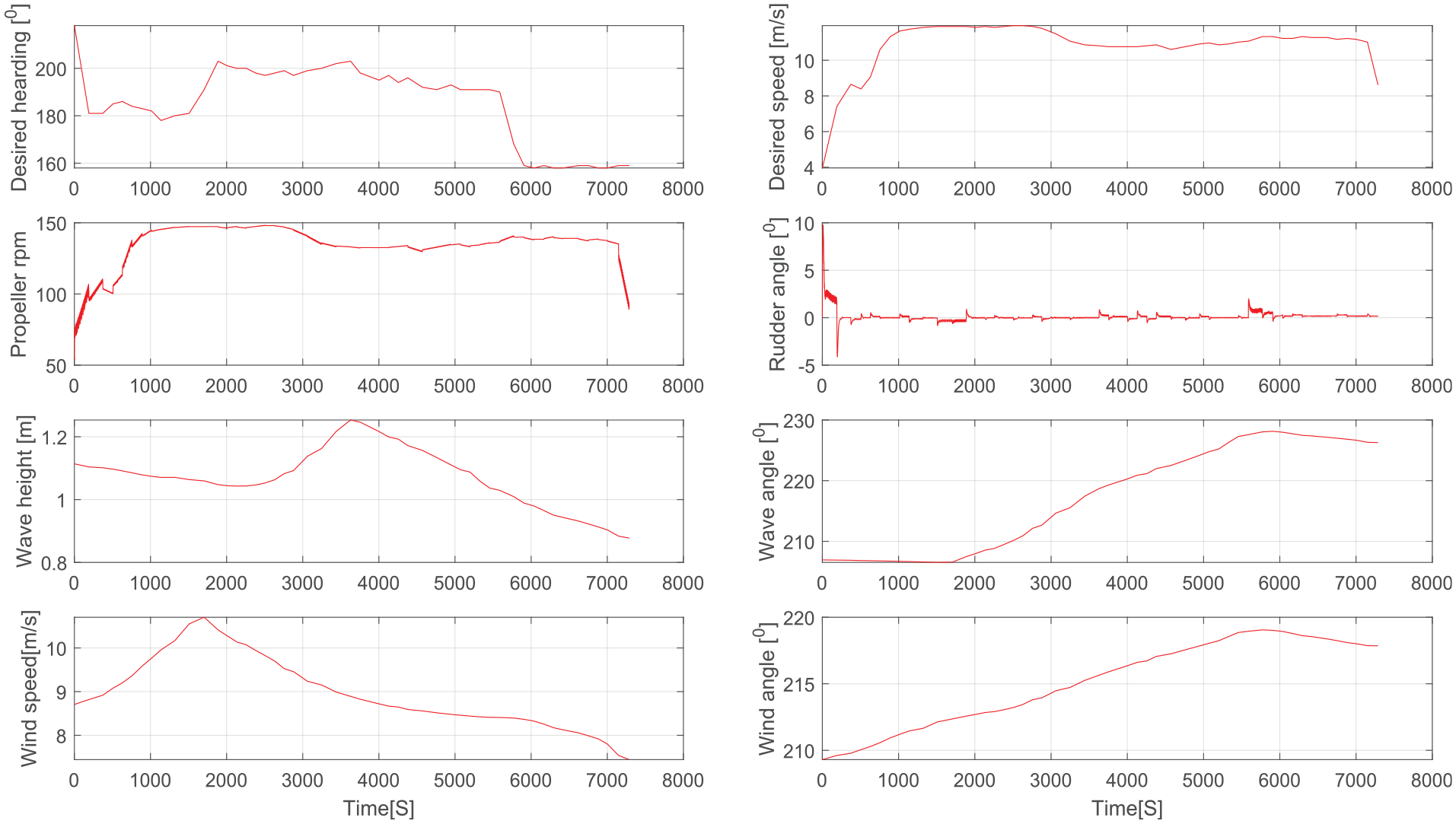
In framing up the environmental conditions for these voyages, both ship location and hydro-meteorological data history records from now-cast records were considered, as shown in Section (Ship motion features extraction). Consequently, the desired speed and heading angle, the encountered hydro-meteorological conditions, and water depth were extracted, as shown in Figure 10. These voyage and environmental data were used to generate 6-DoF ship motion dynamics (6-DoF ship motion dynamics simulation).

Figure 10.

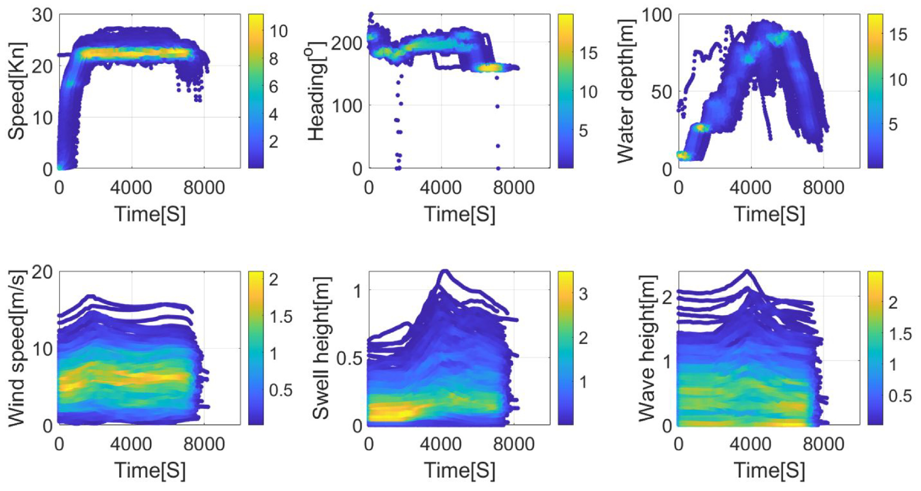
Time domain operational conditions for each voyage from departure to destination (the x-axis denotes the time from departure port to destination port).

6-DoF ship motion dynamics simulation

Time domain input conditions used in simulations were gathered from the detailed assessment of AIS, GEBCO, and now-cast data, according to the method presented in Section (Extracting ship motion features in real conditions). The rock profile nearby the selected Helsinki to Tallin route was extracted from GEBCO data. The seabed profile was idealised by multiple conical rocks with a rounded tip radius. The seafloor has a large profile that changes across tens of kilometres. A multiple conical rock model was employed to take this geometry into consideration. The detail of rock profile modelling is given in Figure 11, by Taimuri et al.⁴⁹ Only those seabed profiles were considered, where the tip of the rock from the mean sea surface is less than the ship’s approximate design draft (=7.5 m). These rock points are in the shallow water region, as highlighted in Figure 12.

Figure 11.

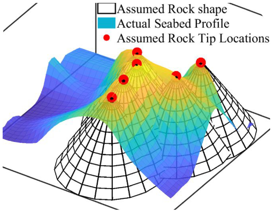
Rock model and seabed profile. The idealisation of the seabed is formed using multiple conical rocks with a rounded tip radius.

Figure 12.

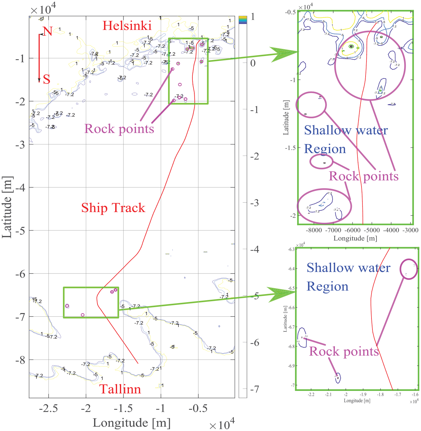
Rock identification in the region from Helsinki to Tallinn. Real ship track is shown from AIS data, corresponding to nearby shallow water regions and rock tips.

According to the process of Section (6-DoF FSI ship grounding dynamics model), environmental actions, real-time rudder angles, propeller rpm, thrust, and 6-DoF ship motions were embedded in the ship dynamics model (e.g. see results for a selected case in Figure 13). This shows that the PD- and P-controller satisfactorily judge the ship track and can be used to identify the rudder angle. The detailed mathematical modelling of internal and external mechanics, input conditions and validation cases can be found in Taimuri et al.^7,33,49,50.

Figure 13.

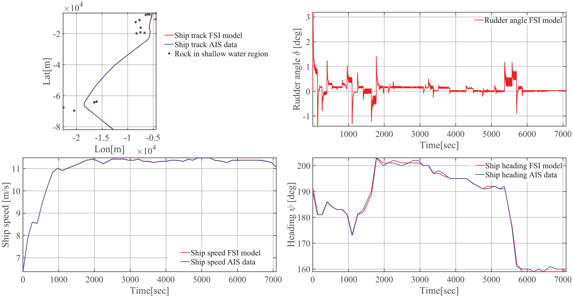
Generating the results from the physics-based model FSI model.

6-DoF ship motion dynamics prediction using Deeping Learning

Based on the obtained ship motion features and environmental conditions, the 6-DoF ship dynamics model was used to generate the time domain input parameters (rudder angle, propeller rpm) and time domain output results (6-DoF ship motion dynamics) for 500 voyages between Helsinki and Tallin (6-DoF ship motion dynamics simulation). Then, a transformer architecture was designed to train a deep learning model by mapping the context {X} to context {Y} (see Ship motion dynamics estimation transformer).

Ship motion dynamics prediction transformer

In this paper, the total data set was split into 80% (for training), 10% (for validation) and 10% (for testing) over 500 voyages in total. The training data set included 400 ship voyages. The validation and testing data sets had 50 ship voyages (see Figure 16). Computations were carried out on the high-performance computing platform of the Centre for Science (CSC) of Finland. To train a ship motion dynamics prediction model, the number of the epoch was set to 60. The training loss and validation loss were calculated based on the training and validation data set. The curves presented in Figure 14 show that the training and validation loss decrease and stabilise at the epoch of 38. The training process results indicate that the deep learning model is an optimal fit (i.e. it does not over - or under–fit).

Figure 14.

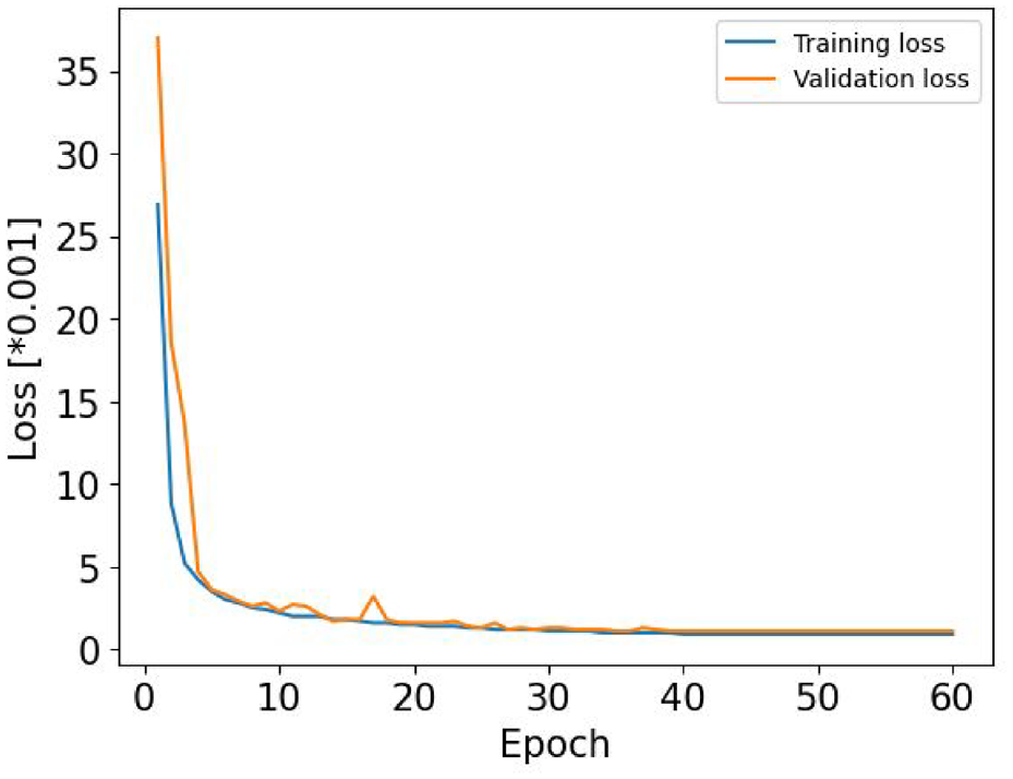
The model performance evaluation.

The training dataset is generally set as 70%–90% of the total data.² To better understand the difference in data selection for training a high-performance transformer model, the validation loss was calculated based on different percentages of the total data set (see Figure 15). The validation dataset was set as 10% of the total data. The same validation dataset was used to evaluate the trained model albeit using various lengths of training data sets. The results indicate that the training loss decrease as the training set increases, and when the training data set exceed 57% of the total data set (285 voyages), the training error tends to be stable. The analysis indicates that more than 285 voyages are recommended to train the 6-DoF ship motion prediction model using the proposed method.

Figure 15.

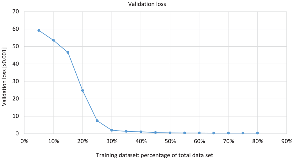
The influences of different lengths of training data sets on validation loss evaluation.

The trained deep learning model was used to predict ship motion dynamics between two ports as well as the turning circle. Although the training data (context {X} to context {Y}) were extracted from various voyages, the model utilised inputs (stable rudder angle) for the prediction of the turning circle of the ship herself (see Figure 16).

Figure 16.

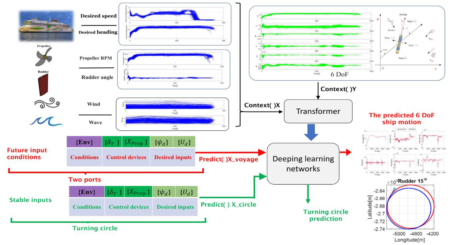
The deep learning processing of 6-DoF ship motion prediction for the long-term voyage in real conditions and turning circle in calm conditions.

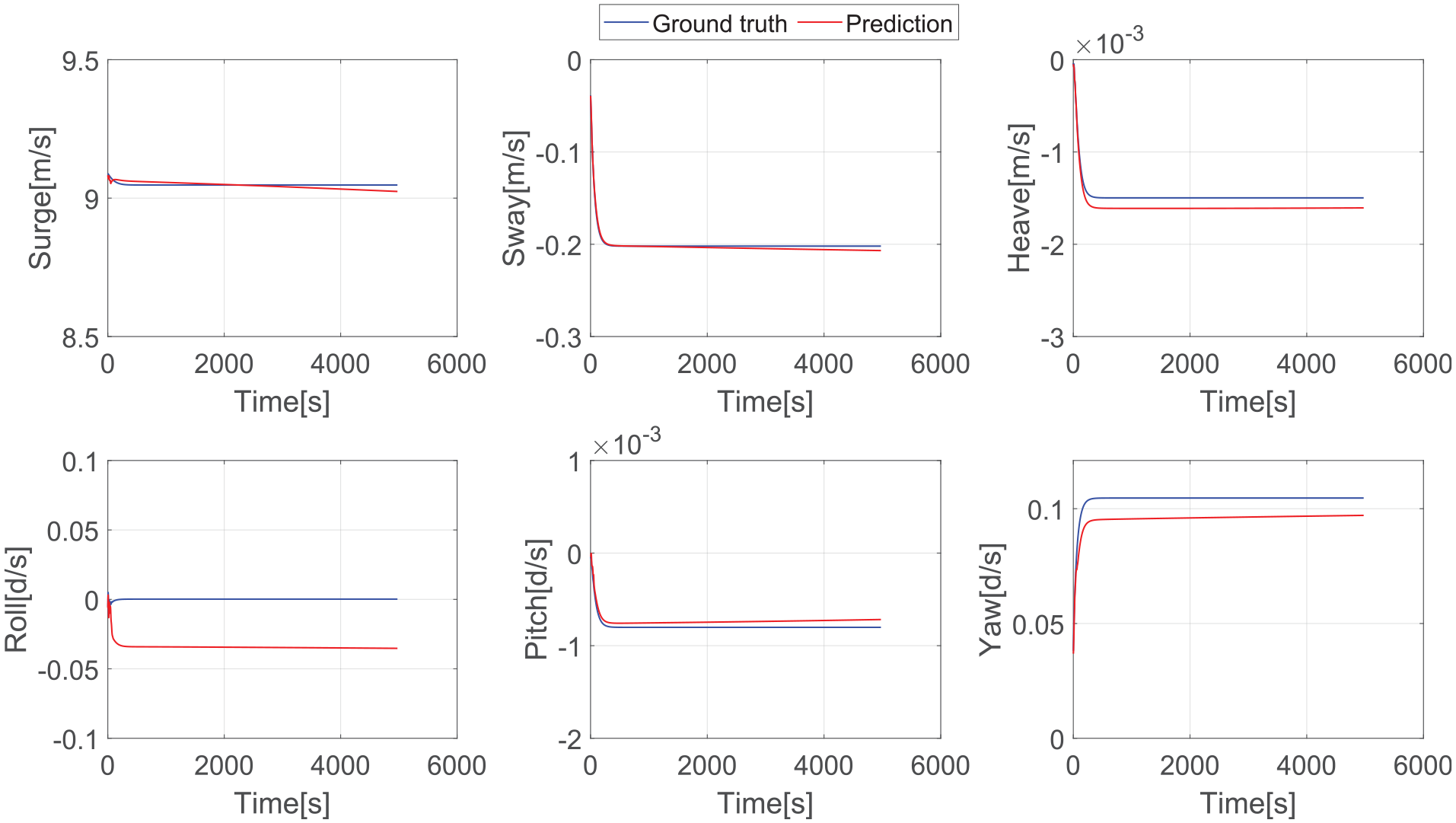
To test the trained deep learning model, the future inputs of the ship control action, desired inputs and environmental conditions were regarded as the predicted {X}_voyage (see Figure 17). The 6-DoF ship motions were predicted, as shown in Figure 18. These results indicate that the trained deep learning model can capture the ship motion features in real conditions.

Figure 17.

Input conditions for the validation of the trained model.

Figure 18.

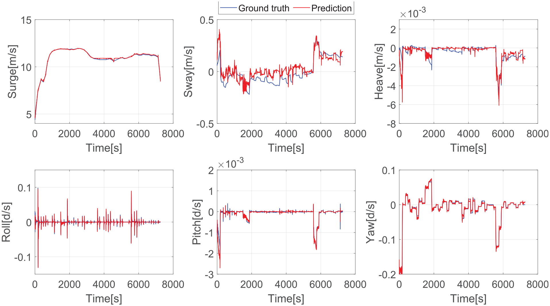
The results of the prediction of ship motion dynamics (the ground truth represents the real data in blue; the prediction denotes the predicted results in red.).

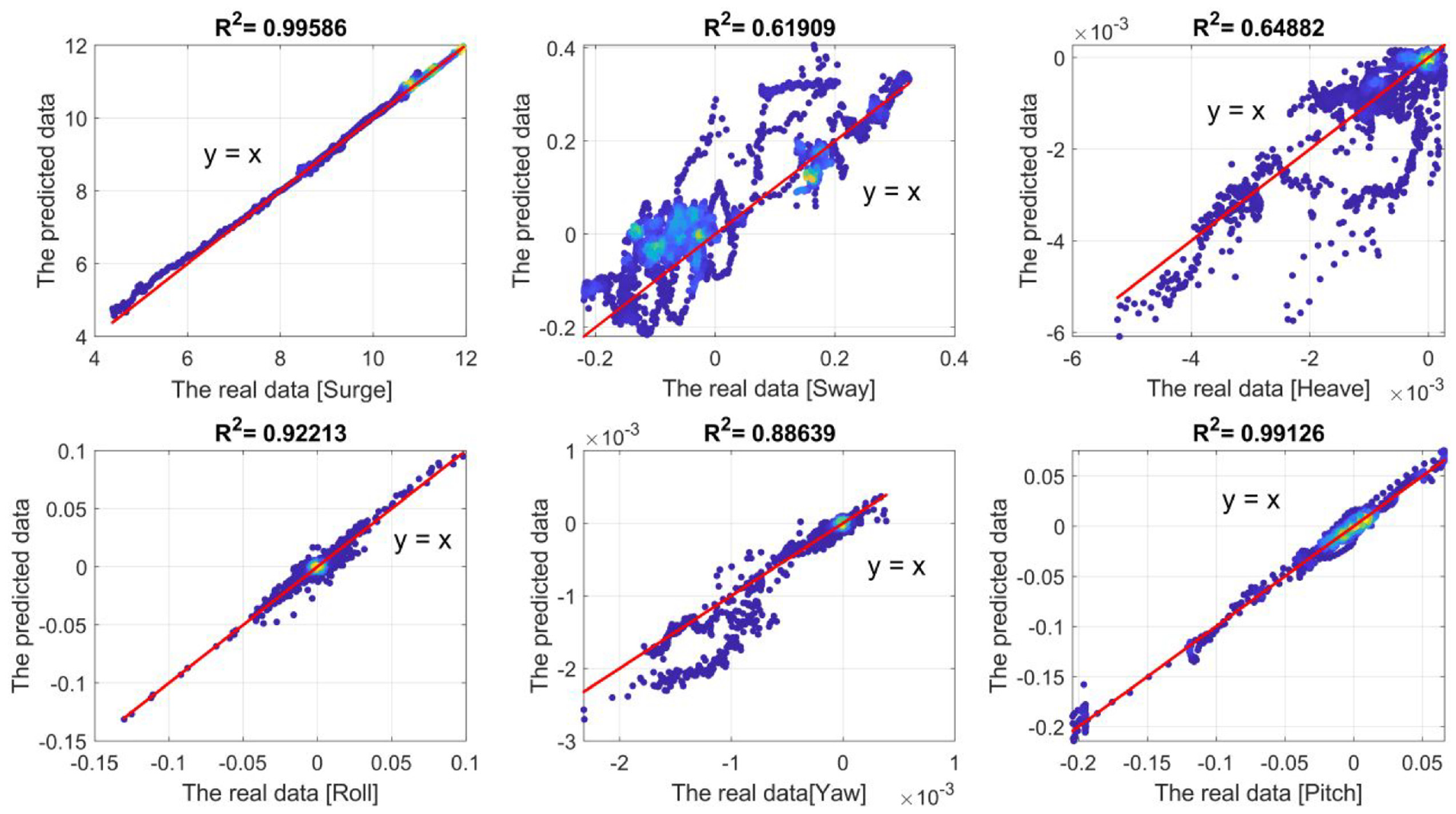
To precisely evaluate the performance of the trained model, $R^{2}$ values were evaluated (see Figure 19). The $R^{2}$ values of the prediction of the surge, roll, and pitch are more than 0.9. The $R^{2}$ values of the prediction of sway and heave are 0.62 and 0.65. The results indicate that the predicted and real values are close. The model is good in terms of predicting all 6 – DoF motions. However, agreement against sway and heave predictions is slightly worse than surge, roll, and pitch. This may be because the adopted method is based on an auto-regression model that underestimates some influencing factors in ship sway and heave (e.g. swell, current etc.).

Figure 19.

The results of the performance evaluation using $R^{2}$ .

Errors evaluation and comparison studies

Following the testing of data sets, comparisons of the existing deep learning methods are demonstrated in Table 3. The Gate Recurrent Unit (GRU) and Long-Short Term Memory (LSTM) are typical deep learning methods for time series prediction.^51,52 GRU and LSTM were adopted to predict ship motions, see more in Li et al.⁵³ and Zhang et al.⁵⁴ The results show that the prediction errors are higher than those from the proposed method. For the datasets available, the RMSE and MAE were calculated for the prediction of 6-DoF ship motions using GRU, LSTM and the proposed method, as shown in Table 3. This indicates that the errors of the proposed method are the lowest, and the proposed method presents encouraging outputs, which are suitable for predicting 6-DoF ship motion dynamics accounting for ship control devices in real operational conditions. The reasons behind these observations are as follows: (1) LSTM and GRU are sequential models and, therefore, may capture ship motions in the time domain. They are limited in terms of learning more features from long-term sequences of ship motions, and their parallelisation ability also is limited⁵⁵; (2) The transformer model overcomes the disadvantages of LSTM and GRU and relies entirely on self-attention to calculate representations of ship motion sequences in the time domain without using sequence-aligned convolution.^43,46 Based on the attention mechanism, the parallelisation ability gets promoted, and much more data streams can be processed simultaneously with transformer-based models. These advantages help the proposed model to cope efficiently with long sequences and improve the accuracy of ship motion predictions.

Table 3.

The accuracy evaluation for 6-DoF ship motion prediction using various tools.

Methods	Error	Surge	Sway	Heave	Roll	Yaw	Pitch
Transformer	MAE	0.0529	0.0599	0.0003	0.001	0.0001	0.0026
Transformer	RMSE	0.0745	0.0734	0.0004	0.0021	0.0001	0.0037
GRU	MAE	1.0536	0.1014	0.0007	0.0022	0.0004	0.0627
GRU	RMSE	1.3876	0.1113	0.0008	0.0026	0.0005	0.0747
LSTM	MAE	0.4936	0.099	0.001	0.0054	0.0005	0.013
LSTM	RMSE	0.4959	0.1173	0.001	0.0055	0.0005	0.0161

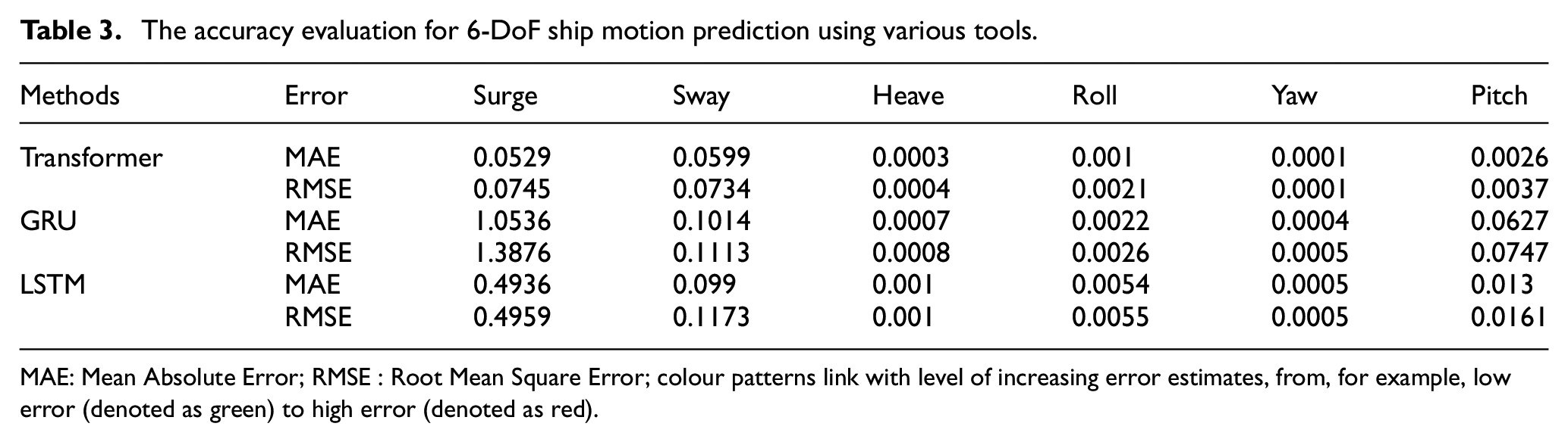
MAE: Mean Absolute Error; RMSE : Root Mean Square Error; colour patterns link with level of increasing error estimates, from, for example, low error (denoted as green) to high error (denoted as red).

Ship turning circle prediction

The results presented in Section (Errors evaluation and comparison studies) show that the trained deep learning neural network can accurately capture ship motion dynamics in real conditions. To better highlight the generalisation ability of this trained model, ship motion dynamics are predicted by setting stable rudder angles as new inputs to generate a turning circle. The stable rudder angles are set as 1°, 5°, 10° and 15° (starboard), and the propeller revolutions are set as 109 rpm. As shown in Figure 20, the 6-DoF ship motion dynamics are predicted while the rudder angle is set to 1° for a starboard turn.

Figure 20.

The results of the prediction of ship turning circle (Rudder angle = 1°, Starboard; Propeller rpm = 109).

Figure 21 presents the prediction of turning circles with various rudder angles (Rudder angles = 1°, 5°, 10°, 15°). It is shown that the trained deep learning model also captures the turning feature of the ship herself. The trained data streams do not include the data of a ship turning circle. Yet results indicate that the model is capable of “learning” the ship manoeuvring features. In conclusion, the generalisation ability of the trained model is very good, and the trained model also has good performance in terms of reacting to new data and making accurate predictions.

Figure 21.

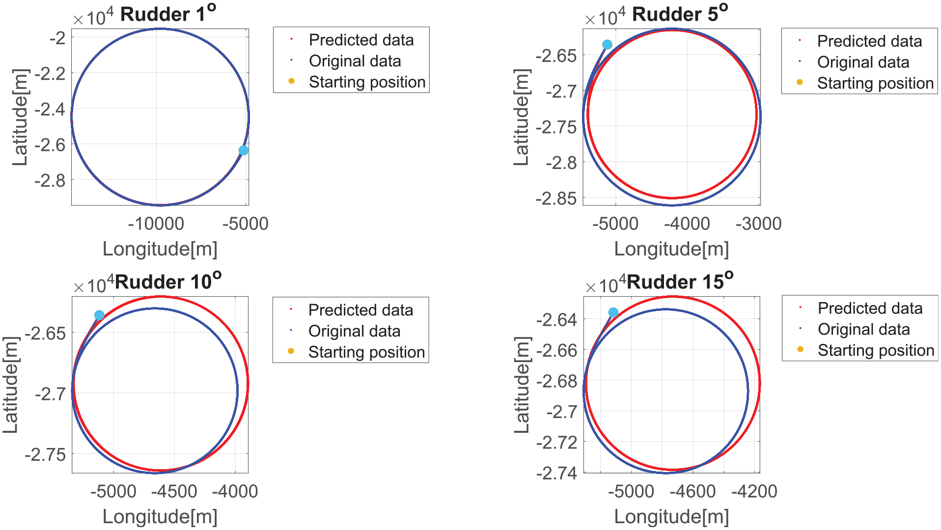
The results of the prediction of ship turning circle with various rudder angles.

An error analysis of turning circle predictions for various rudder angles (Rudder angle = 1°, 5°, 10°, 15°) is given in Figure 22. The results indicate that the predicted error increases with the increased rudder angle. This is because 96.8% of rudder angles in trained datasets are in the interval [−1°, 1°] (see Figure 23). With the increase of rudder angle, the number of training data decreases, leading to low accuracy of turning circle prediction for high rudder angles. Thus, more complex voyages with ship motion dynamics in real conditions can be trained using the proposed method to improve the accuracy of the turning circle prediction for high rudder angles.

Figure 22.

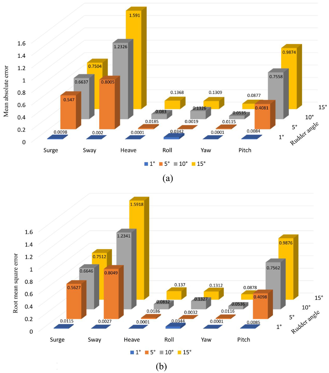
The error analysis of turning circle prediction at different rudder angles: (a) Mean absolute error analysis for turning circle prediction. (b) Root mean square error analysis for turning circle prediction.

Figure 23.

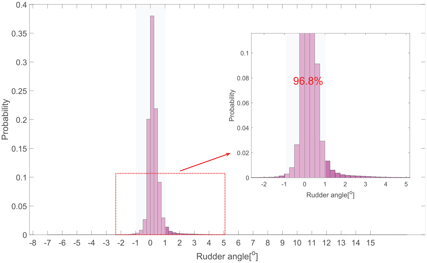
The distribution of the rudder angles of the trained data. The window demonstrates that distribution ranges from [−1 to 1].

Conclusions

This paper introduced a deep learning method to predict 6-DoF ship dynamics in real conditions. The proposed deep learning method accounted for (1) ship motion features and environmental conditions extraction; (2) 6-DoF ship dynamics; (3) the training of deep learning neural networks to capture the ship motion features. The method is demonstrated by focusing on the Ro - Pax ship, sailing from Tallin to Helsinki. In total 500 voyages of the selected ship were used to train, validate or test the model. Results indicate that the proposed method can predict (1) 6-DoF ship motion dynamics in real conditions between two ports and (2) ship turning circles with various rudder angles in calm conditions. At this stage, the proposed framework has limitations in terms of reflecting actual ship operations in real sea states. The trained model could be evaluated by using the data from sea trials with more focus on various ship segments.

Footnotes

Acknowledgements

Special thanks of appreciation go to CSC Finland for the provision of their parallel computing facilities. The views set out in this paper are those of the authors and do not necessarily reflect the views of their sponsors.

Declaration of conflicting interests

The author(s) declared no potential conflicts of interest with respect to the research, authorship, and/or publication of this article.

Funding

The author(s) disclosed receipt of the following financial support for the research, authorship, and/or publication of this article: Part of the research presented in this paper has received funding from European Union project FLooding Accident REsponse (FLARE) number 814753, under H2020 programme. The authors express their gratitude for this support and the selected sponsorships received from Merenkulun Säätiö (No. 20220071, 20220072, 20220073).

ORCID iDs

Mingyang Zhang

Ghalib Taimuri

Jinfen Zhang

Notes

References

Hirdaris

Mikkola

eds. Ship dynamics for performance based design and risk averse operations. Journal of Marine Science and Engineering, 2021.

Zhang

Kujala

Musharraf

, et al. A machine learning method for the prediction of ship motion trajectories in real operational conditions. Ocean Eng, Under review, 2022.

Zhang

Zou

ZJ.

Identification of Abkowitz model for ship manoeuvring motion using ε-support vector regression. J Hydrodyn 2011; 23(3): 353–360.

Zhang

Liu

Wan

, et al. Experimental and numerical investigations of advancing speed effects on hydrodynamic derivatives in MMG model, part I: Xvv, Yv, Nv. Ocean Eng 2019; 179: 67–75.

Chillcce

el Moctar

A numerical method for manoeuvring simulation in regular waves. Ocean Eng 2018; 170: 434–444.

Tillig

Ringsberg

JW.

A 4 DOF simulation model developed for fuel consumption prediction of ships at sea. Ships Offshore Struct 2019; 14(suppl 1): 112–120.

Taimuri

Matusiak

Mikkola

, et al. A 6-DoF maneuvering model for the rapid estimation of hydrodynamic actions in deep and shallow waters. Ocean Eng 2020; 218: 108103.

Gil

Montewka

Krata

, et al. Determination of the dynamic critical maneuvering area in an encounter between two vessels: operation with negligible environmental disruption. Ocean Eng 2020; 213: 107709.

Gil

A concept of critical safety area applicable for an obstacle-avoidance process for manned and autonomous ships. Reliab Eng Syst Saf 2021; 214: 107806.

10.

Soares

CG.

Convergence analysis of hydrodynamic coefficients estimation using regularisation filter functions on free-running ship model tests with noise. Ocean Eng 2022; 250: 111012.

11.

Okuda

Yasukawa

Sano

, et al. Maneuvering simulations of twin-propeller and twin-rudder ship in shallow water using equivalent single rudder model. J Marine Sci Technol 2022; 1–23.

12.

Cheng

Liu

, et al. Maneuvering modeling of a twin-propeller twin-rudder inland container vessel based on integrated CFD and empirical methods. Appl Ocean Res 2022; 126: 103261.

13.

Ramirez

Leong

Nguyen

, et al. Non-parametric dynamic system identification of ships using multi-output Gaussian processes. Ocean Eng 2018; 166: 26–36.

14.

Wang

Zou

Soares

CG.

Identification of ship manoeuvring motion based on nu-support vector machine. Ocean Eng 2019; 183: 270–281.

15.

Zeng

Xia

Cai

Parameter identification of hydrodynamic model of ship using EKF. In: 2021 China Automation Congress (CAC), 2021October, pp. 1427–1432. New York: IEEE.

16.

Silva

Maki

KJ.

Data-driven system identification of 6-DoF ship motion in waves with neural networks. Appl Ocean Res 2022; 125: 103222.

17.

Ouyang

Zou

ZJ.

Nonparametric modeling of ship maneuvering motion based on Gaussian process regression optimised by genetic algorithm. Ocean Eng 2021; 238: 109699.

18.

Woo

Kim

Deep reinforcement learning-based controller for path following of an unmanned surface vehicle. Ocean Eng 2019; 183: 155–166.

19.

Sivaraj

Rajendran

Prasad

LP.

Data driven control based on Deep Q-Network algorithm for heading control and path following of a ship in calm water and waves. Ocean Eng 2022; 259: 111802.

20.

Lou

Wang

, et al. Deep learning method for 3-DOF motion prediction of unmanned surface vehicles based on real sea maneuverability test. Ocean Eng 2022; 250: 111015.

21.

Hexeberg

Flåten

Brekke

EF.

AIS-based vessel trajectory prediction. In: 2017 20th international conference on information fusion (Fusion), 2017, July, pp. 1–8. New York: IEEE.

22.

Alizadeh

Alesheikh

Sharif

Vessel trajectory prediction using historical automatic identification system data. J Navigat 2021; 74(1), 156–174.

23.

Lian

Yang

, et al. Research on Ship AIS Trajectory Estimation Based on Particle Filter Algorithm. In: 2019 11th International conference on intelligent human-machine systems and cybernetics (IHMSC), 2019August, Vol. 1, pp. 305–308. New York: IEEE.

24.

Rong

Teixeira

Soares

CG.

Ship trajectory uncertainty prediction based on a Gaussian Process model. Ocean Eng 2019; 182: 499–511.

25.

Liu

Xie

, et al. (2020, October). Predicting the trajectories of vessels using machine learning. In: 2020 5th International conference on control, robotics and cybernetics (CRC), pp. 66–70. New York: IEEE.

26.

Virjonen

Nevalainen

Pahikkala

, et al. Ship movement prediction using k-NN method. In: 2018 Baltic Geodetic Congress (BGC Geomatics), 2018, June, pp. 304–309. IEEE.

27.

Liu

Jiang

, et al. TPR-DTVN: a routing algorithm in delay tolerant vessel network based on long-term trajectory prediction. Wireless Commun Mobile Comput 2021; 2021: 1–15.

28.

Forti

Millefiori

Braca

, et al. Prediction oof vessel trajectories from AIS data via sequence-to-sequence recurrent neural networks. In: ICASSP 2020-2020 IEEE International Conference on Acoustics, Speech and Signal Processing (ICASSP), 2020May, pp. 8936–8940. New York: IEEE.

29.

Wang

Ren

Vessel trajectory prediction based on AIS data and bidirectional GRU. In: 2020 International conference on computer vision, image and deep learning (CVIDL), 2020July, pp. 260–264. New York: IEEE.

30.

Nguyen

Fablet

TrAISformer-A generative transformer for AIS trajectory prediction. arXiv preprint arXiv:2109.03958, 2021.

31.

Nguyen

Fablet

RT.

A generative transformer for AIS trajectory prediction. arXiv 2019. ArXiv preprint arXiv:2109.03958.

32.

Lam

JSL

Yang

, et al. Unsupervised hierarchical methodology of maritime traffic pattern extraction for knowledge discovery. Transp Res C Emerg Technol 2022; 143: 103856.

33.

Taimuri

Kim

Mikkola

, et al. A two-way coupled FSI model for the rapid evaluation of accidental loads following ship hard grounding. J Fluids Struct 2022a; 112: 103589.

34.

Zhang

Montewka

Manderbacka

, et al. A big data analytics method for the evaluation of ship-ship collision risk reflecting hydro-meteorological conditions. Reliab Eng Syst Saf 2021; 213: 107674.

35.

Liu

Nie

Garg

, et al. Data-driven trajectory quality improvement for promoting intelligent vessel traffic services in 6G-enabled maritime IoT systems. IEEE Internet Things J 2020; 8(7): 5374–5385.

36.

Liang

Liu

Zhan

, et al. Fine-grained vessel traffic flow prediction with a spatio-temporal multigraph convolutional network. IEEE Trans Intell Transp Syst 2022; 23(12): 1–14.

37.

Hirdaris

Zhang

Montewka

, et al. Analysis of routing and traffic data, EU Project FLARE WP2, Deliverable Report D2.4, https://flare-project.eu/images/downloads/191028_FLARE_Deliverable_2.2_Final.pdf (2019, accessed 13 June 2022)

38.

Zhang

Kujala

Hirdaris

A machine learning method for the evaluation of ship grounding risk in real operational conditions. Reliab Eng Syst Saf 2022; 226: 108697.

39.

Blendermann

Parameter identification of wind loads on ships. J Wind Eng Ind Aerodyn 1994; 51(3): 339–351.

40.

Matusiak

Dynamics of a Rigid Ship-with applications. Espoo, Finland: Aalto University, 2021.

41.

Le Cun

Bengio

Hinton

. Deep learning. Nature 2015; 521(7553): 436–444.

42.

Goodfellow

Bengio

Courville

Deep learning. Cambridge: MIT Press, 2016.

43.

Vaswani

Shazeer

Parmar

, et al. Attention is all you need. Adv Neural Inform Proc Sys 2017; 30: 5998–6008.

44.

Han

Xiao

, et al. Transformer in transformer. Adv Neural Inform Proc Syst 2021; 34: 15908–15919.

45.

Parmar

Vaswani

Uszkoreit

, et al. Image transformer. In: International conference on machine learning. PMLR, 2018, pp. 4055–4064. Stockholm SWEDEN

46.

Khan

Naseer

Hayat

, et al. Transformers in vision: a survey. ACM Computing Surveys 2022; 54(10s): 1–41.

47.

Bhattacharya

Petrangeli

, et al. Show Me What I Like: Detecting user-specific video highlights using content-based multi-head attention. arXiv preprint arXiv:2207.08352, 2022.

48.

Liu

, et al. Neural speech synthesis with transformer network. In: Proceedings of the AAAI Conference on Artificial Intelligence, Vol. 33, No. 01, 2019July, pp. 6706–6713. Honolulu, Hawaii, USA

49.

Taimuri

Ruponen

Hirdaris

A novel method for the probabilistic assessment of ship grounding damages and their impact on damage stability. Struct Saf (Under review), 2022.

50.

Taimuri

Zhang

Hirdaris

A predictive analytics method for the avoidance of ship grounding in real operational conditions. In: SNAME maritime convention26–29 September 2022, p. 18, Houston, TX. https://doi.org/10.5957/SMC-2022-012

51.

Cho

Van Merriënboer

Bahdanau

, et al. On the properties of neural machine translation: Encoder-decoder approaches. arXiv preprint arXiv:1409.1259, 2014.

52.

Gers

Schmidhuber

Cummins

Learning to forget: continual prediction with LSTM. Neural Comput 2000; 12(10): 2451–2471.

53.

Geng

, et al. A ship motion forecasting approach based on empirical mode decomposition method hybrid deep learning network and quantum butterfly optimisation algorithm. Nonlinear Dyn 2022; 107(3): 2447–2467.

54.

Zhang

Zheng

Liu

MX.

Multiscale attention-based LSTM for ship motion prediction. Ocean Eng, 2021; 230: 109066.

55.

Zeyer

Bahar

Irie

, et al. A comparison of transformer and lstm encoder decoder models for ASR. In: 2019 IEEE Automatic Speech Recognition and Understanding Workshop (ASRU), 2019, December, pp. 8–15. New York: IEEE.

A deep learning method for the prediction of 6-DoF ship motions in real conditions

Abstract

Keywords

Introduction

Methods

Ship motion features extraction

6-DoF FSI ship grounding dynamics model

Ship motion dynamics estimation transformer

Attention mechanism/multi-head attention layer

Add and Norm layers

Feed-forward network

Linear layer

Case studies

Extracting ship motion features in real conditions

6-DoF ship motion dynamics simulation

6-DoF ship motion dynamics prediction using Deeping Learning

Ship motion dynamics prediction transformer

Errors evaluation and comparison studies

Ship turning circle prediction

Conclusions

Footnotes

Acknowledgements

Declaration of conflicting interests

Funding

ORCID iDs

Notes

References