
Abstract
Fluid-filled pipelines are widely used in engineering and industry. An analysis of the frequency dynamic responses of three-dimensional pipes is presented in this paper. A general formulation is developed based on an impedance matrix transmission approach in which a T-shaped pipe system can be assembled from three straight pipes. For validation purposes, numerical results are compared with data given by finite element method (FEM) software, previous literature, and an experiment. In the experiment, the three-dimensional pipe system is suspended horizontally on spring wires and is excited in the X and Y directions. It is found that the results calculated using the proposed method match the experimental results well. A dimensionless analysis of Poisson’s coupling is then carried out, and the junction coupling of the branch pipe is analyzed as a function of its angle. Through this work, it is shown that the proposed method is efficient and can be used to predict the vibration of three-dimensional pipes.
Keywords
Introduction
The fluid-filled pipeline system is very important in many engineering fields, such as marine craft 1 and airplanes. 2 The vibration of such pipelines can cause damage to devices mounted on the pipe systems. 3 Hence, much research has focused on the development of suitable methods to predict the dynamic responses of fluid-filled pipe systems.4,5 One of the basic pipeline systems is the T-shaped pipe, which can be used to split and combine flows. 6 At the junction, interactions between the fluid and structure can induce pipe wall vibrations and fluid pressure fluctuations.
Lee and Kim 7 introduced a finite element formulation for the fully-coupled dynamic equations of such a system and applied it to several sample pipeline systems. The numerical results were validated by comparison with those given in reference work. The numerical results showed that the nonlinear coupling terms may become significant at high pressures and velocities. Liu et al. 8 proposed an absorbing transfer matrix method in the frequency domain for fluid-filled pipelines with various branched pipes. Several cases were studied to illustrate the application of the proposed method. The effects of various parameters were analyzed and it was found that the fluid pressure and vibration can be optimized by changing the branch angles and positions. Li et al. 9 modified the original four-equation model for a pipe conveying fluid by taking the dynamic effects of the fluid into account. The proposed method was applied to calculate the first three natural frequencies of a three-span pipe 12 m long in three different cases. It was found that the dynamic stiffness method could still provide high precision even for a relatively large element size. Tijsseling and Vardy10,11 experimentally studied the fluid-structure interactions (FSI) in a T-junction pipe, which is a closed, water-filled, T-shaped laboratory pipe system. The results showed that coupling at boundaries and wavefront propagation along a pipe can have a major influence on stress and pressure histories. Xu et al. 12 used the transfer matrix method to describe fluid-structure interactions in liquid-filled pipes. A general solution was proposed to predict the frequency response of a multi-branch piping system. Gomes da Rocha and Bastos de Freitas Rachid 13 presented a numerical procedure involving advancing in time sequentially through these sets of equations by employing Glimm’s method and Gear’s stiff method. Very good agreement was found between numerical results obtained from this method and experimental data. Pérez-García et al. 14 developed a methodology based on the calculation of thermo-fluid properties extrapolated to the branch axes intersection to obtain the total pressure loss coefficient in the internal flow in a T-shaped junction.
In a special pipe system, Tentarelli 15 obtained a solution of the 14-equation model using the transfer matrix method (TMM) and compared the theoretical prediction for a three-dimensional pipe system with an elbow and a tee with an experiment in both the time and frequency domains. Craggs and Stredulinsky 16 established a two-dimensional finite element model of a pipe system consisting of bends and “cross” and “tee” junctions. Guangbin et al. 17 experimentally studied the characteristics of two-phase flow in a Y-shaped branch pipe. Walker et al. 18 investigated T-type junctions using numerical simulations. Other researchers, including Kriesels et al. 19 and Ziada and Shine, 20 reported flow-induced pulsations in pipe systems with closed side branches.
Compared with experimental and numerical simulation methods, analytical methods are simple, fast, and low-cost. The accuracy, applicability, and efficiency of an analytical model for a pipeline system determine its value in theoretical research and engineering applications. As seen above, much attention has been paid to straight and curved fluid-filled pipes, but more complicated three-dimensional pipe systems with multiple branches still need to be intensively investigated. In this paper, the impedance synthesis method (ISM) is introduced to study the dynamic response of a three-dimensional pipe system. For validating the developed method, numerical results are compared with those given by FEM simulations and experiment. The greatest advantage of the ISM is that, when an analytical solution cannot be obtained for pipe components, such as for a rubber hose, muffler, or elastic support, their impedance matrices can be obtained from experimental data instead, which is easier to obtain than a transfer matrix. These test impedance matrices can then be inserted into the overall pipe system impedance matrix. The proposed method could help to provide some physical insight into the interactions between pipeline systems and fluid, and offers a certain degree of flexibility to the low-noise design of pipeline systems.
Vibration governing equation
The variables and forces associated with a straight fluid-filled pipe can be seen in Figure 1.
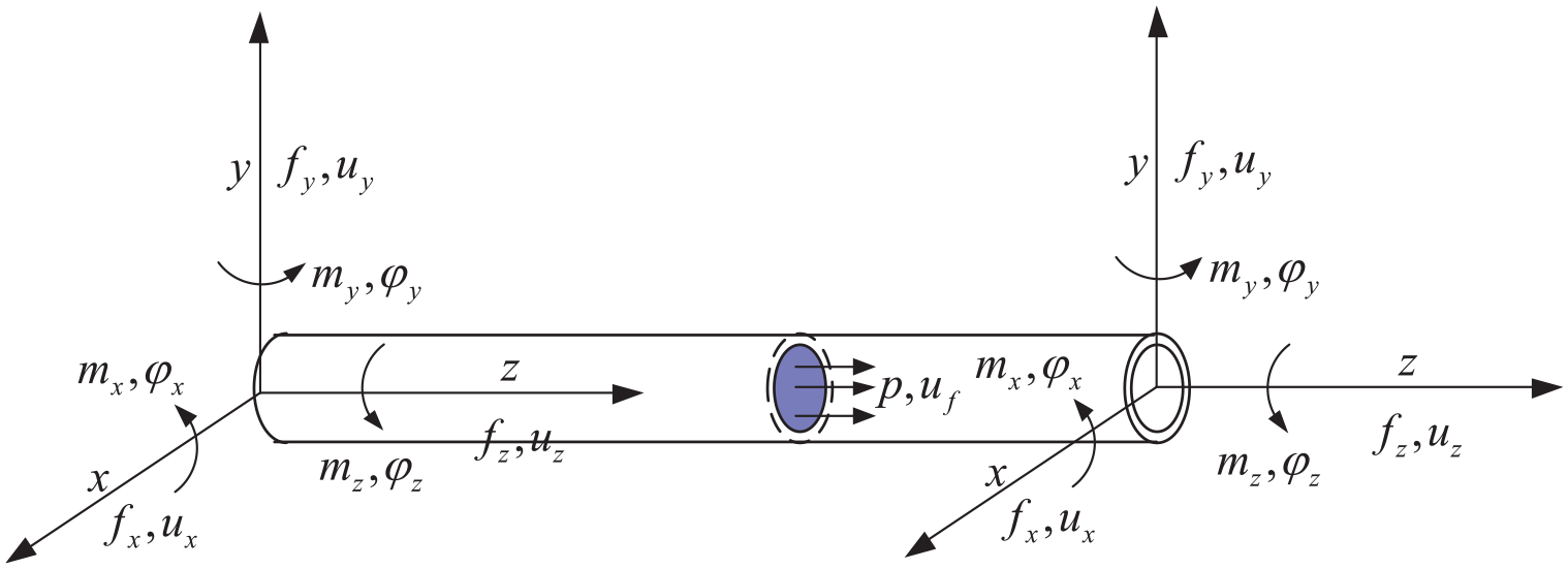
Variables and forces of a straight fluid-filled pipe.
Axial vibration impedance
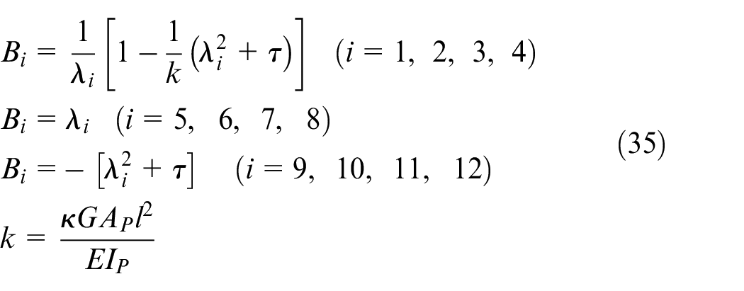
For the fluid-filled Timoshenko beam model, the governing vibration equation including the liquid pressure and displacement, axial pipe stress, and displacement can be written as 21 :
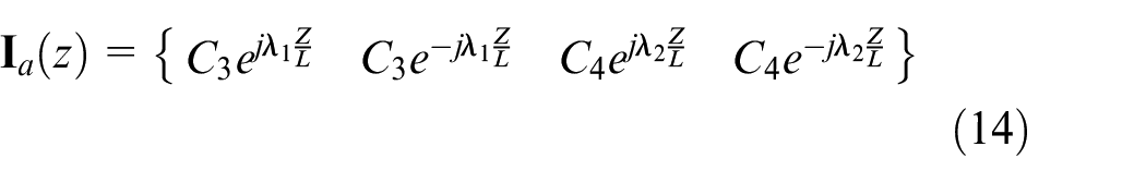
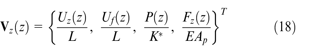
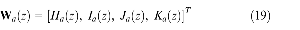
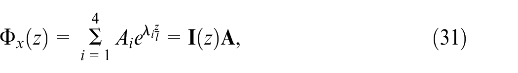
There are four variables,
where
To make it dimensionless, both sides of equation (3) can be divided by
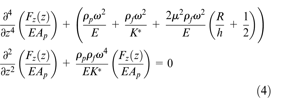
According to the superposition principle of the wave propagation method, the solution of equation (4) can be written as:
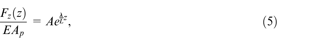
where

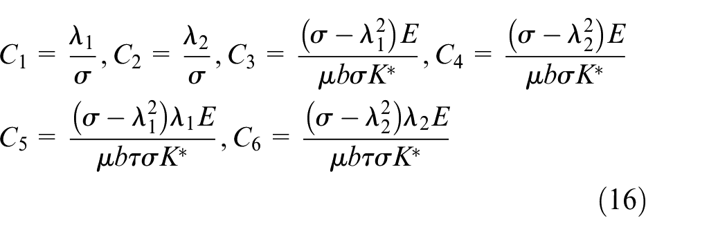
The roots of equation (6) can be written as:
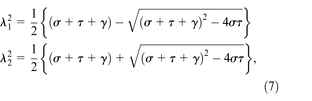
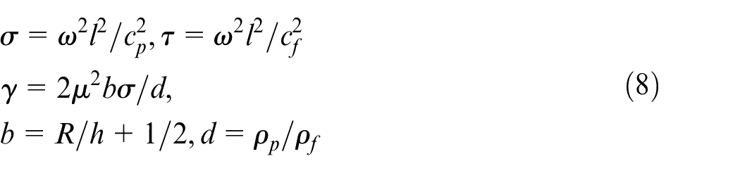
where:
Thus, according to equation (5), the solution of equation (4) can be written as:
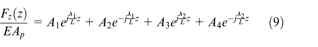
If we assume
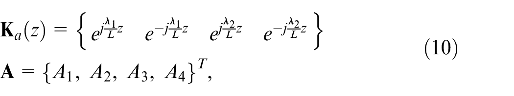
we can obtain:

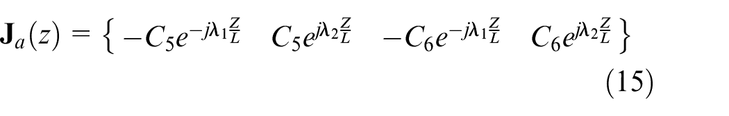
Substituting equation (11) into equation (1), the other three unknown variables can be written as:
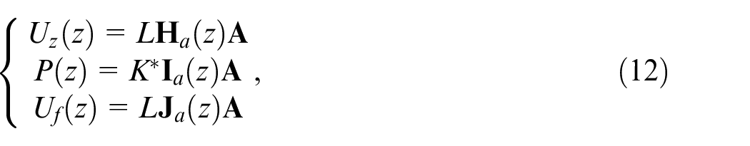
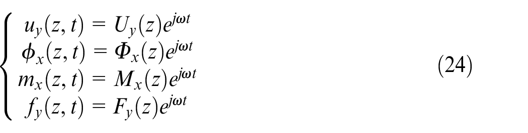
where:
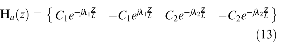
and
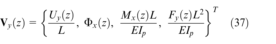
In matrix format:

where:
At the z = 0 end, one can obtain:

At the z = L end, one can obtain:

Combining equations (20) and (21) and eliminating the unknown vector
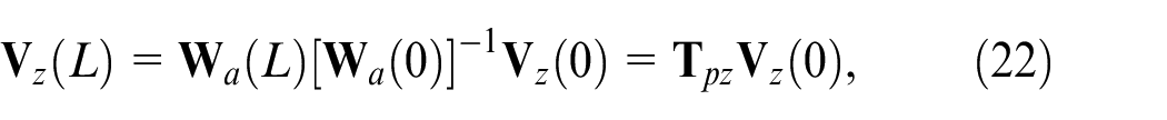
where
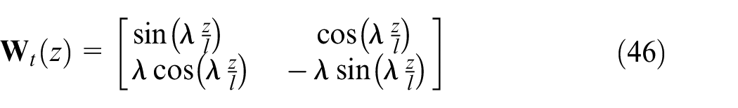
Flexural vibration impedance
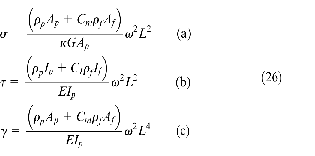
The flexural vibration governing equation of a fluid-filled straight pipe can be written as:
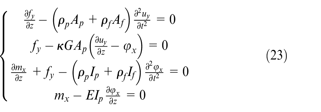
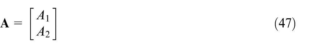
There are four unknown variables,
Substituting equation (24) into equation (23), and simplifying it to be only in terms of
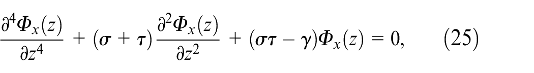
where:
It can be supposed that the solution of equation (25) has a dimensionless form, as follows:

where

The roots of equation (28) can be written as:
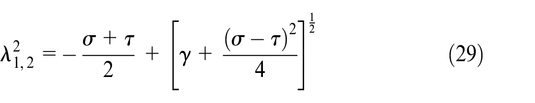
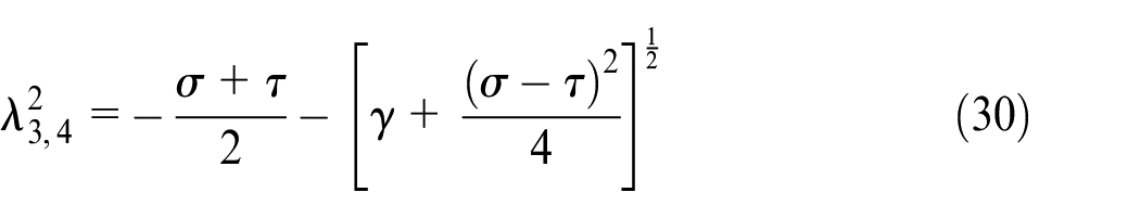
Thus, the root of equation (27) can be expanded as:
where
Substituting equation (31) into equation (23), we can obtain the exact solutions for the other three unknown variables:
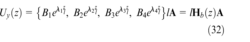
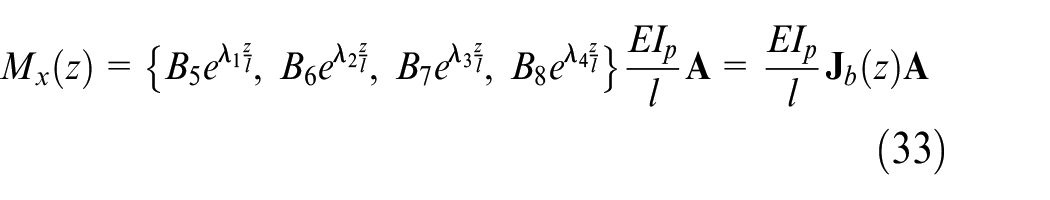
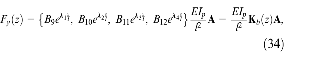
where:
Writing these in matrix form:

where:
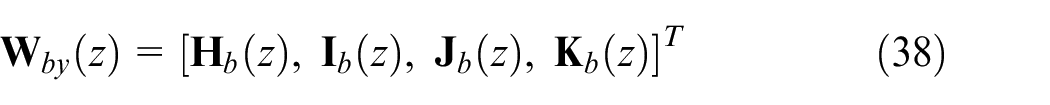
For a straight pipe with length L, according to equation (36), we can get:


Combining equations (39) and (40), and eliminating the unknown A gives:
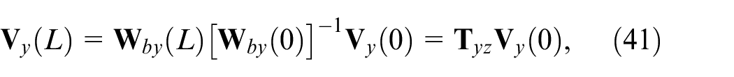
where
Torsional vibration impedance
The torsional vibration governing equation can be written as:
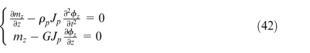
There are two unknown variables
Substituting equation (43) into equation (42), we can easily get the solution of equation (42) as follows:
where
where
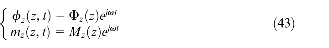
The torsional transfer matrix of a pipe with length L can be written as:

Thus, the total 14 × 14 transfer matrix of one straight fluid-filled pipe can be written as:
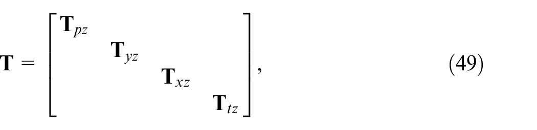
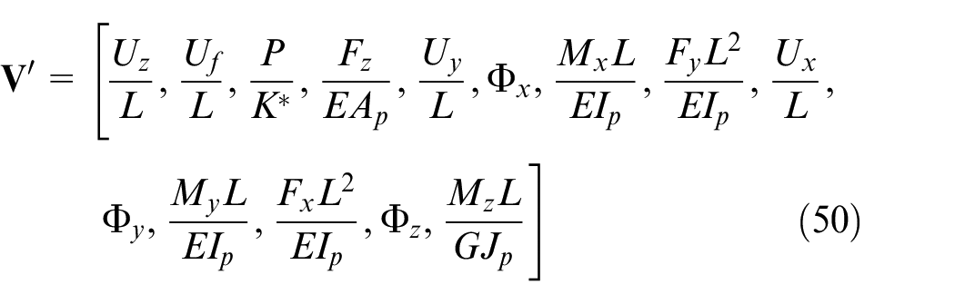
where the state vector of two ends of the transfer matrix is:
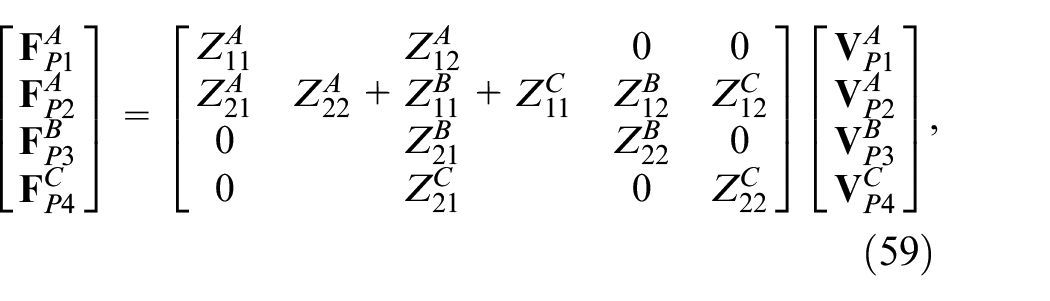
Assembly of the pipe system
Coordinate transfer
All variations of the above fluid-filled transfer matrix are based on the local coordinates of a straight pipe, as shown in Figure 1. Pipes with different directions have their own local coordinates that must be converted into global coordinates. Therefore, we transform the total 14-equation transfer matrix from local coordinates into global coordinates. The transformation matrix can be written as:
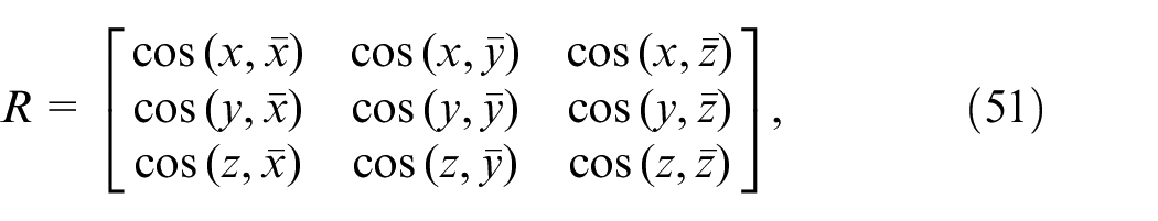
where

As the pressure and displacement of the internal fluid are always in the pipe axial direction, according to equation (52), the total coordinate transfer matrix can be written as:
The transfer matrix of a straight fluid-filled pipe in global coordinates is:
According to the relation between the transfer matrix and impedance matrix, the impedance matrix of the straight fluid-filled pipe in global coordinates can be written as:
The present method can deal with arbitrary boundary conditions and excitation. Taking flexural vibration as an example, the impedance matrix of a straight pipe can be written as:
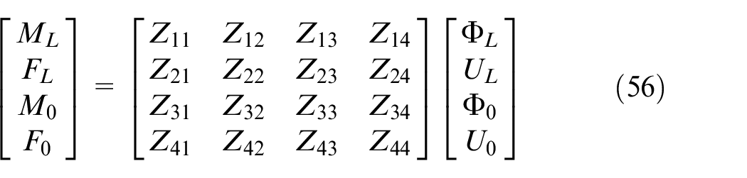
Arbitrary boundary conditions can be achieved by setting the displacement cross element in the impedance matrix to a larger number. For example, if the z = L end is fixed, which means
Other boundary conditions and excitation methods are deduced in the same way.
Impedance matrix of a branched pipe
A branch pipe is different from a straight pipe, and a strong fluid-structure interaction phenomenon will occur at the connection between the two, such as boundary and junction coupling. The typical branch pipe structure is shown in Figure 2 below and is composed of a main pipe and a branch pipe, with an angle
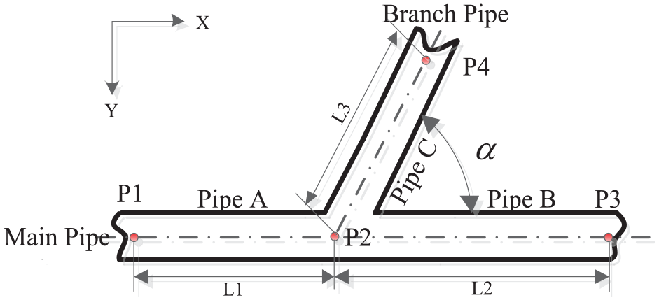
The branch pipe.
Despite the continuous displacement and force balance boundary at the connection point P2, the fluid boundary inside the pipe is very important. It should satisfy the conditions of continuous pressure and equal flow at point P2, which can be written as:
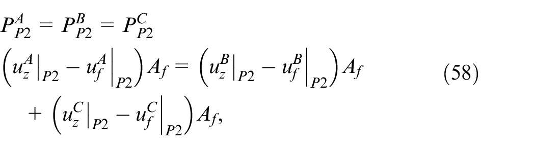
where
where:
Numerical results and discussion
The Dundee pipe
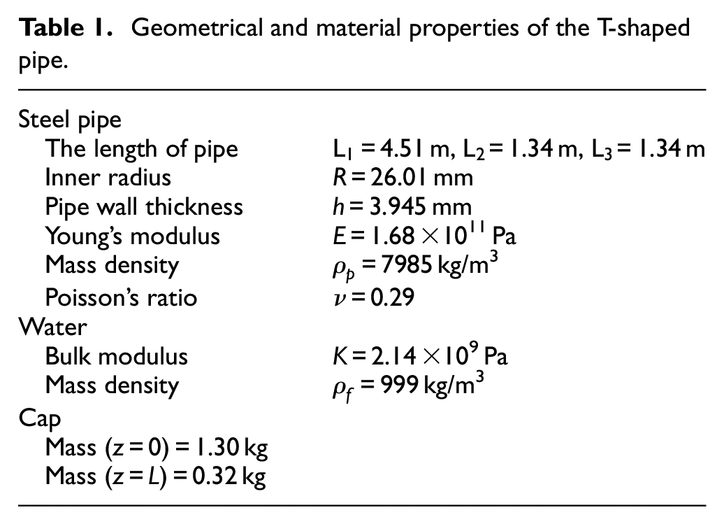
In order to verify the validity of the method proposed above, results were calculated for a Dundee branch pipe to compare with experimental data. As shown in Figure 3(a), this system is T-shaped with two branches, and equation (59) can be applied. The parameters involved in the illustration are listed in Table 1.
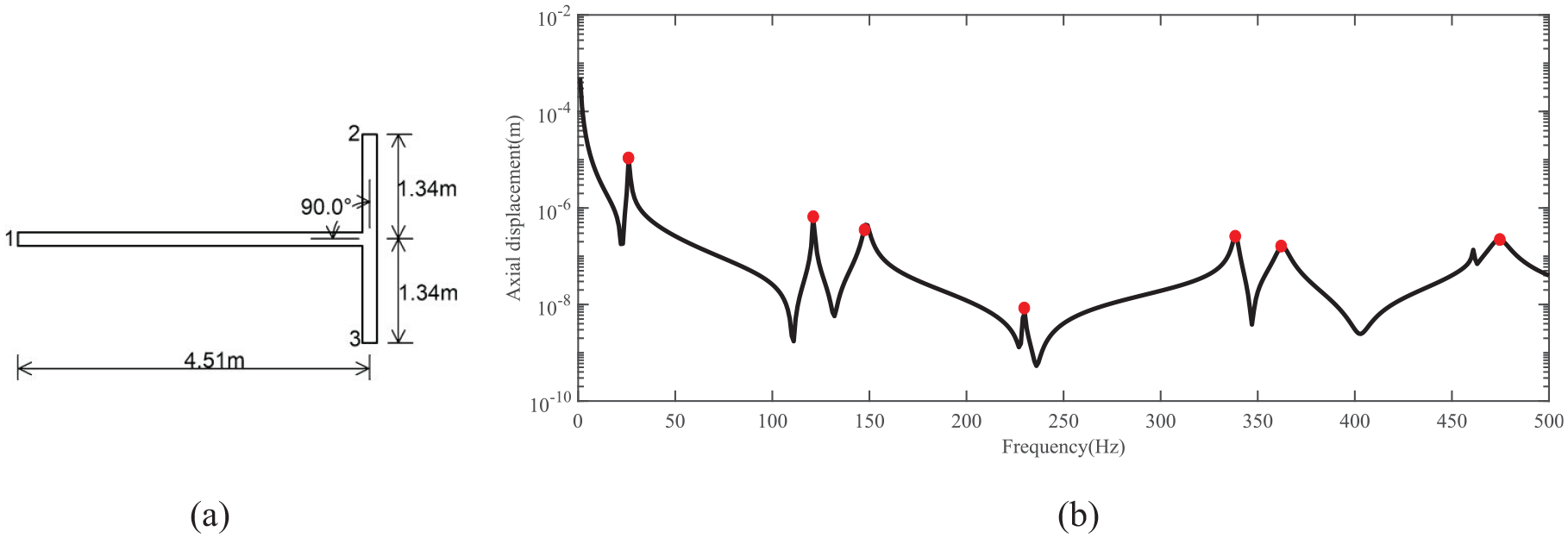
Displacements at the main pipe end: (a) geometric dimension (b) displacement.
Geometrical and material properties of the T-shaped pipe.
The frequency response of P1 is shown in Figure 3(b). There is a relation between the peak frequency of the transfer function and the natural frequency.
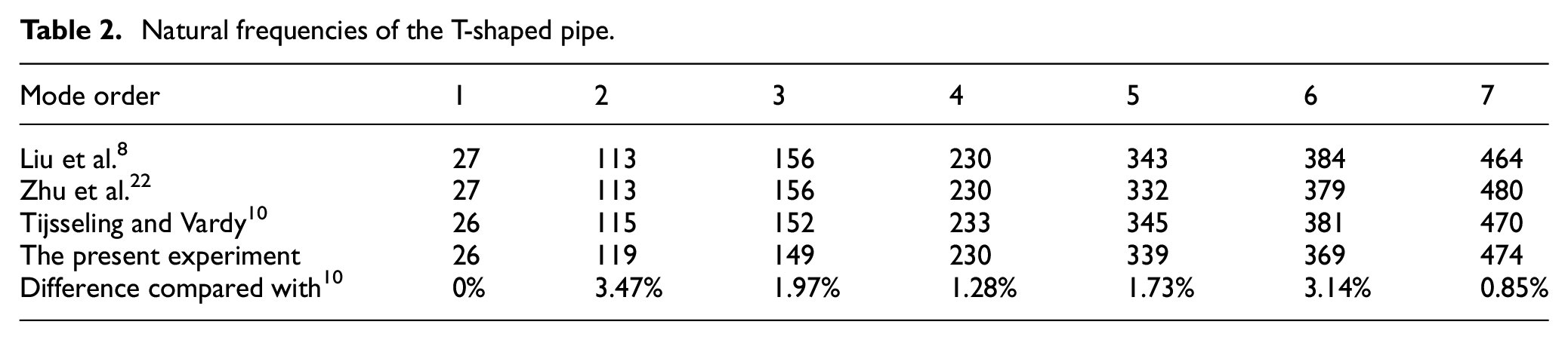
The resonance frequencies observed in Figure 3(b) are compared with the natural frequencies provided in the literature from the absorbing transfer matrix method, 8 the spectral element method, 22 and the experimental data 10 in Table 2.
Natural frequencies of the T-shaped pipe.
Comparison with the FEM model
Straight fluid-filled pipe
A straight fluid-filled FEM model is shown in Figure 4. The length of the pipe is 1.5 m, its diameter is 80 mm, and its thickness is 5 mm. The pipe is made of shell elements with a mesh size of 0.01 m. There is a total of 3725 elements in the pipe. The density, Young’s modulus, and Poisson’s ratio of the pipe are 7800 kg/m3, 2.1 ×10¹¹ Pa, and 0.3, respectively. The fluid is made up of acoustic elements and the mesh size is 0.01 m. There are a total of 11,700 elements of water. The bulk modulus and density of the fluid are 2.14 ×10⁹ Pa and 1000 kg/m3. The mass of the pipe and fluid are 14.7 and 7.54 kg.
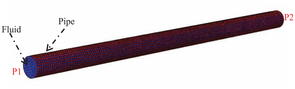
The FEM model of the fluid-filled straight pipe.
The freedom of the P2 end is fixed and the fluid inside the pipe is blocked. Excitation is applied at P1. Figure 5(a) compares the lateral displacement of point P1 under harmonic flexural excitation. Figure 5(b) shows compares the axial displacement and Figure 5(c) shows the velocity of the fluid at point P1 under a harmonic axial force. Pressure excitation is also very important in fluid-filled pipe systems, and Figure 5(d) shows the displacement of P1 compared with the FEM results under a unit harmonic pressure excitation.
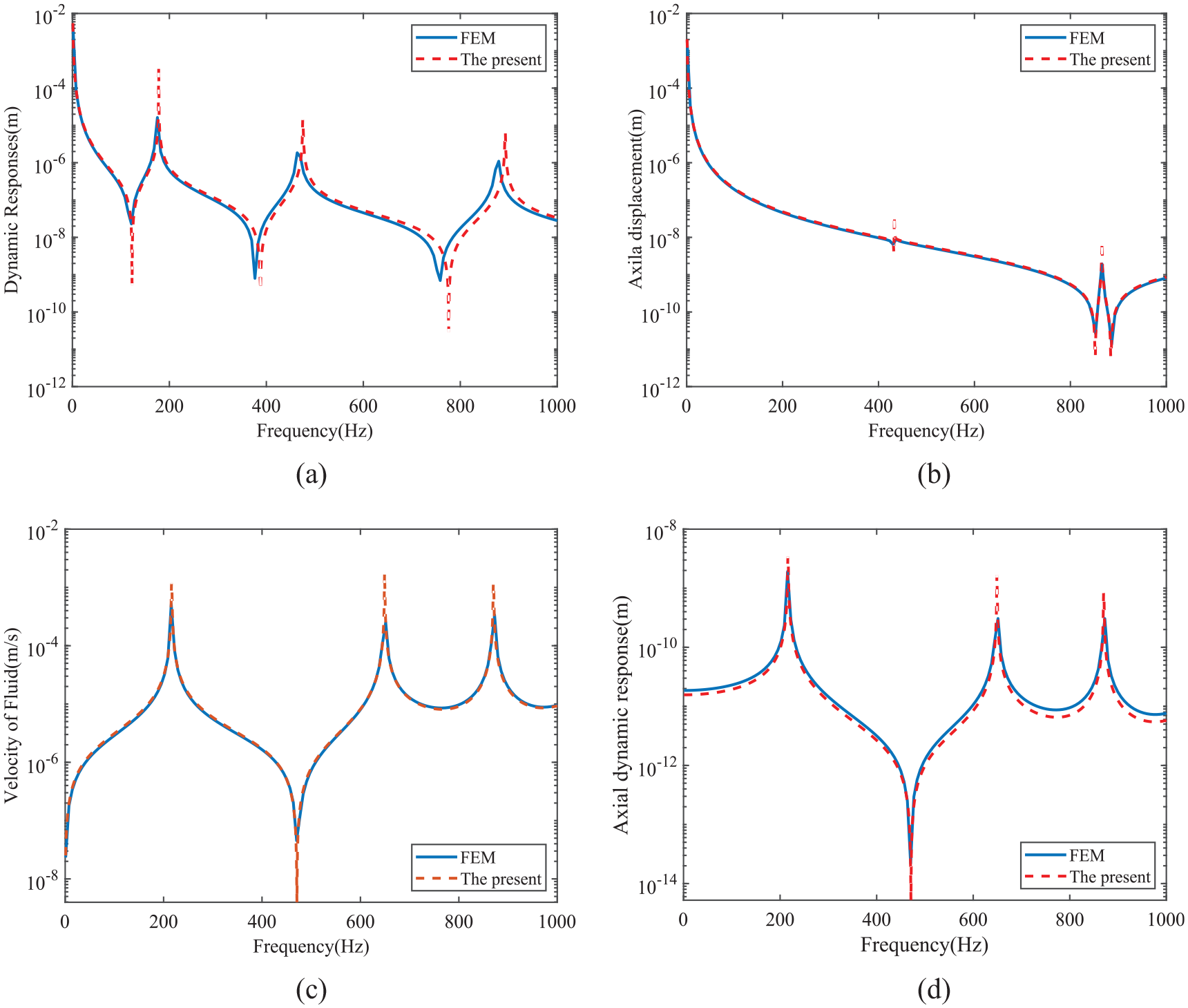
A comparison with the FEM results: (a) displacement under a flexural harmonic force, (b) displacement under an axial harmonic force, (c) velocity of the fluid under an axial harmonic force, and (d) displacement under a pressure excitation.
The four numerical cases all show that the present results are in good agreement with the FEM results, both under force or pressure excitation. The computer used for the FEM is an Intel(R) Core(TM) i7-4770 CPU @ 3.40 GHz with a memory of 16 GB. The total calculation time of the FEM model is almost 80 min, whereas the calculation time of the current analytical method is about 8 s, which makes the present method 600 times faster than the FEM.
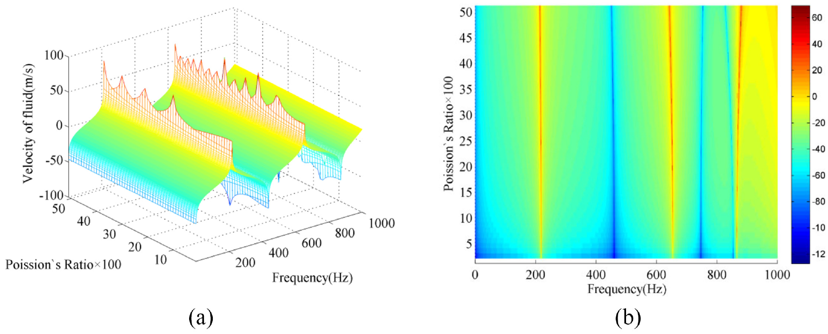
For straight fluid-filled pipes, Poisson coupling is very important.
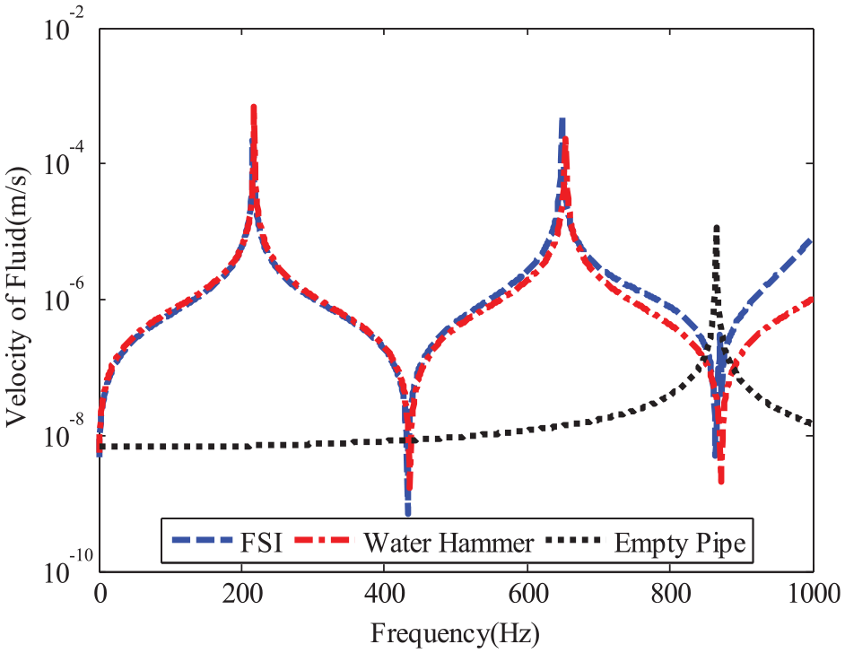
Velocity of the fluid.
Figure 7(a) shows a three-dimensional view of the effect of Poisson’s ratio on the fluid velocity and Figure 7(b) shows the top-down view. As in Figure 6, the first two peak frequencies are affected by the water hammer, so with the increase in Poisson’s ratio, these two spectral lines do not change. However, the amplitude in Figure 7(a) is obviously affected by Poisson’s ratio. Figure 7(b) shows the third spectrum moves to a high frequency with the increase in Poisson’s ratio, and the highlight becomes more obvious.
The velocity of the pipe wall: (a) 3-D view (b) Top view.
Figure 8(a) shows the effect of the fluid-to-pipe density ratio on the velocity of the fluid. Figure 8(b) shows the effect of the fluid-to-pipe density ratio on the velocity of the pipe. In both cases, the frequency spectrum moves to the low-frequency domain with an increasing density ratio. But in Figure 8(b), there remains one straight spectrum frequency, due to the vibration mode of the pipe structure itself.
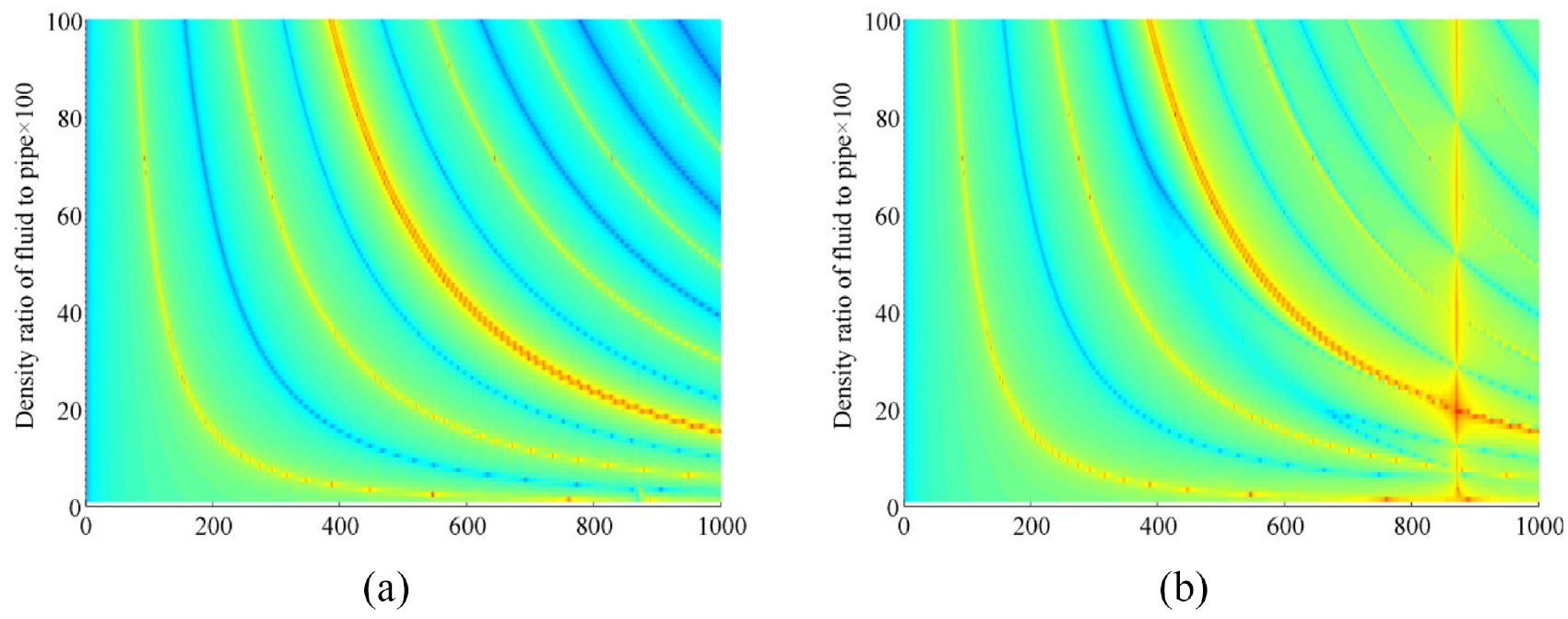
The effect of the ratio of the density between the fluid and pipe: (a) the velocity of the fluid and (b) the velocity of the pipe.
Figure 9(a) shows the effect of the thickness-to-diameter ratio on the velocity of the fluid. With increasing thickness, the peak frequency moves toward the high-frequency range, and the Poisson’s coupling becomes even less obvious. Figure 9(b) shows the effect of the ratio between the thickness and diameter on the velocity of the pipe. The moving speed of the frequency peak can be seen more obviously. The effect on the peak frequency movement is more obvious for a low ratio. With an increasing ratio in the high-frequency range, the highlight remains an unchanged line.
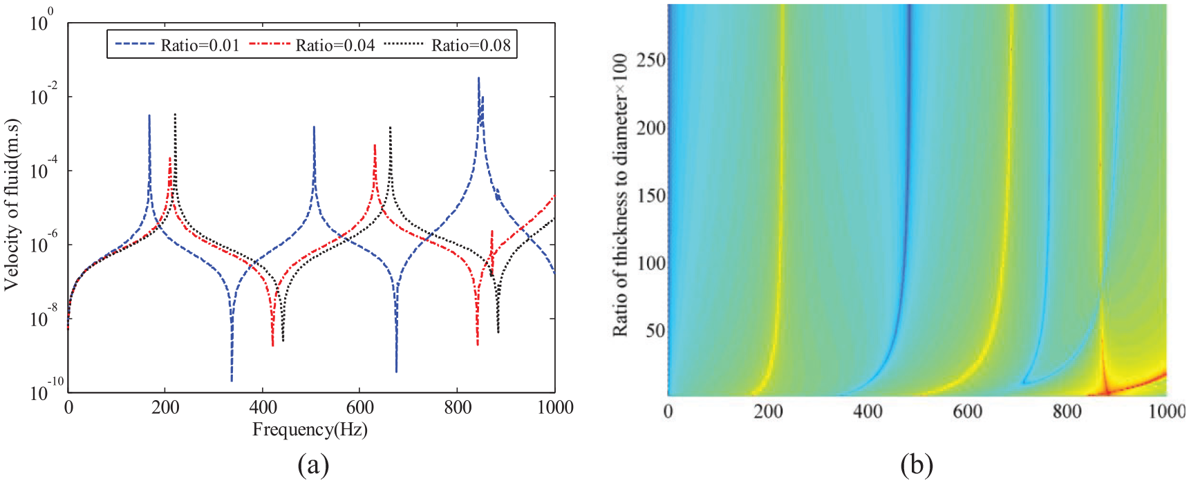
The effect of the ratio of the thickness to diameter: (a) the velocity of the fluid and (b) the velocity of the pipe.
Compared with the finite element method, the calculation method in this paper has a wide frequency range and fast calculation time. It can provide a fast, stable, and convenient tool for the vibrational parameter analysis of a pipe system, as shown in Figures 7 to 9.
Branch pipe
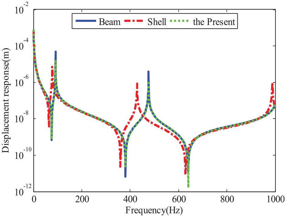
The validation for a branch pipe is presented in this section. A unit harmonic excitation is applied at Node 1 in the X direction. The length of the main pipe is 2.0 m and the length of the two branch pipes is 1.0 m. There are two kinds of finite element models for T-type pipes; one is made of beam elements and the other is made of shell elements, as shown in Figure 10. Both mesh sizes of the beam and shell model are 0.01 m, and there are a total of 400 beam elements and 10,797 shell elements. The grid size is selected according to the upper limit of the calculated frequency, and the corresponding wavelength should contain six elements. The outer radius and thickness of the pipe are 80 and 5 mm. The Young’s modulus and Poisson’s ratio are E = 210 × 109 Pa,
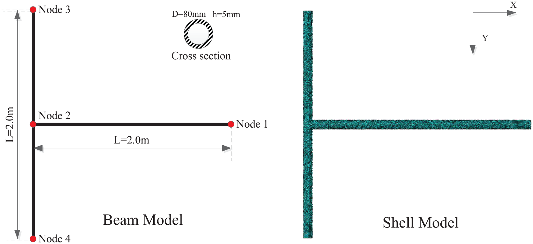
The FEM model of the branch pipe.
The dynamic displacements of Node 1 in the X direction are compared in Figure 11. The three results overlap in the low-frequency domain, but with increasing frequency, the FEM shell element calculation result becomes different from the other two results. The FEM beam element result is almost the same as the present result over the whole 1000 Hz frequency domain. The discrepancy seen for the shell model is due to the existence of higher-order circumferential modes in the shell model, and because the finite element method cannot simulate the effects of connection coupling. This is why there is almost no literature validating the FSI of a branch pipe using the FEM method. The disadvantage of the present method is that the theoretical part is based on the beam model, and it is correct in the cut-off frequency range of the pipe but is no longer applicable in the high-frequency range. In addition, the number of grid points and the calculation cost of the shell model are far greater than those of the beam model, but the beam model in FEM cannot simulate Poisson coupling. Therefore, the analytical method based on the beam model in engineering predictions meets practical engineering requirements.
The dynamic displacement of the branch pipe.
Over the entire frequency domain, there exist two frequency peaks at 92 and 476 Hz, but three frequency peaks are seen for the shell element method. The peak frequencies are related to the natural frequencies of the model, so the six in-plane vibration modes are plotted in Figure 12. It can be seen that the vibration mode of the two branches is the main reason for the peak frequency in the axial displacement.
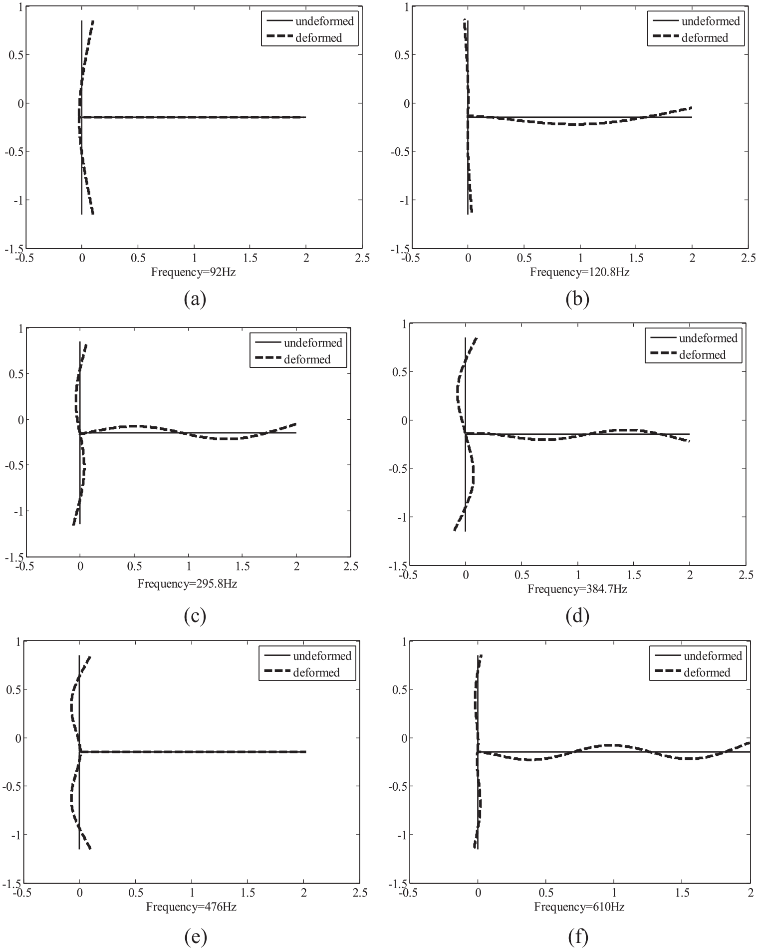
The first six in-plane vibration modes of the T-type branch: (a) 1st mode, (b) 2nd mode, (c) 3rd mode, (d) 4th mode, (e) 5th mode and (f) 6th mode.
Unlike a straight fluid-filled pipe, in this case there is not only Poisson coupling, but also strong junction coupling at the branch pipe due to the discontinuity in geometry. Figure 13 shows the effect of the angle of the branch pipe on the axial displacement at Node 1.
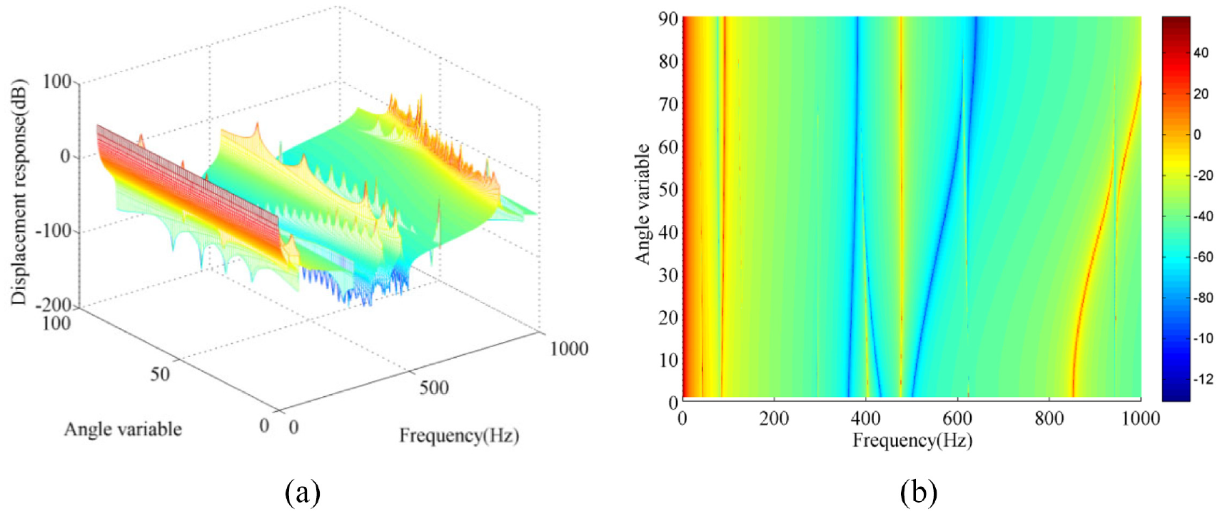
The effect of the angle of the branch pipe: (a) 3-D view and (b) Top view.
Figure 13(a) shows the origin three-view, where the x-axis indicates the frequency, the y-axis represents the angle of the branch pipe, and the z-axis is the axial displacement at Node 1 (dB, ref: 10–6 m). The figure shows that the angle of the branch pipe can change the amplitude and frequency of the displacement. Figure 13(b) shows the top-down view and it can easily be seen that both the peak and trough frequencies are changed by the angle, although some remain unchanged.
Experimental data
Flexural vibration of a straight pipe
An experiment on a simple straight steel pipe is carried out to verify the calculation method in this paper. The straight steel pipe is excited by a horizontal electric shaker at the top end and the lower end is fixed by an infinite rigid clamp, as shown in Figure 14. As boundary conditions, one end is free while the other end is fixed (structure) and blocked (fluid). The length, radius, and thickness of the pipe are 1.0 m, 40 mm, and 5 mm, respectively. The total mass of the pipe is about 16 kg. There are three acceleration sensors and one force sensor installed on the pipe. The signal generator produces 10–2000 Hz frequency range white noise, which is enlarged by a power amplifier.
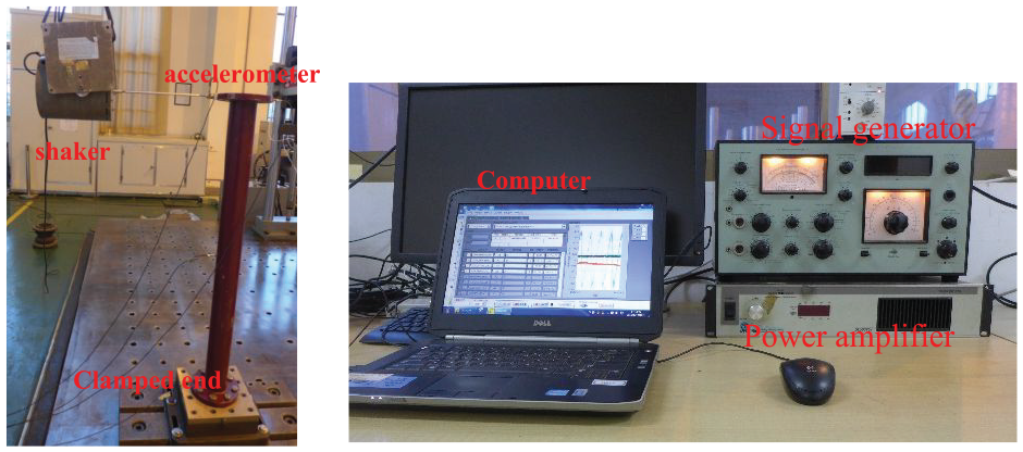
Experimental straight pipe device.
There are two cases considered in the experiment. The first is a pipe without water and the second is a pipe filled with water. The frequency responses calculated by the impedance synthesis method are compared with those of the test in Figure 15. It is easy to see that the two results are close to each other. Due to the mass added by the internal fluid, the second vibrational peak frequency is moved to lower regions. Because there are no bend pipes or branch pipes, the interaction between the pipe wall and the fluid is weak.
A comparison of the numerical and experimental results for a straight pipe: (a) without water and (b) with water.
Space fluid-filled pipe
In addition, a complex three-dimensional fluid-filled pipe system is proposed to verify the present method. The experimental pipe system consists of seven straight pipes, two bends, and two T-type branch pipes, as shown in Figure 16. All of the pipes can be classified into five geometric sizes (A, B, C, D, and E), as shown in Figure 16. Flanges are also installed at both ends of the pipeline.
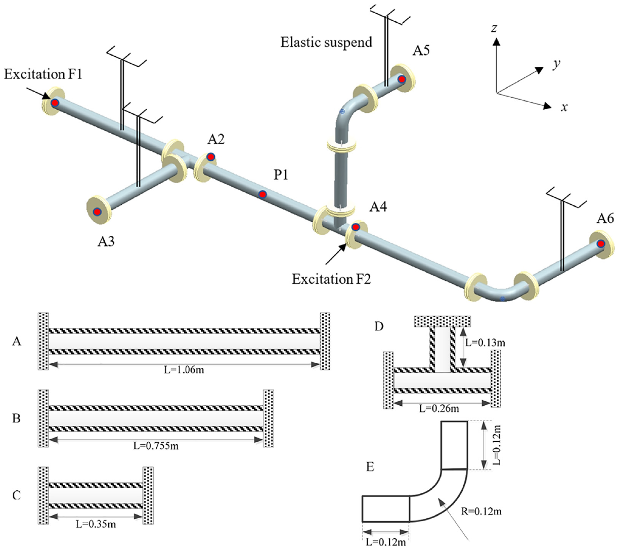
The experimental space pipe system.
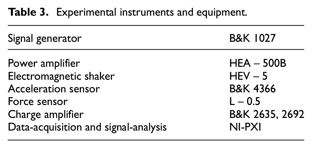
The diameters and thicknesses of all pipes are 89 ×4.5 mm, and the whole system is filled with water. The instruments and equipment used in the test are listed in Table 3. The ends of the pipes are blocked by flanges. The whole pipe system is suspended by four elastic ropes, as shown in Figure 17. The boundary for the pipe is free, and that for the fluid is blocked.
Experimental instruments and equipment.
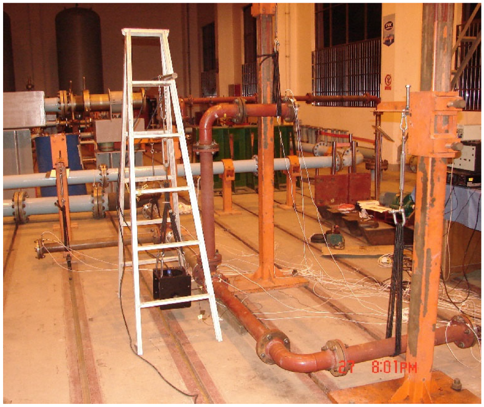
A photo of the elastic-suspended space fluid-filled pipe.
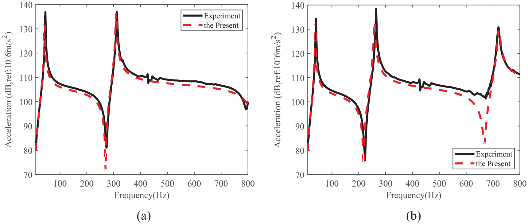
Two excitation cases are considered. One involves an excitation at point A1 in the X direction and the other an excitation at point A2 in the Y direction. Figure 18(a) compares the experimental and numerical results of point A1 in the X direction, and Figure 18(b) compares the experimental and numerical results of point A5 in the Y direction in Case 1.
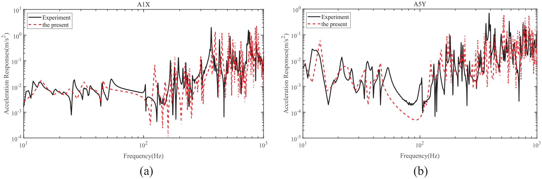
A comparison of the calculation results with experimental data under excitation in the X direction: (a) point A1 in the X direction and (b) point A5 in the Y direction.
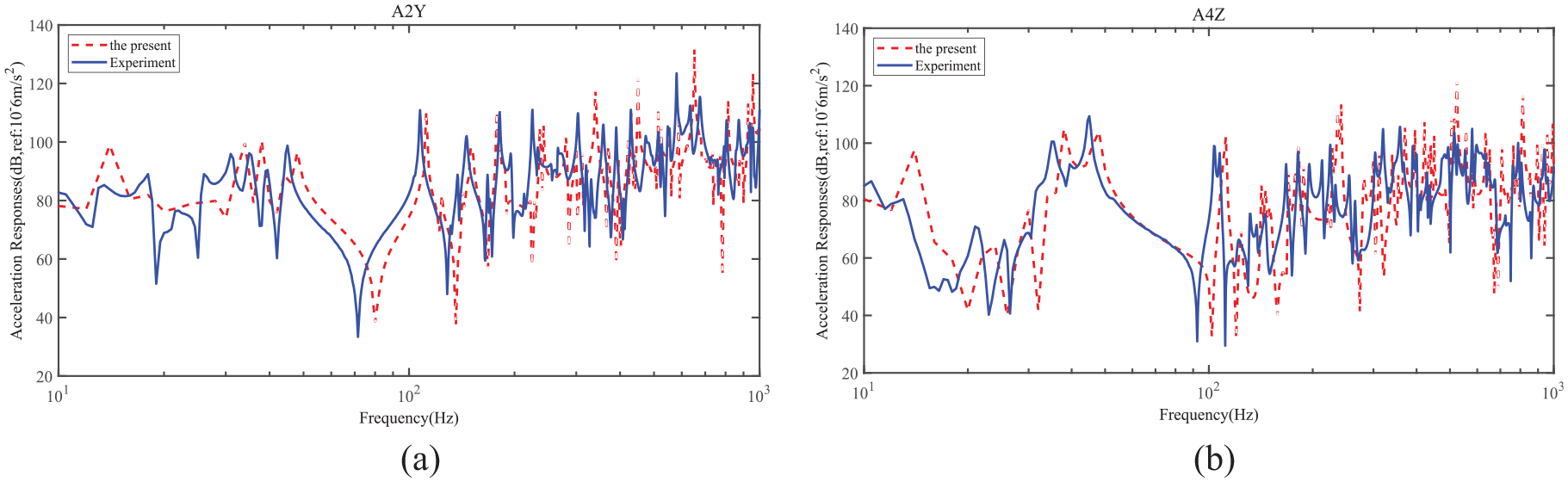
Figure 19(a) shows a comparison of the experimental and numerical results at point A2 in the Y direction, and Figure 19(b) shows a comparison of the experimental and numerical results of point A4 in the Z direction in Case 2.
A comparison of the calculation results with experimental data under excitation in the Y direction: (a) point A2 in the Y direction and (b) point A4 in the Z direction.
It can be seen from the figures that the calculation results in this paper are basically consistent with the experimental results in the range around 1000 Hz, which validates the accuracy of the calculation method in this paper.
Conclusions
A method for analyzing dynamic responses using the impedance synthesis approach has been developed, which is suitable for a three-dimensional fluid-filled pipeline system. Two different models were established to ensure the validity and accuracy of the new method. The results of a simple T-shaped pipe were combined with data given from FEM and in the literature, and a more complex spatial pipe system was examined to measure the excitation data from a shaker. The following conclusions can be drawn:
The impedance synthesis method is a suitable, correct, and effective method for FSI analysis of a three-dimensional fluid-filled pipe, and could be used to provide valuable suggestions for pipe vibration control and design.
The in-plane vibration mode is the main reason for the dynamic peak frequency of a T-shaped fluid-filled pipe.
The peak FSI frequency in a fluid-filled pipe is affected by both a water hammer and an empty pipe.
Footnotes
Declaration of conflicting interests
The author(s) declared no potential conflicts of interest with respect to the research, authorship, and/or publication of this article.
Funding
The author(s) disclosed receipt of the following financial support for the research, authorship, and/or publication of this article: This work was supported by Foundation of National Key Laboratory on Ship Vibration & Noise under Grant number JCKY2019207CI02, People’s Republic of China. The authors also gratefully acknowledge financial support from China Scholarship Council (202008320401).
Data availability statement
The data that support the findings of this study are available from the corresponding author upon reasonable request.