
Abstract
To achieve a fully autonomous navigation for unmanned surface vessels (USVs), a robust control capability is essential. The control of USVs in complex maritime environments is rather challenging as numerous system uncertainties and environmental influences affect the control performance. This paper therefore investigates the trajectory tracking control problem for USVs with motion constraints and environmental disturbances. Two different controllers are proposed to achieve the task. The first approach is mainly based on the backstepping technique augmented by a virtual system to compensate for the disturbance and an auxiliary system to bound the input in the saturation limit. The second control scheme is mainly based on the normalisation technique, with which the bound of the input can be limited in the constraints by tuning the control parameters. The stability of the two control schemes is demonstrated by the Lyapunov theory. Finally, simulations are conducted to verify the effectiveness of the proposed controllers. The introduced solutions enable USVs to follow complex trajectories in an adverse environment with varying ocean currents.
Keywords
Introduction
The term unmanned surface vessels (USVs) refers to marine vehicles that can achieve the required operation on the water surface autonomously. 1 USVs can be widely used for various applications in the maritime sector, including transportation, environmental investigation, resources exploration and military operations. 2 Since USVs do not require any human intervention, the deployment of USVs can potentially increase personal safety, operational range and precision and flexibility in a harsh environment. 3 Therefore, the research and development of USVs have become a significant part of marine robotics with substantial effort contributed by many researchers and engineers in recent decades. 4 In particular, the increasing reliance on the ocean has stimulated a growing demand for the development of USVs.
To ensure safe navigation of USVs, an autonomous navigation system (ANS) is the most critical part. In general, an ANS consists of three essential capabilities, including sensing/perception, planning and control. Among them, the control module directly operates on autopilot and propels USVs to robustly follow the defined trajectories. Consequently, the design of a robust controller for USVs is of pivotal importance and is associated with challenges such as systems nonlinearity and uncertainties, underactuation of vessels dynamics, control input saturation, external disturbances, etc. 5 These problems leave challenges to the researchers and demonstrate the need for further development for USVs.
In essence, the development of control strategies is oriented by different control objectives, including: (1) set point control, (2) path following control and (3) trajectory tracking control. 3 Setpoint control forces the position and heading of the ship to the desired value without time requirement. It is the most basic control objective and plays an important role in dynamic position for fixed target operation such as autonomous docking. 6 However, setpoint control cannot be achieved using continuous control inputs. 3 Therefore, it is only used in some special missions and does not attract much interest from researchers.
Path following control requires a USV to follow a specified path with a certain speed without temporal constraint. 7 It can be achieved by using a continuous controller and has less stringent control requirements than trajectory control. The most popular approach to achieve the path following control is by using the Lookahead-based line-of-sight (LOS) guidance law. 5 The basic idea is to mimic the performance of a helmsman, setting the course angle based on the ratio of the cross-track error and look ahead distance. 8 Based on the LOS guidance law, Zheng and Sun 9 proposed using a backstepping technique augmented by radial basis function neural network (RBFNN) and an auxiliary design system to achieves the path following control. A finite-time currents observer based ILOS guidance law combined with the adaptive technique are used in Fan et al. 7 to address the path following control.
Different from the path following control, of which the path has no temporal constraint, trajectory tracking control requires a USV to track a trajectory with spatial and temporal constraints. 10 Therefore, it is more general and compatible to handle more complicated missions. Thus, as the complexity of the missions has increased, further development for trajectory control is required. The trajectory tracking control of USVs can be mainly divided into control of the fully actuated ship and control of the underactuated ship, 3 with the former being already reasonably understood, whereas the understanding of the latter still limited.
More specifically, USVs with common configurations have only two controls, that is the surge force and yaw moment, while the sway axis is not actuated. Thus, the motion of three degrees of freedom will be controlled by only two inputs, which makes it a typical underactuation problem. 9 Several control methods have been attempted to realise the trajectory tracking for underactuated USV, including the backstepping technique, 11 sliding mode control, 12 model predictive control, 13 dynamic surface control, 14 linear algebra-based approach, 15 and intelligent control strategies. 16 The most popular methods are the backstepping technique, which is usually combined with Lyapunov’s direct method, and sliding mode control that characterises the tracking error through the use of the sliding surface. As the sliding mode can suffer from chattering effects and imposes high loads on the actuator, the backstepping technique is used more in the trajectory tracking problem. 5 The basic idea behind the backstepping technique is to treat some of the states as ‘virtual controls’, and then design the virtual control laws as the control through Lyapunov’s direct method. 9 Pettersen and Egeland 17 firstly proved that a USV system was controllable and raised a potential control law. However, only exponential stability was obtained. Dong et al. 18 used a controller based on modified backstepping technique and enriched by integral action and achieved the trajectory tracking control with better steady and transient performance.
The above-mentioned control scheme for trajectory tracking control does not take the motion constraints into consideration. Therefore, the desired actuator’s output and the vehicle’s velocity can be infinite, so that input saturation is required. The ignorance of the input saturation will lead to performance degradation, lag, overshoot, as well as instability in the closed-loop response of practical systems. 9 For this reason, it is of great theoretical and practical significance to design a control scheme to handle motion constraints. The motion constraints mainly include the constraints of the yaw torque and surge velocity. A Gaussian error function has been used to approximate the input saturation of the actuators and globally uniform ultimate boundness of the system was achieved. Wang and Zhang 19 designed an auxiliary design system to handle input saturation through adaptive control. However, these studies mostly focus on the saturation limit of the actuator, while the constraints of the velocity are always ignored. Therefore, these controllers must be developed by taking the velocity constraints into consideration.
Apart from the input saturation, another vital factor that is ignored in many studies is the external disturbance caused by the ocean current. Without the consideration of the environmental disturbance, a ship will deviate from the desired trajectory. Chen 20 proposed that, for a general control system with disturbance, the disturbance can be cancelled by setting the control input to be linearly dependent on the disturbance. However, this method cannot be directly used for realising the trajectory tracking of USVs due to their underactuated nature. Fossen and Lekkas 21 used the sign function inside the controller to handle the disturbance. However, this method may make the system chatter and introduced discontinuous control variables. Zhu and Du 22 used an adaptive estimate law and a finite-time disturbance observer to handle the external disturbances. Qiu et al. 23 proposed a sliding mode surface control scheme cooperated with adaptive technology to deal with the external disturbance. These control methods mainly used adaptive estimation law, mostly cooperated with disturbance observer, to estimate and compensate for the unknown ocean currents, which suits for situations that the ocean currents are hard to be measured.
The ocean current velocity can be measured in real time with acoustic doppler profilers installed on the bottom of the vessel integrated with global positioning systems.24,25 Thus, it is possible to design a control scheme based on known ocean current information. In the current literature of trajectory tracking control for unmanned systems, some controllers are designed based on the kinematic model only,26,27 and some also incorporate the full dynamic model.19,22 The advantage of the controller based on the kinematic model is that it can be easily applied in commercial unmanned vehicles cooperated with a well-developed propulsion system, which only requires the velocity signals to control the ship. 28 In addition, control algorithms based on the kinematic model can be easily extended into the control of multiple USVs, 29 as most current research on coordination control is based on the kinematic model due to the complexity of the system. 30 As the focus of this study is on the constraints and influence of external disturbances on the velocity, considering only the kinematic model is more suitable for this problem, while the control of the dynamic systems can be easily achieved independently through the backstepping technique. Thus, it is possible to design a control scheme based on known ocean current information. Motivated by the above reasons, this paper develops two robust control schemes to achieve the trajectory tracking control for the USV under motion constraints with and without considering external disturbances. The effectiveness of both control schemes is verified through numerical simulations. The contribution of the study can be summarised as follow:
The external disturbance is considered in this study and a virtual system is introduced to handle it. It is proved that using the virtual system, the model of the USV can be simplified and the derived velocity can compensate for the ocean current.
Based on the virtual system, the backstepping technology combined with the Lyapunov direct method are used to calculate the desired control law. It is proved that the control scheme demonstrates excellent performance to achieve the trajectory tracking control of the USV with normal ability to handle the input saturation in complicated environments.
In order to improve the ability to handle the input saturation, a controller based on the normalisation technique is used to normalise the tracking error and thereby to make the velocity be related to the design parameters and reference trajectories, which can produce smoother input compliant with the practical limitation.
By using the virtual system, the complicated environmental disturbance can be solved by a simple method that has excellent performance.
The rest of the paper is organised as follow. Section 2 introduces the problem formulation, including the model of the USV and the transformation to the virtual. Section 3 presents the design of the control law. Section 4 presents the simulation results of the proposed approaches and the discussion of the result. Then the conclusion of this study and the future work are presented in section 5.
Problem formulation
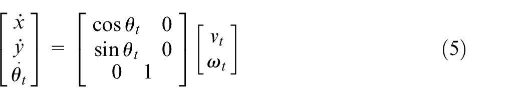
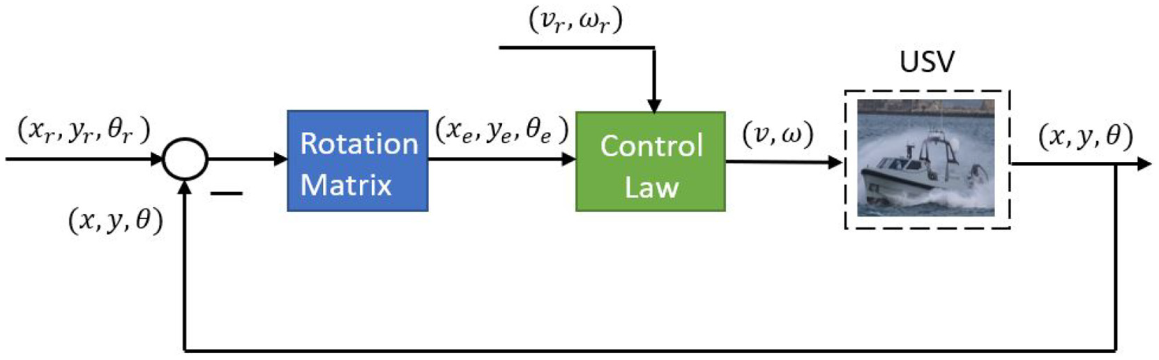
The motion of a marine surface vessel is shown in Figure 1. It is described based on two different orthogonal coordinates: the inertial and body-fixed reference frames. The inertial coordinate is fixed to the earth, with the origin located at a fixed point, the x-axis pointing to the north and the y-axis pointing to the east. The body-fixed reference frame is fixed to the ship. The USV is assumed to be symmetrical with zero trim, and the origin of the attached body-fixed frame is set to match the centre of gravity, which is satisfied for most commercial surface vessels.23,31 The x-axis points to the heading of the ship and the y-axis is perpendicular to the x-axis. The USV model in the presence of disturbance can be written as 7
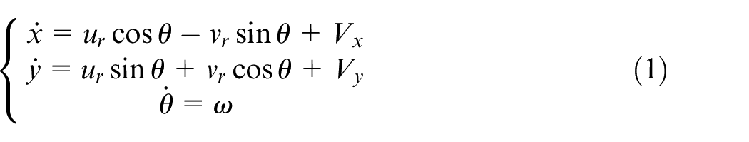
where
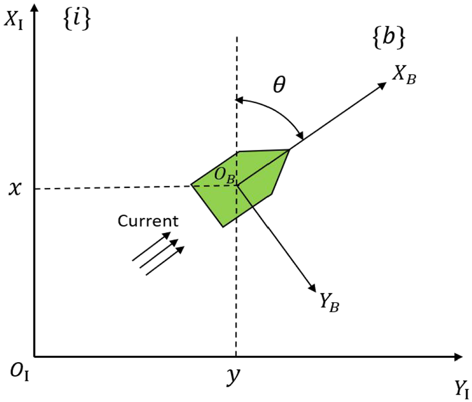
Motion of a USV.
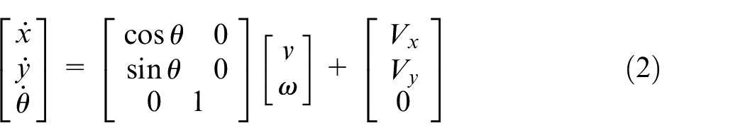
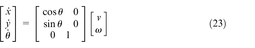
The velocity in the sway axis is small and can readily converge to zero through the control of the dynamics. Hence, it can be neglected when calculating the desired linear velocity and yaw rate.
Thus, the motion of the USV can be simplified as follows
Assumption I. The environmental disturbances considered in this study are irrotational, time-varying and bounded.
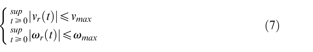
Due to the practical limitation, the velocity cannot exceed the capacity of the engine. Therefore, there exist limits for the input velocity, which can be expressed as
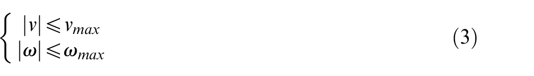
where
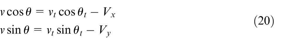
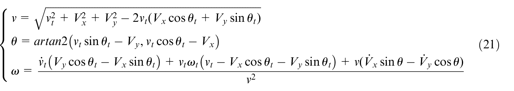
In the model of the USV, if the disturbance can be cancelled out, the derivatives of the states will become the function of only the states and inputs. Then the complexity of the system will be reduced, and the problem can be solved by using the same method as the model without the disturbance. Based on this observation and inspired by the idea of cancelling the disturbance through setting the input as a function of disturbance, virtual inputs and heading angle are introduced, which satisfy the following condition
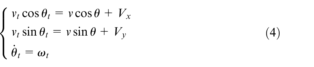
where
The reference to be tracked is assumed to be
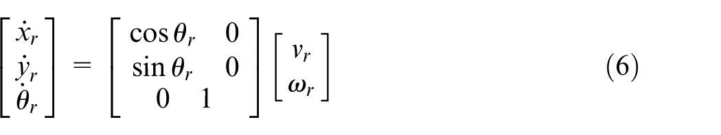
Assumption II. The reference linear and angular velocities are bounded and smaller than the limitation of the USV velocity.
Remark II. This assumption is practical, as the reference velocity cannot exceed the capacity of the engine. Otherwise, the ship can never achieve the tracking assignment.
Then the tracking error, which is the difference between the trajectory and the USV in the body-fixed frame, can be expressed as
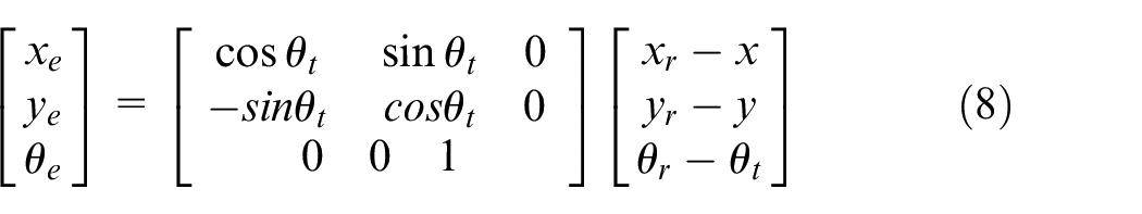
where
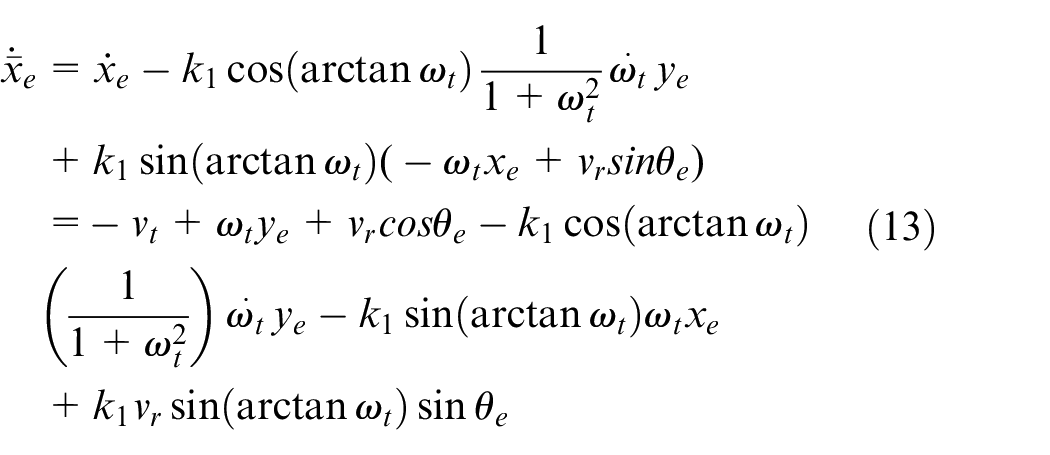
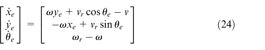
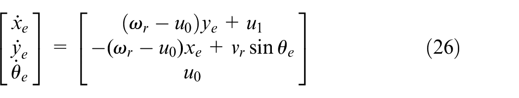
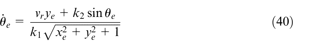
According to (5), (6) and (8), the error dynamics, which are the derivatives of the tracking error of the system, can be expressed as
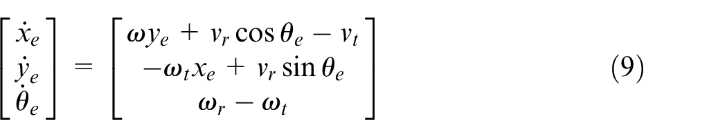
The control objective now is to find the suitable control input
The dynamic model is not considered in the design of the controller, but it could be used to verify the effectiveness of the proposed controller in the future. The dynamic model of the USV is 7
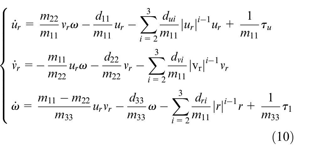
where
The proposed controller will output the desired surge velocity and yaw rate, which could be used to calculate the relative sway velocity based on equation (10). Then required torque to force the sway, surge velocity and the yaw rate to the desired value could be readily obtained through backstepping technology.
Control law design
In this section, two different trajectory tracking control schemes for USVs will be proposed. For the first controller, based on the virtual system, the backstepping technique and Lyapunov’s direct method will be used to calculate the required control law, which will finally be limited by the auxiliary system to handle the input saturation. The second controller will use the normalisation technique to make the inputs relate to the reference trajectory and design parameters only. Then, the input will be limited to the saturation limit by tuning of the design parameters.
Control law based on the backstepping technique
The first control scheme is mainly designed based on the backstepping technique and Lyapunov’s direct method. At first, to solve the undersaturation problem, the backstepping technique is used, which treats two tracking errors as virtual control inputs to stabilise the other states and design the intermediate control laws that depend on the dynamics state. Then, based on that, Lyapunov’s direct method is used to find the desired control law that stabilises the tracking error to 0.
A common USV only has control in the surge and yaw degrees of freedom, while sway is not actuated. Therefore,

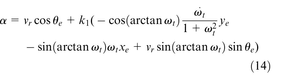
The virtual control is assumed as
In the domain of the system,
ϕ(0) = 0.
zϕ(z) > 0.
ϕ is bounded.
Examples of

Then the
A new variable
Then

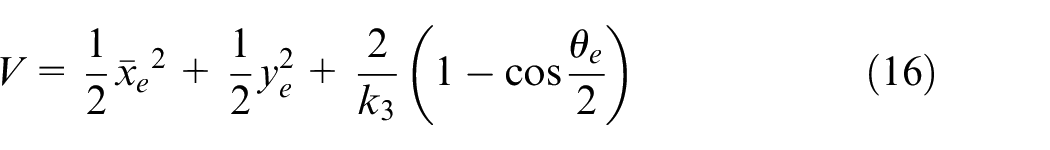
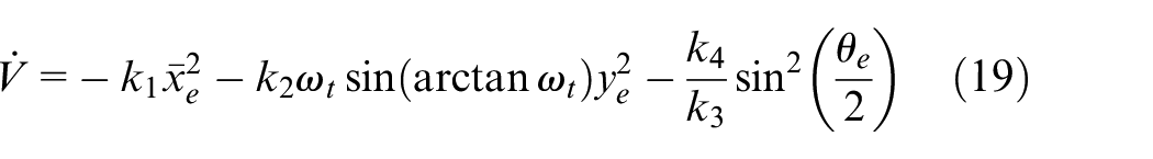
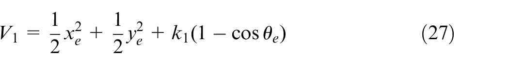
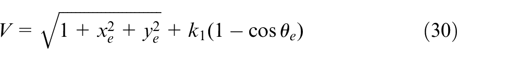
After the intermediate control law is defined, the next step is to find the desired control law through Lyapunov’s direct method. Consider the candidate Lyapunov function
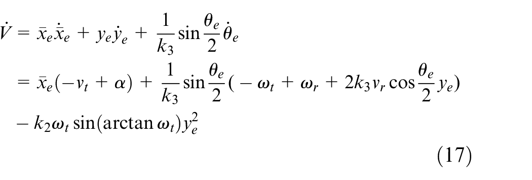
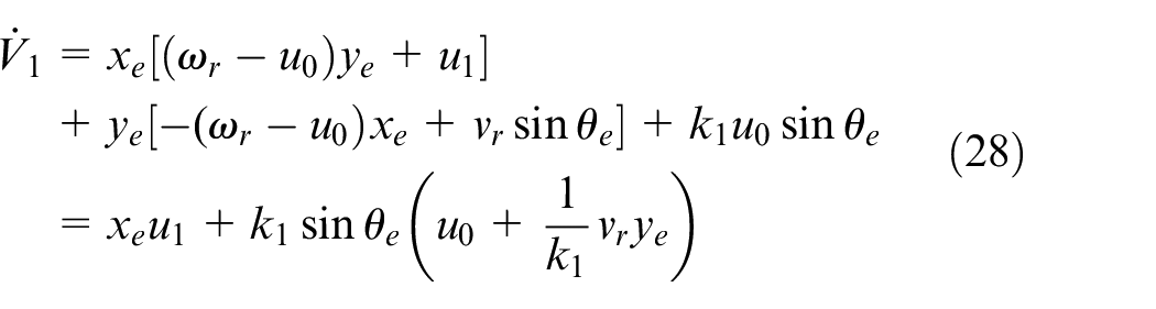
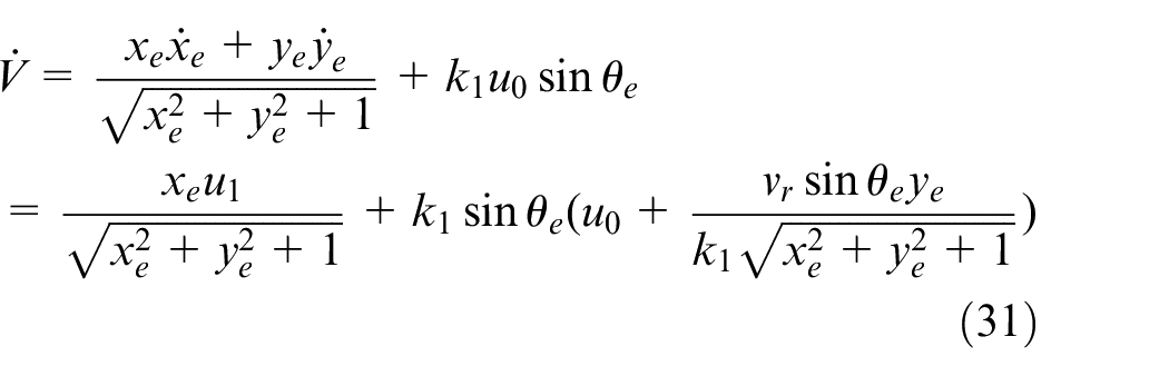
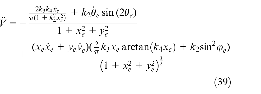
Then, the derivative of the V yields
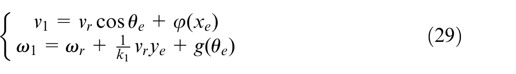
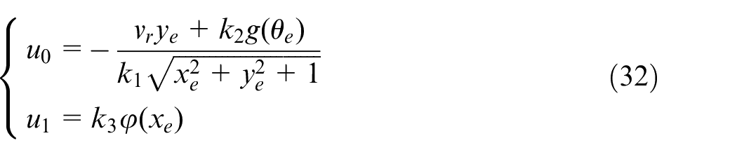
According to the property of the function that
where k2, k3 and k4 are positive design parameters.
The stability of the system with the proposed controller can be proved as follow.
Proposition 1. If
Proof At first, for the convenience of expression, the Barablat lemma is introduced.
Lemma 1. (Barbalat lemma)
If
The Lyapunov scalar function contains all the control states that can reflect the stability of the control and is positive definite.
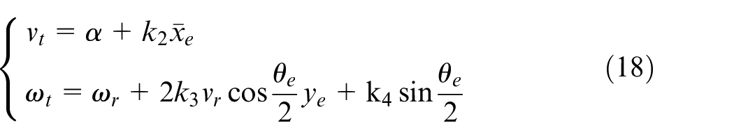
Substituting (18) into (16) yields,
As
V is differentiable and bounded and
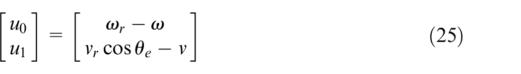
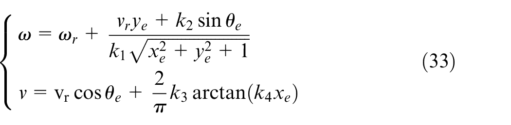
After deriving the virtual control law, the next step is to obtain the actual control input.
According to (4), the real control input satisfies the following condition,
Then by rearranging (20)
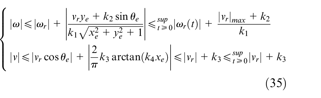
The above system may induce velocity beyond the limitation. The following auxiliary system is used to handle input saturation. Taking the input saturation of the linear and angular velocity into consideration, the final input generated by the ships are
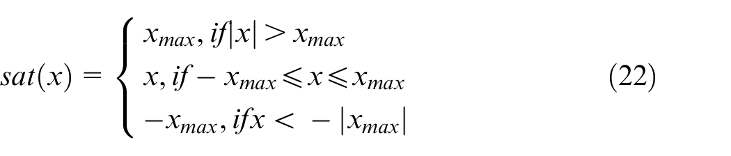
where x representing v and
The full control block for the control scheme based on the backstepping technique augmented by the virtual system and auxiliary system are shown in Figure 2.
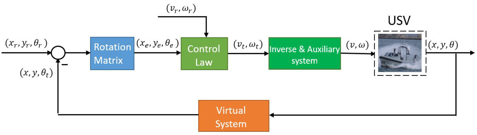
Block diagram for the closed-loop system based on the backstepping technique.
The designed controller can stabilise the error, and the performance, such as the response time and the smoothness of the control input, can be adjusted by changing the control parameters. The problem of the above designed controller is that the resulting linear and angular velocity may change sharply when it reaches the upper and lower bounds. Thus, the next method based on normalisation is proposed. The maximum and minimum velocity derived in the next controller can be set in a fixed range by changing the control parameter. Therefore, by setting the maximum and minimum velocity within the physical limitations, the sharp change of the inputs will not occur, thus resulting in better performance of the system. However, due to the uniqueness of the design, the second method is not able to handle the external disturbance. In the next section, the detail of the second method will be introduced.
Control law based on the normalisation technique
The basic idea of the normalisation technique is to normalise certain tracking errors appropriately to make the designed velocity bounded by design parameters and the reference velocity only. The controller does not take the disturbance into consideration, as the virtual system used in the last method cannot be normalised. Thus, the model of the USV without disturbance is used in this method, which is
The error dynamics based on the above system are
To further simplify the error dynamics, the new control input is defined, which is
Then error dynamics are changed to
To find the errors that need to be normalised, let us first consider a candidate Lyapunov function like the one used in the first method, which is
where
Taking the time derivative of the scalar function along (26) yields
To make
where
As
Taking the derivative of (30) along (26) yields,
To make the derivative of the Lyapunov function negative definite, the following function was chosen
where.
Thus, the designed control law is
Take two new parameters


For the control for
By adjusting the parameters
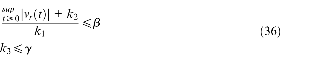
the linear and angular velocity will become
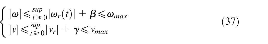
Thus, the linear and angular velocity will never go beyond the limit of the engine.
The stability of the system will be proved as follow.
Proposition 2. If
Proof. Substituting (35) into (31) yields
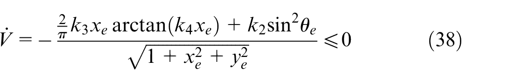
Then, taking the second order derivatives of the Lyapunov function yields
It is already proved that
Substituting the control law of
Since it has been proved that
Block diagram for the control system based on normalisation technique.
Comparison between the proposed control method and model predictive control (MPC)
The method proposed in this paper and the MPC method are both based on the known USV model. However, compared with the MPC method, the proposed controller algorithm has a smaller computational cost and is thus more applicable to a real-time implementation. At each sample time, the MPC method needs to calculate the future states and solve the optimisation problem along the prediction horizon, which requires a powerful and large processor. 32 For the proposed control algorithms, only the current states need to be calculated at each time step, which saves significant computational cost and space.
In addition, conventional MPC requires the existence of a state feedback controller. However, according to Brockett’s condition, a state feedback controller cannot stabilise the underactuated system. 33 Thus, conventional nonlinear model predictive control (NMPC) is not applicable for USVs. To apply NMPC to the control of USVs, many other stringent constraints and condition need to be applied, which adds to the complexity of the control scheme and increases the computation cost.34,35 Besides, some conditions such as forecasting the evolution of the disturbances, etc. are challenging and cannot be achieved in the practical world, which limits the application range of the MPC method. Thus, compared with the MPC method, the proposed controller is more suitable for the real-time trajectory tracking control of USVs.
Simulations
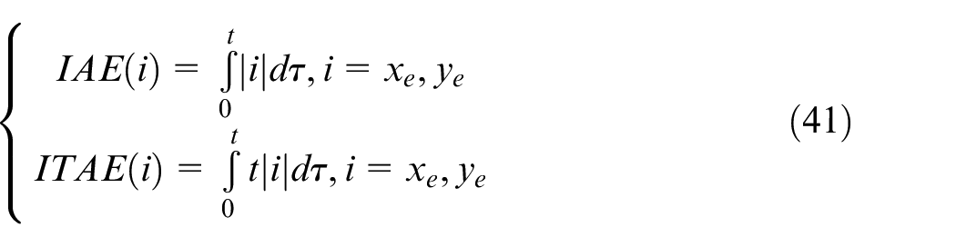
In order to verify the effectiveness of the proposed control schemes for the trajectory tracking control of the USV, simulations are conducted in the MATLAB environment. All simulations were performed on Intel i7 2.60 GHz octa-core CPU with 16 GB RAM. The controllers are tested in four different scenarios: (1) circular trajectory with constant ocean currents, (2) sinusoidal trajectory with constant ocean currents, (3) sinusoidal trajectory with time-varying ocean currents and (4) minimum snap trajectory with time-varying currents. In the fourth scenario, a real case is studied, where the USV is required to pass five stations on the sea to deliver cargos under time-varying ocean currents and berthed at the last stations. The trajectory passing the five stations are generated by the minimum snap method, which produces a smooth and optimal trajectory with a minimum snap under certain dynamic constraints.18,36 Performance comparisons between the two proposed controllers and the PID controllers37,38 are presented in the first scenarios. Then in the rest of the scenarios, only the proposed controllers are tested. Besides, the controller based on the normalisation technique is tested without considering the ocean currents. The result for the controller based on backstepping technology is marked as BS and the controller based on normalisation technique is marked as NL.
The maximum linear velocity and yaw rates are 13 m/s and 0.39 rad/s separately, which are the specifications of a hull craft type ship (shown in Figure 4) in the fleet class.
39
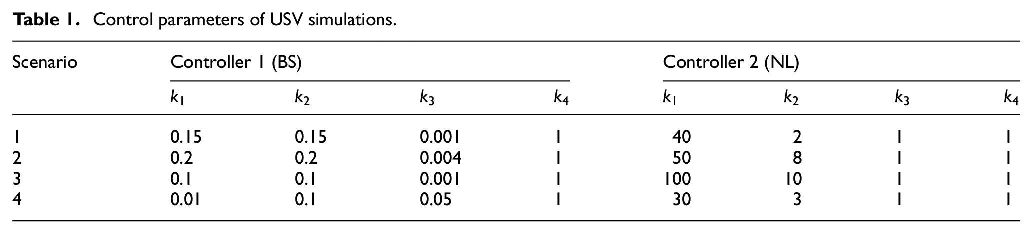
The control parameters of the proposed controllers are listed in Table 1. The simulation time step is set as 0.001 s. The initial condition for the actual USV is set as
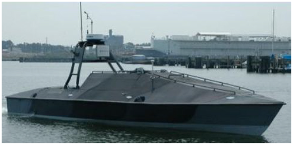
A hull craft type ship in the fleet class. 40
Control parameters of USV simulations.
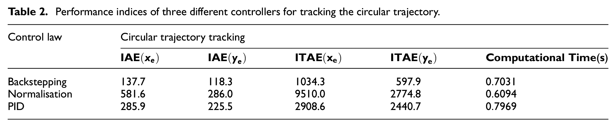
Performance indices of three different controllers for tracking the circular trajectory.
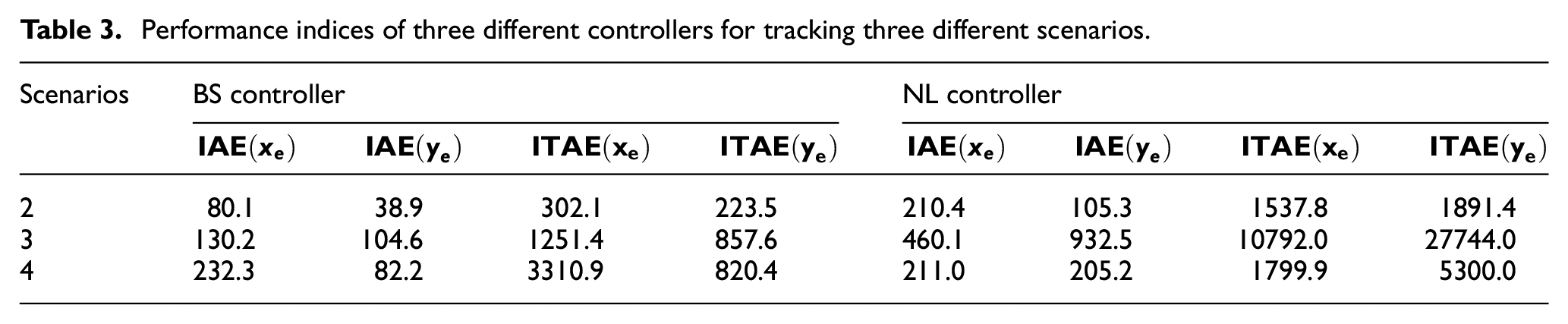
Performance indices of three different controllers for tracking three different scenarios.
Circular trajectory with constant ocean currents tracking simulation
The desired trajectory for circular trajectory tracking simulation is given as
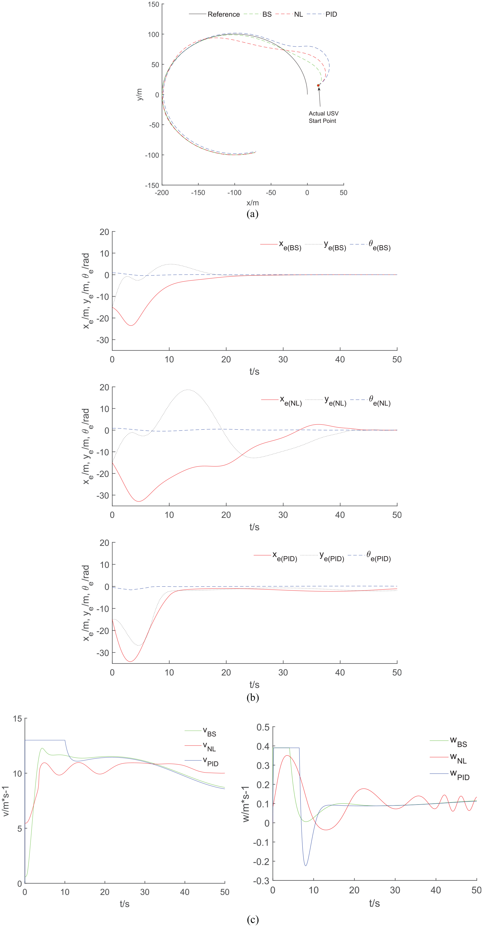
Result for the circular trajectory: (a) circular trajectory tracking, (b) tracking errors for the circular trajectory and (c) linear and angular velocity for the circular trajectory.
The detailed distinction of the steady-state and transient performance is more clearly shown in Figure 5(b) and Table 2. As it is shown in Figure 5(b), the PID controller cannot eliminate the steady-state error, which leads to poor trajectory tracking precision. In contrast, there is no steady-state error for the proposed controller. Moreover, compared with the PID controller, the BS control systems have smaller transient tracking errors, settling time, IAE and ITAE. Therefore, BS control drives the USV to track the circular trajectory more quickly and precisely and has a superior steady state and transient performance. It is also demonstrated that the BS controller can handle the ocean currents, while the PID controller fails to tackle it. Figure 5(c) shows that the input of all the controllers is within the saturation limit. The two proposed controllers produce smoother and smaller inputs than the PID controller. With respect to the computational cost, although the PID controller requires a shorter running time than the proposed controller, the time difference between them is not obvious. Furthermore, between the two proposed controllers, the BS controller is more aggressive than the NL controller, resulting in sharper changes, especially when the tracking error is large. BS has better transient and steady state performance with less smooth inputs than the NL controller.
To sum up, compared with the PID controller, the proposed controllers have higher trajectory accuracy, better transient and steady state performance, less power consumption and close computational cost. For the proposed BS and NL controllers, the computation time for each time step (0.001 s) are only
Sinusoidal trajectory tracking with constant ocean currents simulation
A reference trajectory with varying linear and angular velocity are tracked in this simulation. The desired trajectory for the sinusoidal trajectory tracking is given as
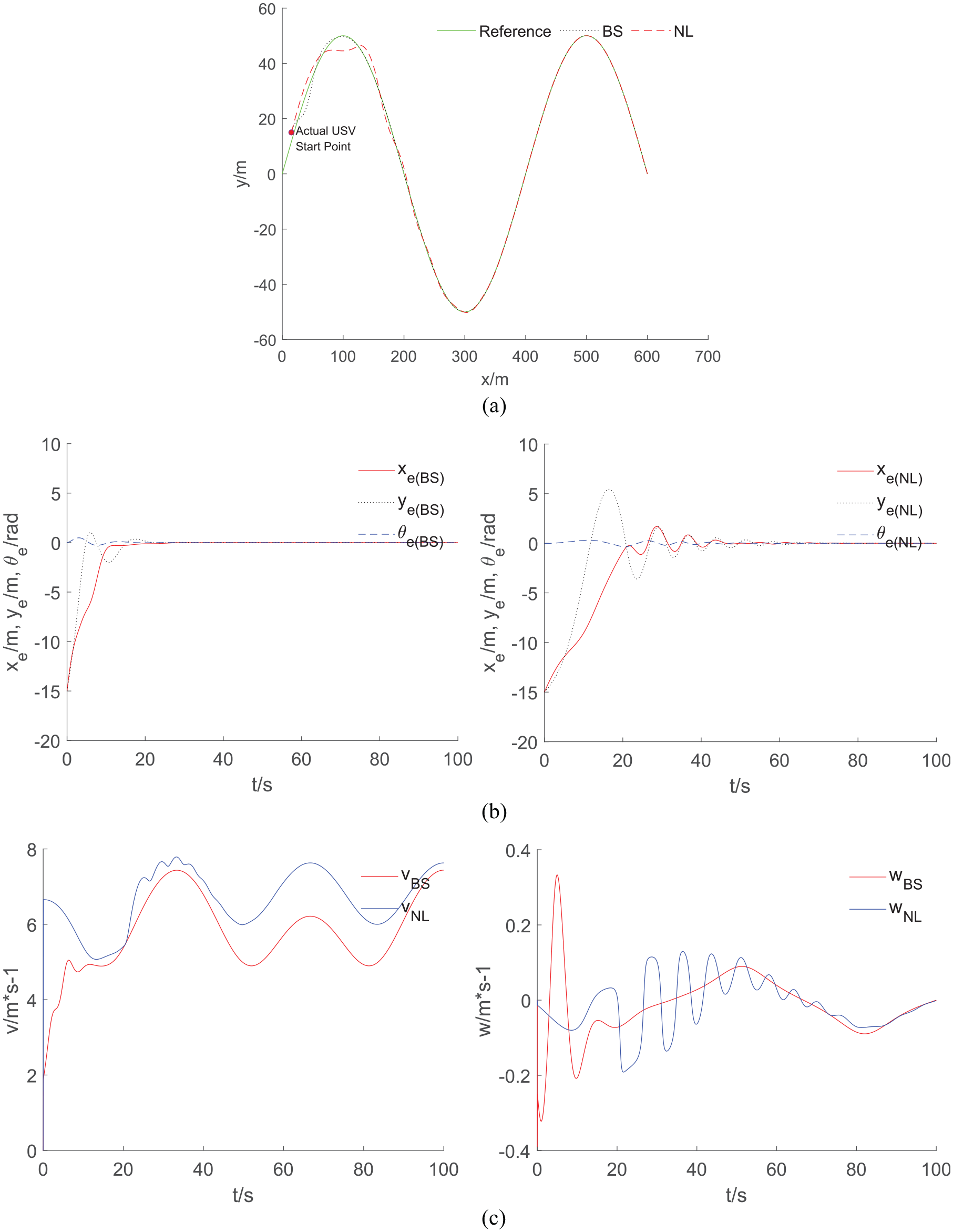
Simulation results for the sinusoidal trajectory: (a) sinusoidal trajectory tracking, (b) tracking errors for the sinusoidal trajectory and (c) linear and angular velocity for the sinusoidal trajectory.
Sinusoidal trajectory tracking with time-varying ocean currents simulation
In this scenario, a more complicated sinusoidal trajectory with sharper change and time-varying ocean currents are tested. The reference trajectory is given as
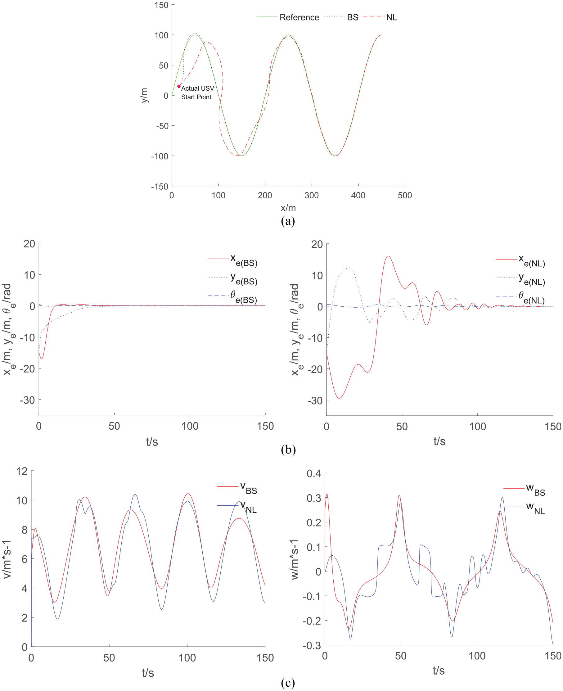
Sinusoidal trajectory with time-varying ocean currents: (a) sinusoidal trajectory with the time-varying ocean current, (b) tracking errors for sinusoidal trajectory with time-varying ocean currents and (c) linear and angular velocity for sinusoidal trajectory with time-varying ocean currents.
Minimum snap trajectory with time-varying ocean currents simulation
Here, a complex minimum-snap trajectory requiring the USV to smoothly pass through four stations and stop at a final station is presented. The position of the starting point and the five stations are set randomly as
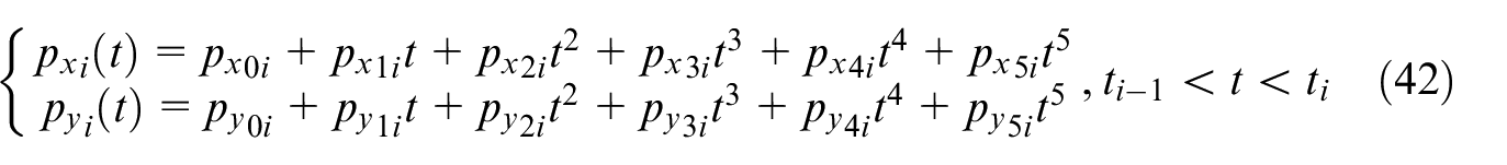
where
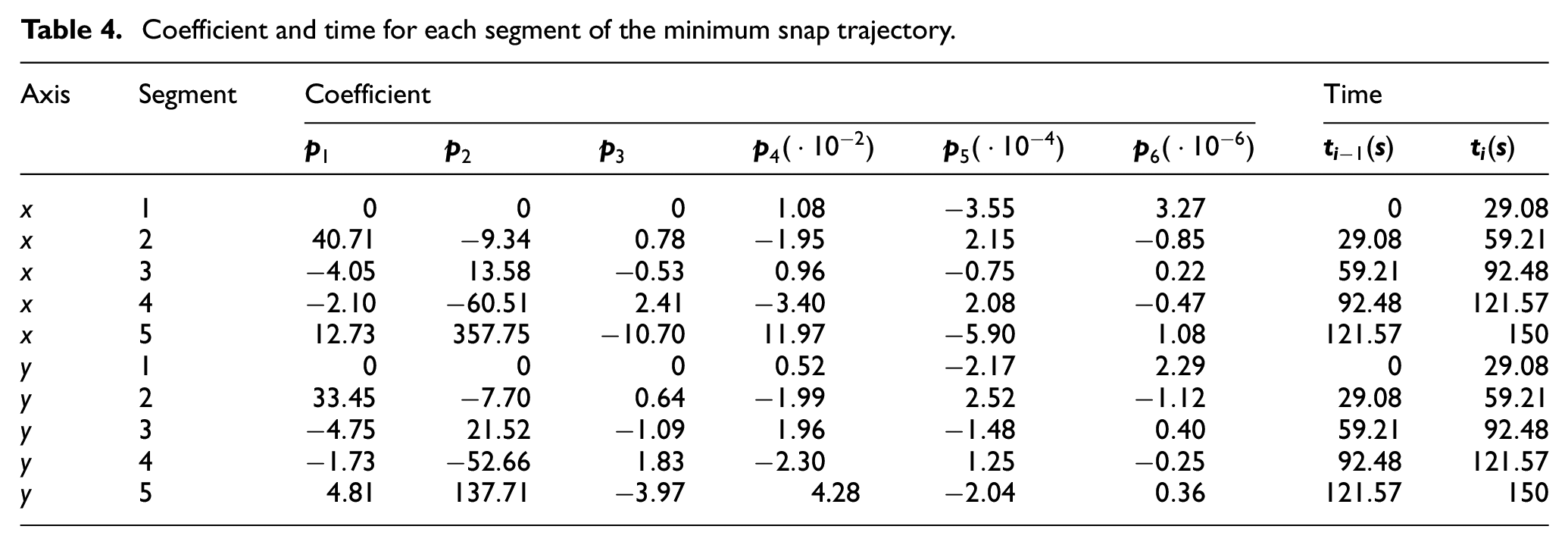
The corresponding coefficient and time for each segment are shown in Table 4. The results from the test are shown in Figure 8 and Table 3. These figures show that convergence of the tracking errors can be guaranteed for the complicated minimum snap trajectory by both two controllers. However, the USV controlled by the NL controller missed the first station, thus failing to meet all the target. The BS controllers converge more quickly and can tackle the ocean currents, while the NL controller produces smoother inputs. Both controller algorithms are efficient in a realistic and challenging case study.
Coefficient and time for each segment of the minimum snap trajectory.
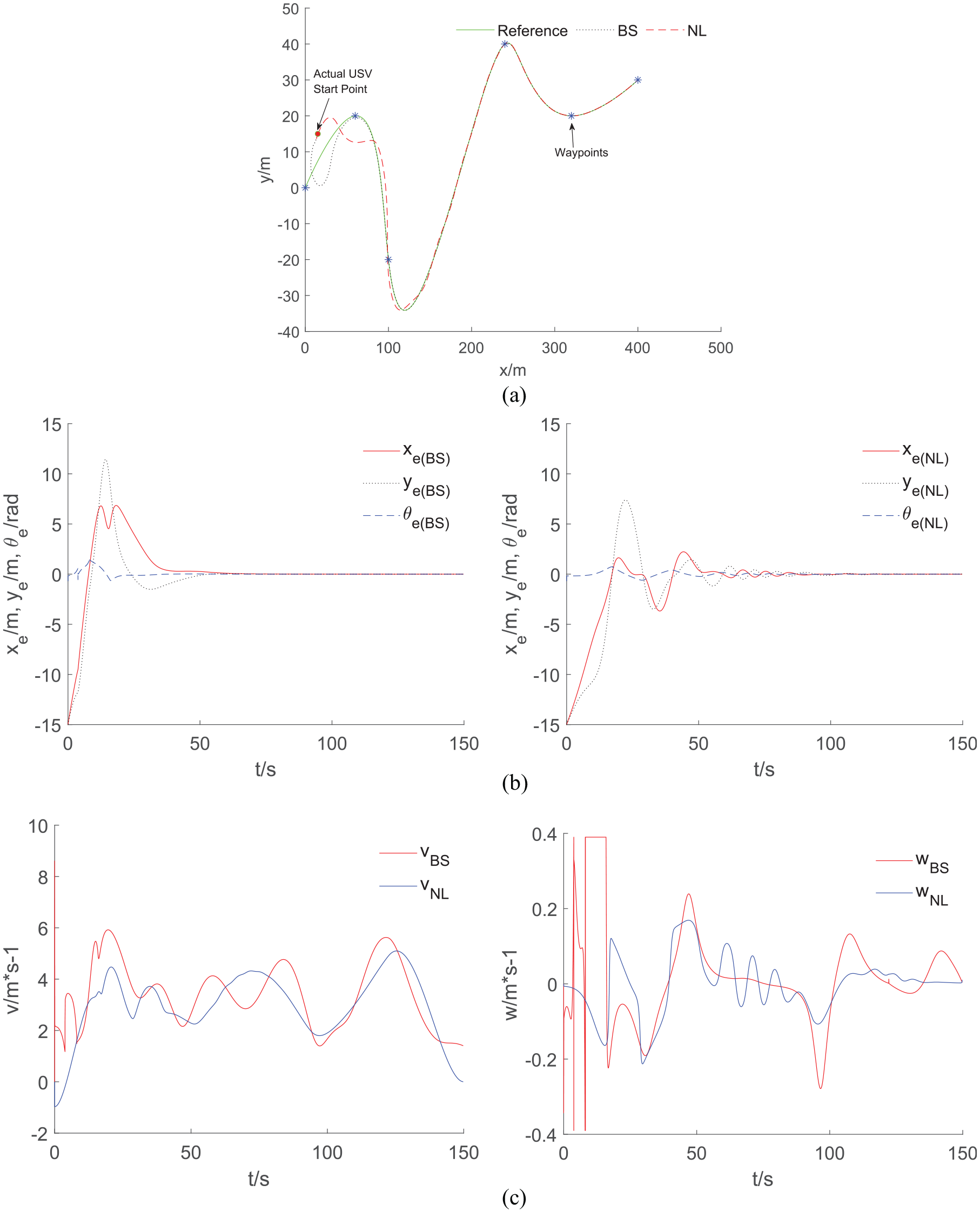
Minimum snap trajectory with time-varying ocean currents: (a) minimum snap trajectory with the time-varying ocean current, (b) tracking errors for sinusoidal trajectory with time-varying ocean currents and (c) linear and angular velocity for sinusoidal trajectory with time-varying ocean currents.
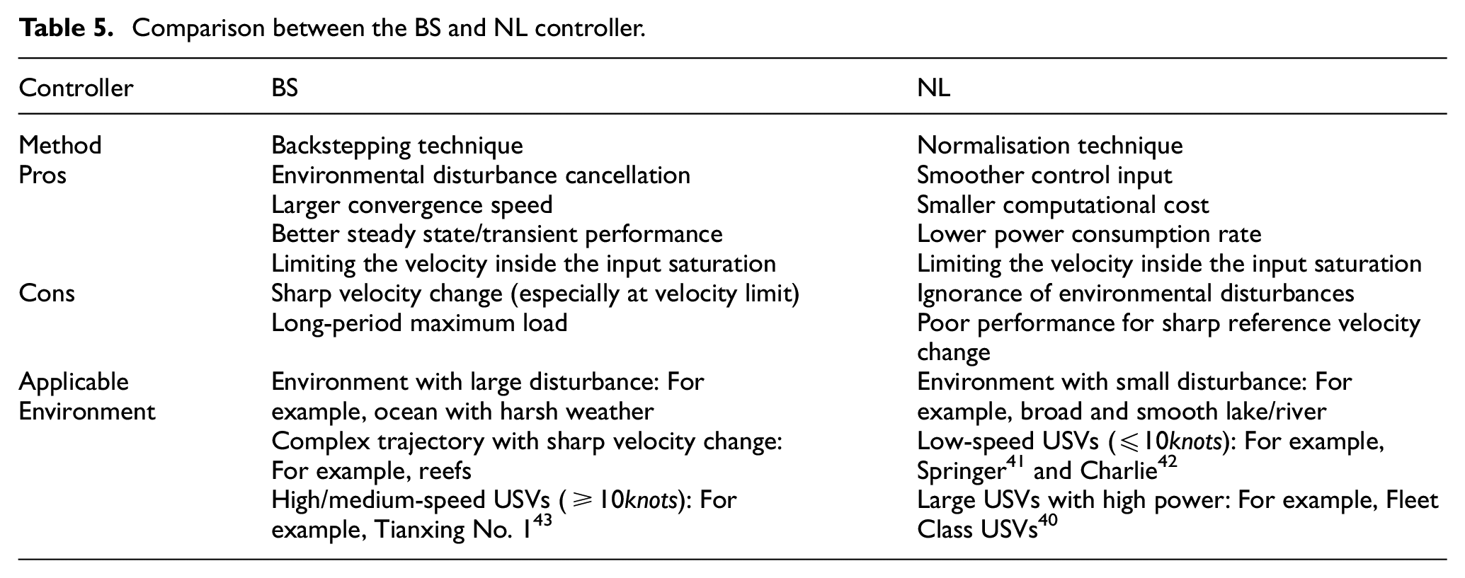
In conclusion, both two proposed controllers can converge the USV to the desired reference trajectory with the velocity limited inside the input saturation. The BS controller has superiority in convergence speed, steady-state performance and transient performance. Moreover, it can cancel the time-varying environmental disturbances. The NL controller produces smoother input, requires smaller computational cost but is incapable of handling the environmental disturbances. The detailed comparison between the two controllers is listed in Table 5.
Comparison between the BS and NL controller.
Conclusion and future works
This study investigates the control methods for trajectory tracking control with motion constraints and environmental disturbances. For handling the disturbance, a virtual system is proposed to simplify the USV model and compensate for the environmental disturbance. Then, based on the virtual system, the backstepping technique and Lyapunov direct method are used to calculate the control law and the motion constraints is handled by an auxiliary system. The proposed controller has a limited ability to handle input saturation. Thus, a new controller based on normalisation is designed. The tracking error is normalised in this controller and the velocity will be related to the reference and design parameters only, so that the controller can produce smoother velocity inside the motion constraints. Both controllers are able to force the USV to track the desired trajectory and handle the input saturation. Additionally, it is proved that through the use of a virtual system, even under harsh environmental disturbances like time-varying ocean currents, the system is still able to track a complicated trajectory. Moreover, the proposed controller performs better than the common adaptive controller when the ocean currents are measurable. The two proposed methods can guarantee the unformal stability of the closed-loop system. Simulation results verify the effectiveness of the two controllers in commanding a USV for a range of trajectories and ocean current conditions. Therefore, the introduced solutions enable USVs to follow complex trajectories in a harsh marine environment.
Future work will include incorporating the dynamic model in the design of the controller, with the dynamic uncertainties taken into consideration, as well as increasing the speed of the stabilisation action and smoothness of the inputs of the controllers. Experiments of the USV controlled by the proposed control scheme in a complex environment will also be conducted to validate the effectiveness of the algorithms and study the real-time performance. Besides, the state constraints may also be taken into consideration and solved potentially by the Barrier Lyapunov function (BLF).
Another important research direction is to investigate the control of USVs complaint with COLREGs, which is an international traffic regulation for preventing collisions at sea. A plausible strategy to achieve this is to integrate sensing and planning modules with the controllers. For example, an appropriate moving obstacle detection system (based upon radar, AIS or visual systems) should be first investigated to capture the navigational information of moving ships in real-time. Then, the collision risks should be properly assessed by using DCPA/TCPA 44 or ship domains, 45 which will facilitate path planning algorithms to generate COLREGs compliant collision free trajectories and enable path following controllers to track.
It also should be noted that before real implementation, the proposed trajectory tracking control solution will need to be complemented with collision avoidance approaches. In particular, the extension to multi-agent systems will require the consideration of both internal and external obstacles, with many alternative methods being applicable for formation control and cooperative motion planning. Specific strategy could be that the artificial potential field method 46 can be first implemented to model and evaluate the collision risks imposed by obstacles. Path planning algorithms such as the constrained A* algorithm 47 will then be employed to generate collision free trajectories, which will finally robustly be tracked using the controller developed in this paper.
Footnotes
Declaration of conflicting interests
The author(s) declared no potential conflicts of interest with respect to the research, authorship, and/or publication of this article.
Funding
The author(s) disclosed receipt of the following financial support for the research, authorship, and/or publication of this article: This work is partially supported by Royal Society (Grant no. IEC\NSFC\191633).