
Abstract
Current practices of condition assessment in large marine engines are largely based on the measurement of cylinder pressure using external kits, which poses challenges due to sensors synchronisation and durability issues, as well as the inability to perform continuous monitoring. For addressing these challenges, this study aims at developing a novel method to solve the inverse problem of predicting the pressure variations in all engine cylinders, by using the Instantaneous Crankshaft Torque (ICT) measurement for large internal combustion engines. This method is developed by considering the Initial Value Problem (IVP) technique along with the integration of a direct crankshaft dynamics model incorporating the sensitivity parameters and stability criteria calculation based on the Lyapunov Exponent (LE) as well as a state-of-the-art Nonmonotone Self-Adaptive Levenberg-Marquardt (NSALMN) optimisation algorithm. The method is tested for a number of case studies using different combustion models based on the Weibe and sigmoid functions, as well as for healthy, degraded and faulty engine conditions. The derived results demonstrate adequate accuracy exhibiting a maximum error of 0.3% in the prediction of the mean peak in-cylinder pressure. The analysis of the calculated sensitivity parameters resulted in the identification of the parameters that significantly impact the solution, thus providing improved insights for selecting the developed method settings. The developed method renders the continuous and non-intrusive in-cylinder pressures monitoring feasible, by using a permanently installed shaft power metre sensor with higher sample rates.
Keywords
Introduction
Large two-stroke diesel engines are by design the most efficient internal combustion engine type, 1 and as a result they are employed in a variety of ship propulsion and power generation applications.2,3 However, under actual operating conditions, degradation effects and various faults significantly reduce the engine efficiency and availability, whilst leading to increased emissions and operational costs.4–6 With the advent of digitalisation, monitoring and analysing various engine parameters, such as engine power, fuel consumption, working medium temperatures, scavenge air pressure and in-cylinder pressures, have become widespread among engine operators.7,8 In this way, better insights for the engine’s condition can be obtained, which prompts maintenance and repair actions in order to attain the engine optimal efficiency and reliability as well as to reduce the associated operating cost and gaseous emissions, with tangible benefits on the ship operations sustainability. 9
Amongst the most prominent indicators for the engine condition is the measurement of the in-cylinder pressure, 10 as it provides information to analyse the combustion process quality,11,12 blowby, 13 cylinder misfire and knock,14,15 cylinder compression ratio and injection timing, 16 as well as injector degradation and failures. 17 However, the methods currently employed in determining all of the above, rely on direct measurements of the in-cylinder pressure by deploying pressure sensors to either one or multiple cylinders, which can be expensive, suffer from poor durability,18–20 exhibit synchronisation issues 21 and most often do not allow for continuous monitoring. Nonetheless, recent technological improvements have led to the development of continuous pressure monitoring systems which are primarily utilised in high-value power plants, such as those with dual-fuel engines. 22 However, for the majority of typical large internal combustion engines such as those employed in the 62,100 ocean-going vessels world wide, 23 the costs involved with such monitoring systems remain outside the reach of most shipowners and operators. 24 Moreover, having measured the in-cylinder pressure, the non-trivial task of signal correction is required, in order to remove the noise and perform averaging over several cycles, and most importantly to remove offsets by calibrating the acquired signal with respect to the engine crank angle 25 and the cylinder pressure. 26
As a result, methodologies have been developed utilising alternative engine measurements to predict important features that belong to, or can be directly derived from the in-cylinder pressure diagrams in a reliable and low-cost manner. In specific, for automotive industry applications, the peak pressure position has been predicted using accelerometers mounted on every cylinder,27,28 as well as an ICT sensor. 18 Furthermore, properties such as the burned mass fraction and combustion phasing were estimated by utilising measurements from an ICT sensor 29 and an Instantaneous Crankshaft Speed (ICS) sensor. 30 Regarding large diesel engines, limited applications of such methodologies can be found in the pertinent literature. In particular, for a slow speed two-stroke diesel engine, the indicated power in each cylinder was estimated by employing ICT sensor measurements with a black-box ANN model. 31 For high and medium speed four-stroke diesel engines, ICS sensor measurements were used to detect individual cylinders misfiring, 32 and diagnose fuel pump faults through in-cylinder pressure differences, respectively. 33
In addition, further advances have been made by developing methodologies, which attempt to reconstruct the entire in-cylinder pressure diagram. Regarding automotive applications, engine block vibration signals were utilised,34–36 however the signal quality is very sensitive to the sensors’ placement, which is often decided arbitrarily. 37 Inverse physical modelling has also been utilised along with an ICS sensor,19,20 however the inversion of a purely physical (white-box) crankshaft dynamics model presented challenges due to singularities occurring at the piston Top Dead Centre (TDC). To resolve such inversion problems, a grey-box model was developed utilising the ICS along with the measured in-cylinder pressure in one of the engine cylinders, in order to estimate the in-cylinder pressure in the remaining engine cylinders. 38 Regarding larger diesel engines, only one application has been identified in the literature, which attempts to reconstruct the in-cylinder pressure diagrams of all cylinders of a large two-stroke diesel engine. 39 For this case, the in-cylinder pressure function was parametrised by using two parameters; the polytropic expansion coefficient and a pressure amplitude factor. Hence, it remains uncertain whether by this method, the in-cylinder pressure can be predicted accurately in case of existing engine faults or degradation. Subsequently, the parametrised in-cylinder pressure was used along with the ICT sensor measurements as part of a grey-box model, that resulted in a maximum error of 12% for the in-cylinder pressure prediction. However, a change of 5% in peak in-cylinder pressure is sufficient to cause a substantial impact in engine performance, 40 hence a method with smaller error tolerances is required.
It is deduced from the preceding discussion that three peripheral measurements (the engine block vibrations, ICS and ICT) have been used to establish a robust relationship with the in-cylinder pressure. In specific, the engine block vibration signals carry substantial non-pressure related information, which significantly complicates the analysis. 41 On the other hand, the ICS measurement (raw signal from the angle encoder) requires post processing, a comparatively higher sampling rate compared with the ICT measurements to capture the instantaneous shaft rotational speed with adequate accuracy, and exhibits a low signal to noise ratio. 31 Hence, the ICT forms a better choice compared to the engine block vibration and ICS measurements, due to its higher signal to noise ratio as well as its linear response with engine load for the case of large two-stroke engines. 42
Therefore, from the preceding literature review, the following gap has been identified: there exists no methodology for large two-stroke diesel engines, which can predict the in-cylinder pressure using peripheral measurements, firstly for the cases of degraded or faulty engine operation, and secondly with adequate accuracy for the case of healthy engine conditions. In this respect, the aim of this study is to develop a method that utilises the ICT measurement from a single torque sensor, to predict the in-cylinder pressures pressure variations for every engine condition including healthy, and various faulty or degraded conditions, thus potentially offering a reliable and low cost solution for a continuous pressure monitoring system. To accomplish this aim, this study employs the extension of a direct crankshaft dynamics model, the parametrisation of the in-cylinder pressure function, the development of an appropriate inverse problem method and its implementation to predict the in-cylinder pressure for a number of realistic engine operating conditions.
Methodology
The methodological steps followed in this study are listed below:
Description of the reference system and the direct crankshaft dynamics model. This model is employed in step 3 as part of the inverse problem method, and in step 6 to simulate the engine ICT for healthy, faulty and degraded conditions.
Determination of the parametrised in-cylinder pressure functions, and selection of parameters to be estimated by the inverse problem method.
Derivation of sensitivity equations, to be utilised for the development of the inverse problem method in step 5.
Development of the inverse problem method, which estimates the in-cylinder pressure parameters by utilising ICT measurements.
Implementation of the inverse problem method for a number of case studies for validation and testing under various engine operating conditions. This is performed by using the direct crankshaft dynamics model for the reference system, to simulate the ICT measurements for healthy, faulty and degraded engine conditions.
Discussion and analysis of results.
Reference system and direct crankshaft dynamics model
The reference system used in this study is a large two-stroke diesel engine driving a generator, which operates at a nominal speed of 124 r/min. The engine has 10 cylinders with an inline configuration, and a Maximum Continuous Rating (MCR) of 15.5 MW. For developing the crankshaft dynamics model of this system, 16 degrees of freedom are considered, which represent the 3 masses within the engine torsional damper, the 10 engine cylinders, the engine camshaft drive, the engine flywheel and the electric generator rotor, as shown in Figure 1.
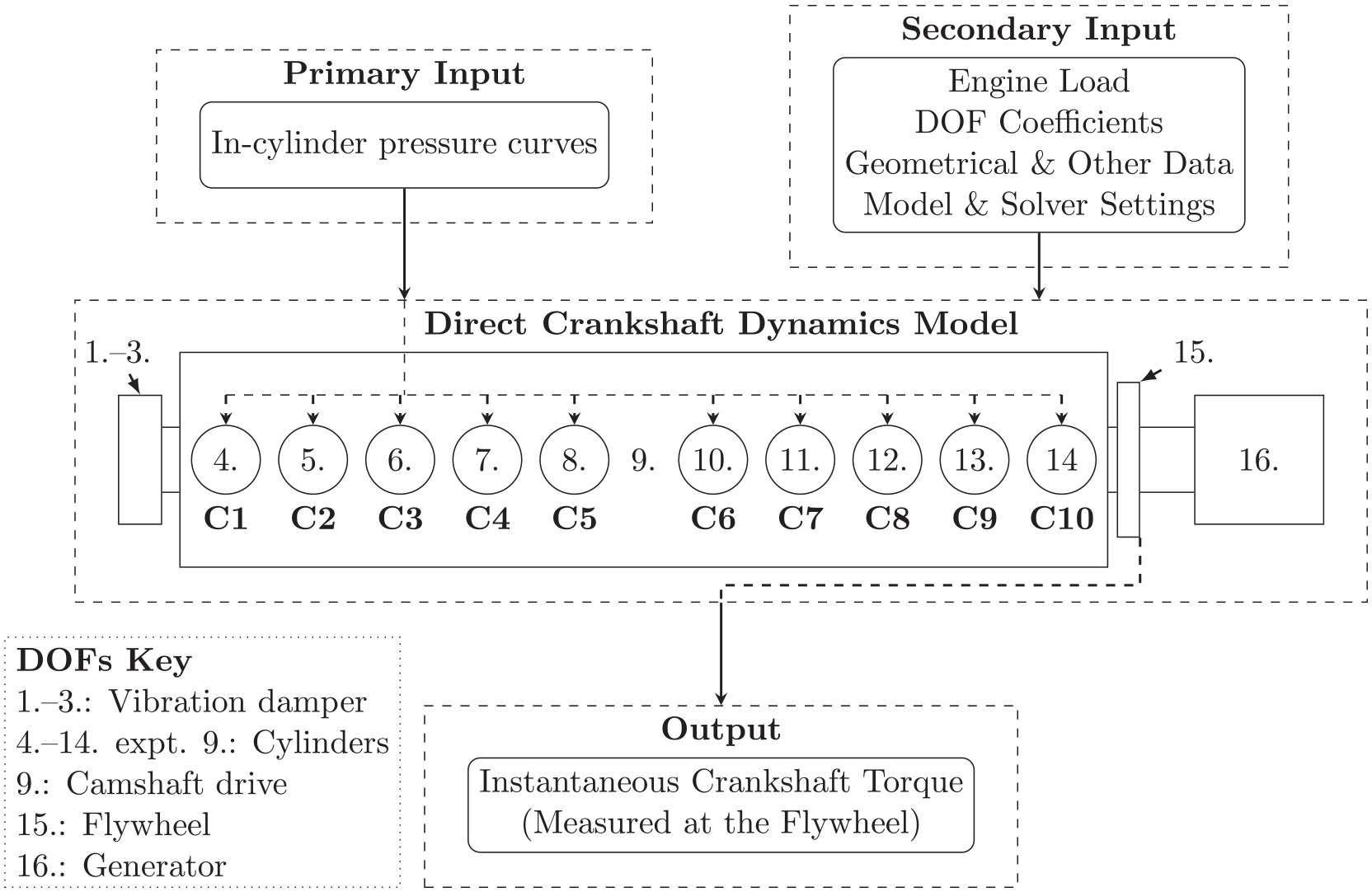
Schematic of the direct crankshaft dynamics model.
A direct crankshaft dynamics model is utilised in this study. This model has been developed, validated and employed to investigate the reference system response considering various friction submodels and solver settings in a previous authors’ study. 43 In this study, this model is employed to firstly develop the inverse problem method in Section Inverse problem method development, and secondly to provide the required input of ICT at the flywheel for the case studies presented in Section Case studies design. The direct model is of the lumped parameter type consisting of 16 Degrees of Freedom (DOFs), and uses as primary input the in-cylinder pressure diagrams for each cylinder, and as secondary input the engine load, the DOFs inertia, damping and stiffness coefficients (obtained from the engine torsional vibration analysis), the geometrical and other data obtained from the manufacturer documentation, as well as the settings (solver and submodels) defined by the user, as shown in Figure 1. Furthermore, the direct model is based on a system of 16 non-linear second order differential equations, the solution of which is used to calculate the ICT at the engine flywheel according to equations (1) and (2), respectively. These equations will also be employed for the development of the inverse problem method.
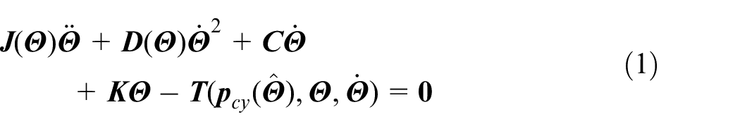

In equation (1),
In-cylinder pressure parametrisation
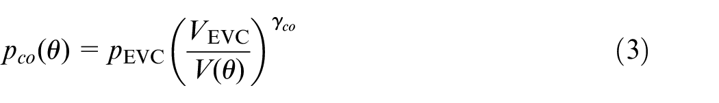
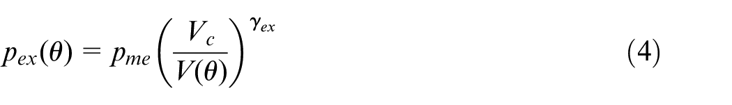
The parametrisation of the in-cylinder pressure curve for the closed part of the diesel cycle is a critical task. Therefore, the cylinder pressure curve should be adequately parametrised, such that faults or degradation is captured by changing the employed parameters. Moreover, the parametrised in-cylinder pressure function should employ as few parameters as possible, in order to reduce the mathematical and computational complexity. The engine in-cylinder pressure curve can be parametrised by using semi-empirical equations, which have demonstrated high accuracy and low computational complexity.44–46 In specific, this is accomplished by using different equations to represent the three main in-cylinder processes (compression, combustion and expansion). The compression and expansion processes are modelled using polytropic relationships according to equations (3) and (4), whilst the combustion process is modelled by using a function that interpolates between the other two processes.18,46 Hence, by considering the interpolating function, the analytic in-cylinder pressure function for the closed cycle is represented by equation (5).

The parameter
For a diesel engine, there are two types of interpolating functions which can be used in equation (5). The most simplistic one is the sigmoid function, 48 since it depends on two parameters according to equation (6). The second one is the single Weibe function, which is extensively used in combustion modelling applications,46,47,49 and is represented by equation (7).

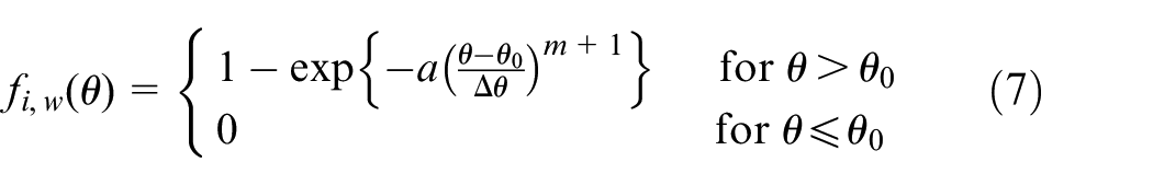
For the sigmoid function,
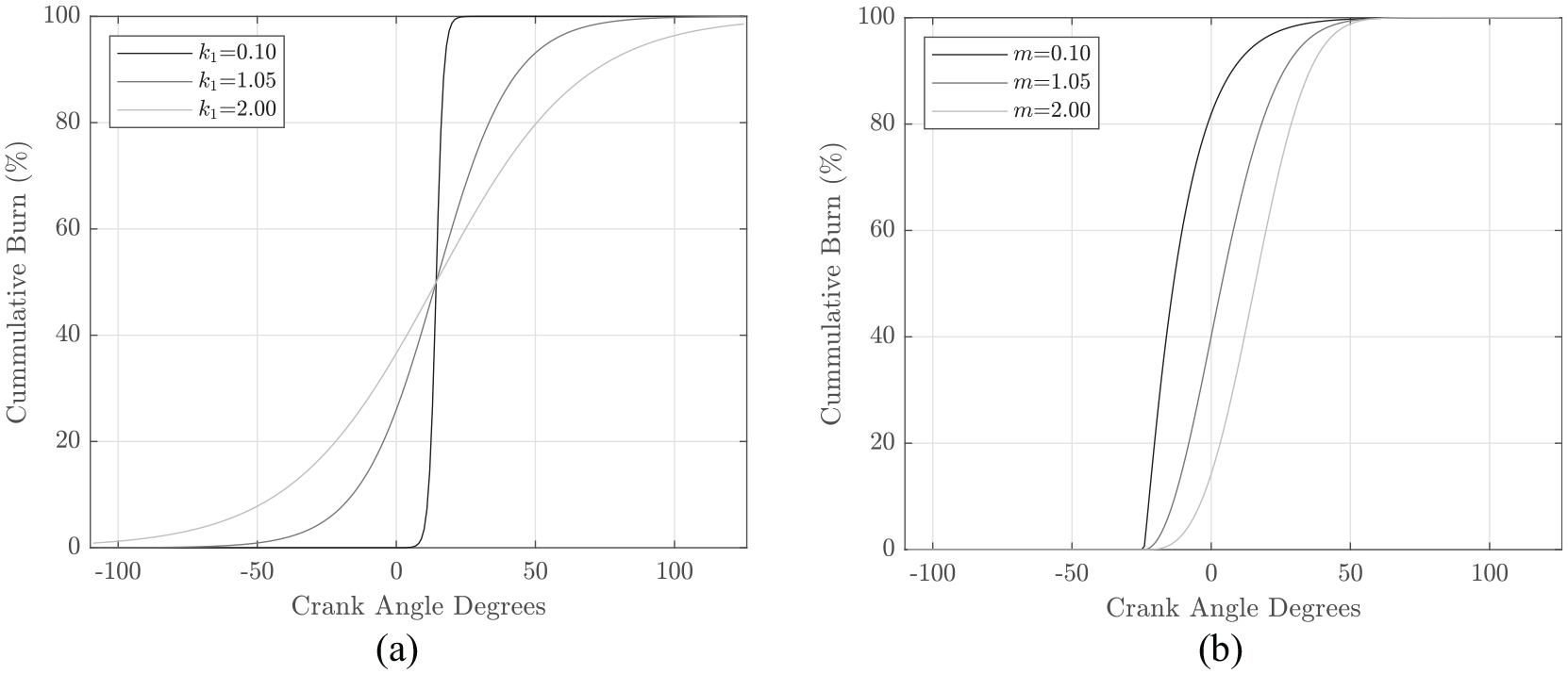
(a) Sigmoid functions with different
The performance of the inverse problem method is evaluated for both interpolating functions as described in Section Case studies design.
Having obtained the equations (3)–(7), each of their included variables can be classified as known or unknown parameters, as summarised in Table 1. This information will be employed in Sections Sensitivity and stability analysis and Inverse problem method development, so that the sensitivity equations and subsequently the inverse problem method can be formulated accordingly, in order to estimate the values of the unknown parameters. The parameters classified as known are the ones, which are either known a priori, can be obtained from basic manufacturer documentation, or can be easily measured on site using existing permanently installed sensors. In specific, these parameters belong to equations (3) and (4) and include the in-cylinder pressure at the exhaust valve close position (
Pressure function parameters classification.
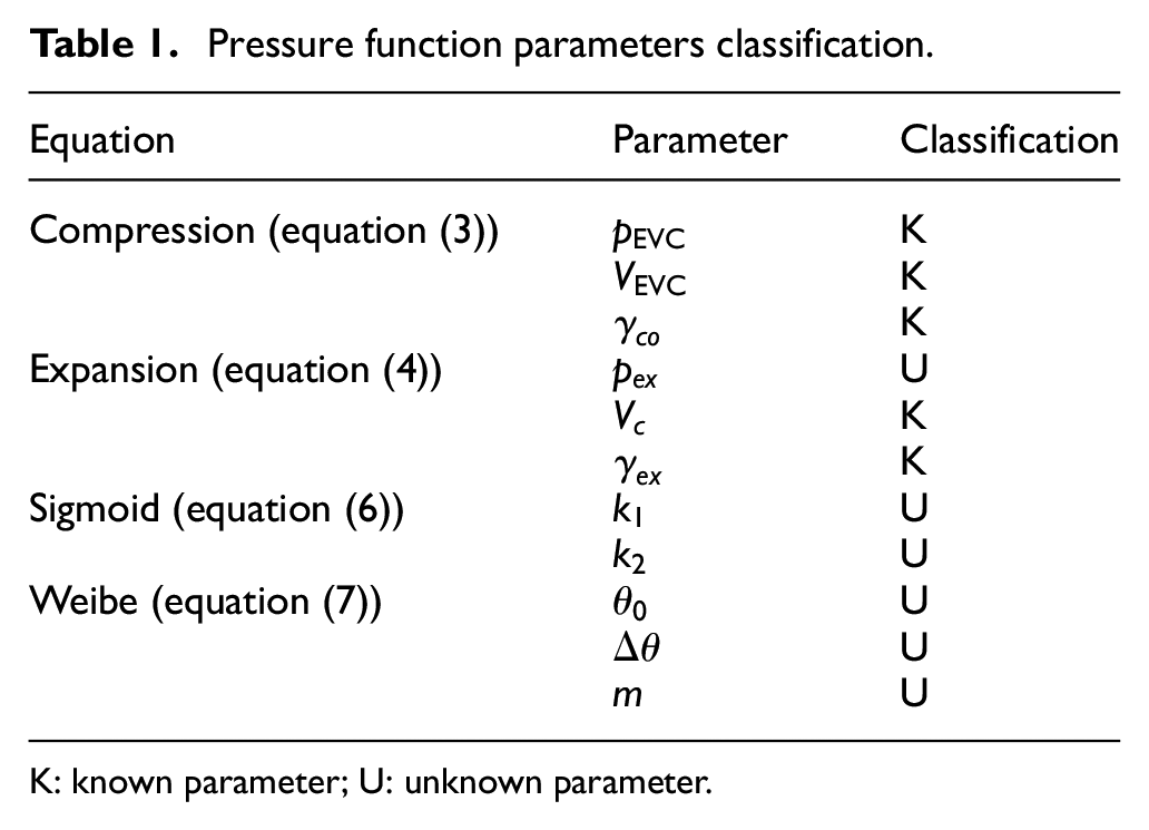
K: known parameter; U: unknown parameter.
The parameters classified as unknown are the ones that their values will be estimated in this study, by using the ICT measurement. These parameters greatly effect the shape of the in-cylinder pressure diagram and can only be estimated using the in-cylinder pressure measurements, which are associated with inherit drawbacks, as explained in Section Introduction. In specific, the unknown parameters are, the maximum expansion pressure (
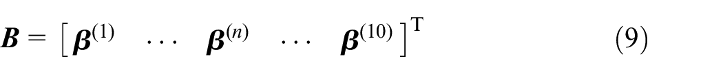
The parametrised in-cylinder pressure function (equation (5)) can be incorporated to the direct model governing equations (equation (1)). This is firstly performed by grouping the unknown parameters for the n th cylinder into a parameter vector
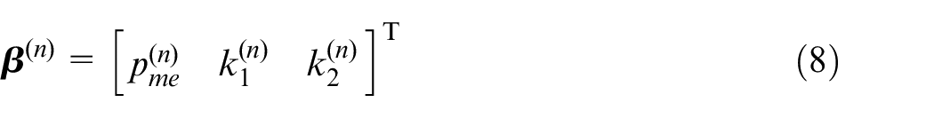
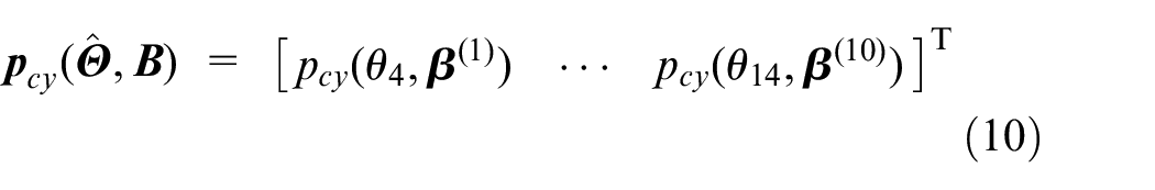
Subsequently, the direct model governing equations have become functions of the unknown parameters vector
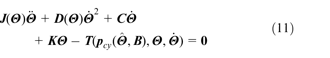

It should be noted that the angular displacement, velocity and acceleration vectors are functions of time and
Sensitivity and stability analysis
The sensitivity equations are employed in order to determine the rate of change of a differential equation’s solution, with respect to specific parameters of that differential equation. 53 In specific, the sensitivity equations are useful when, as it is often the case, a closed-form expression of the differential equation response is not available, hence symbolic differentiation cannot be directly performed. In this study, the sensitivity equations are used in order to calculate the objective function gradient, and to perform the stability analysis, which warns the user of possible chaotic behaviour when implemented within the inverse problem method, as described in Section Inverse problem method development .
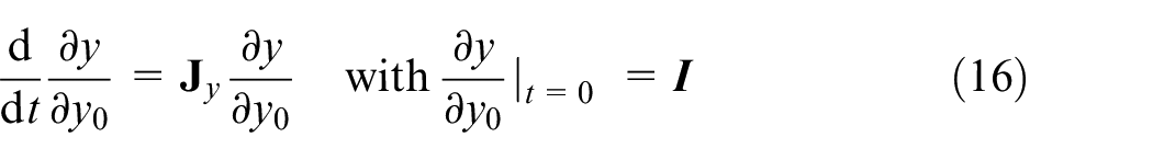
Thus, in order to aid the derivation of the aforementioned sensitivities, the generic form of the sensitivity equations should be obtained first given an arbitrary differential equation, in accordance to equations (13)–(15): 53

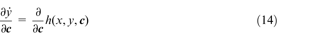
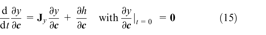
Equation (15) is a first order linear differential equation with variable coefficients, which is solved for the dependent variable
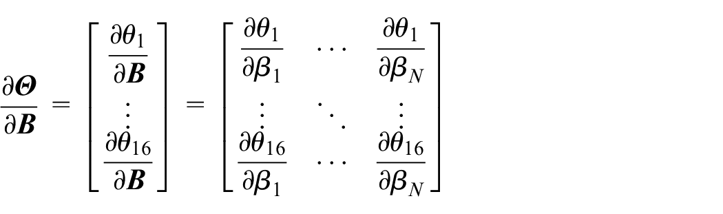
Following the above, the sensitivity equations for this study will be firstly derived with respect to the unknown parameters vector
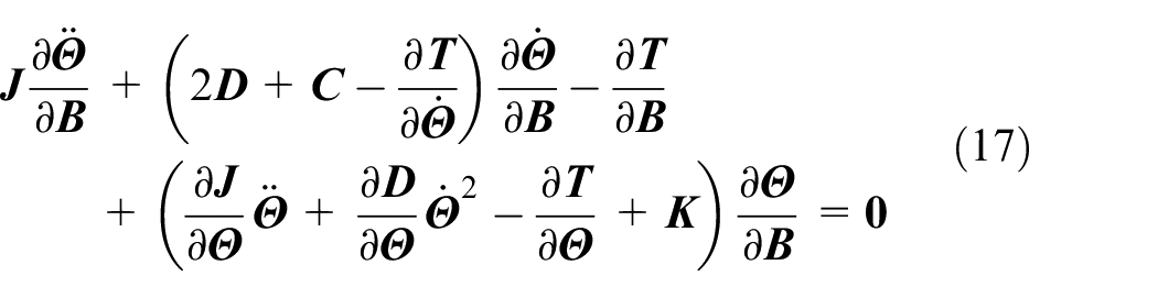
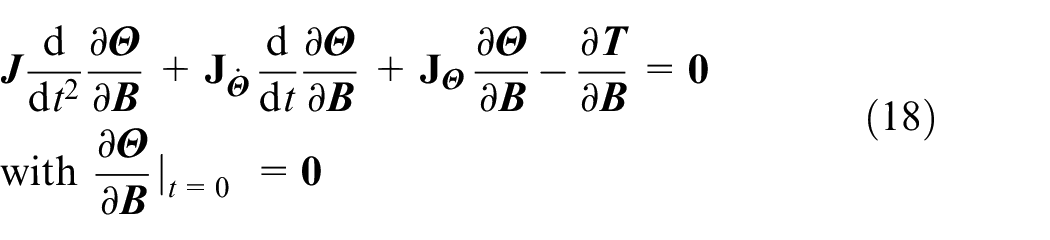
Equation (18) is a linear second order differential equation with variable coefficients, where
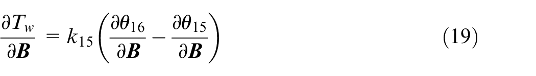
As a result, the sensitivity of the flywheel torque
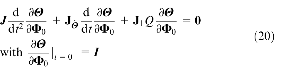
To analyse the stability of the solution from equation (11), the local sensitivity with respect to the direct model initial conditions
By utilising the solution of equation (20), the stability of the system of equations can be quantified by using the Lyapunov Exponents (LE). 54 In specific, the LE is provided in accordance to equation (21), and it quantifies the average exponential rate of divergence of nearby solutions from a given current solution, which is obtained provided a set of initial conditions.
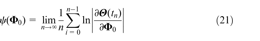
Therefore, the case where the LE exists and is positive implies that nearby solutions will diverge from the current solution if a small change in the initial conditions is introduced. Consequently, there exists a very sensitive dependence of the differential equations solution with respect to the initial conditions. In contrast, negative values of the LE imply that changes in initial conditions will eventually converge to the current solution given a sufficiently large length of time. Hence, the solution is deemed insensitive to changes in the initial conditions. In this case, a smaller value of the LE denotes a faster convergence to the current solution.
Extended direct crankshaft dynamics model
Having derived the sensitivity equations in the previous section, it is observed that the values for their variable coefficients depend on the solution of the direct model governing equations. Therefore, it is common practice when employing the sensitivity equations to solve them simultaneously with the original model equations, in order to enhance the computational efficiency of the solution procedure. 55 As a result, the governing and the sensitivity equations can be simultaneously solved as part of an extended version of the direct crankshaft dynamics model, hereinafter referred to as the extended model.
In particular, the direct model shown in Figure 1 is extended such that it can provide as output the following two sensitivities: the flywheel torque with respect to the unknown parameter vector (equation (19)), and the solution of equation (11) with respect to the initial conditions (equation (20)). The former sensitivity is used for the objective function gradient calculation as described in Section Inverse problem method development, whereas the latter is used to perform the stability analysis as described in Section Sensitivity stability analysis. The extended model is therefore configured to calculate both sensitivities as shown in Table 2, so either one or both can be derived as output by the user as required. Moreover, it should be noted that the model input remains the same for the extended model as it was for the direct model.
Direct and extended model output; extended model input remains the same as the direct model.
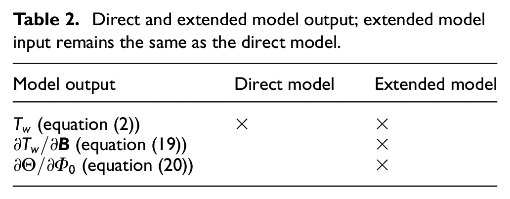
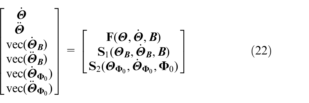
The extension of the direct model is accomplished by firstly transforming the governing equations and the two sets of sensitivity equations into a pseudo-explicit form. This implies that the aforementioned equations are transformed, such that their left hand side is a vector that consists of the first and second dependent variables’ time derivatives. For this, the vectorisation operator
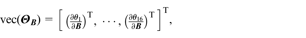
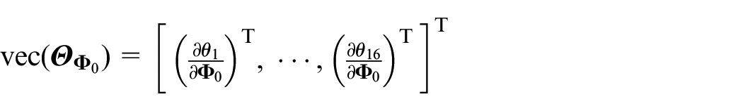
Since the time derivative is a linear operator where
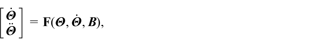
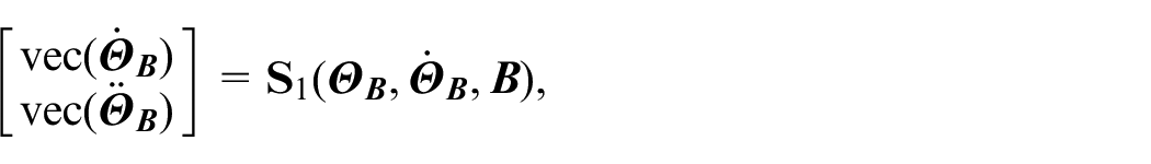
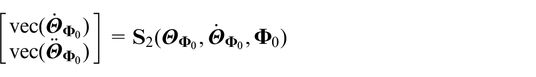
where system of equations
Inverse problem method development
Optimisation algorithm selection
The inverse problem method is the means of accomplishing the aim of this study, that is predicting the in-cylinder pressures based on the ICT measurement. The development of this method is based on the selection of an optimisation algorithm, and subsequently, it is implemented by combining this algorithm with the extended crankshaft dynamics model, as described further below in this Section. In specific, as explained in Section Reference system the direct model, the in-cylinder pressure is used as the primary input to the direct crankshaft dynamics model to predict the engine ICT. In the inverse problem method, the measured ICT from a torque metre installed at the engine flywheel will be utilised as the input, and the calculated unknown parameters of the in-cylinder pressure function listed in Table 1 will be provided as output. In principle, this is a parameter estimation problem of the governing differential equations employed in the direct crankshaft dynamics model.
Therefore, the in-cylinder pressure parameters estimation can be treated as an IVP, where the differential equations are repeatedly solved by employing an optimisation algorithm, which varies the values of their parameters in order to match the measured data. 53 The advantages of this IVP technique include its computational simplicity,56,57 and that the highly complex inverse structure of the problem (which may often be ill-posed) is completely bypassed. 58 However, in order for this technique to work effectively, a very accurate estimate of the initial parameters needs to be provided, and the differential equations should have small sensitivity to changes in their initial conditions. 59 The latter will be examined by conducting the direct model’s stability analysis as described in Section Sensitivity and stability analysis. However, the former does not pose a challenge for this study, as a relatively accurate estimate for the initial values of the unknown parameters vector can be obtained. This can be done by means of least squares fitting of equation (5) to the in-cylinder pressure diagrams, 15 which can be obtained from the manufacturer documentation (e.g. engine shop tests) and are available for a number of engine operating points.
The optimisation algorithm is a basic part of the IVP technique, hence its selection is of critical importance. Overall, optimisation algorithms can be categorised as derivative-free, stochastic and gradient-based. 60 Derivative-free algorithms are simplistic, yet their convergence is time consuming, and they lack robustness for more complex nonlinear objective functions. 61 Stochastic algorithms can handle extremely complex objective functions with multiple minima and discontinuities. However they are computationally complex and require a very large number of function evaluations, which results to an increased execution time. 61
Gradient based algorithms and particularly Levenberg-Marquardt (LM) algorithms, are extensively used for nonlinear parameter identification problems due to their robustness and quick convergence near the minimum. 60 Their application would be especially advantageous for the case of this study, as the analytic gradient of the direct model can be obtained, hence improving the execution time and the solution robustness compared to the use of a numerically estimated gradient. In this respect, this study employs the NSALMN algorithm proposed by Kimiaei, 62 which is an especially robust version of the LM algorithm.
Inverse problem method implementation
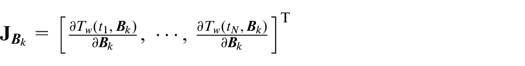
In order to provide the necessary foundation to describe the implementation of the NSALMN optimisation algorithm, a description of the objective function and the algorithm steps should be provided first. In particular, the NSALMN algorithm employs an iterative procedure to minimise the least squares objective function, which depends on the unknown parameters vector
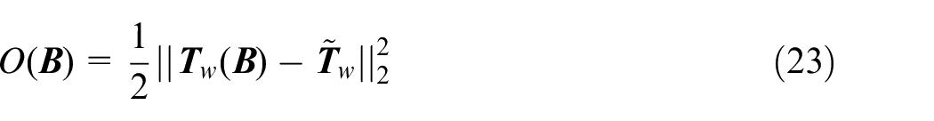
where
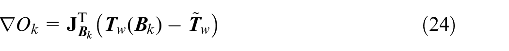
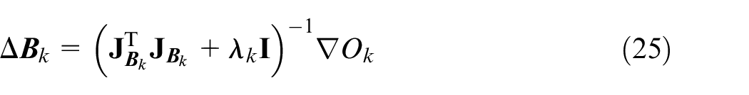
where
The developed method for the solution of the inverse crankshaft dynamics problem employs the NSALMN algorithm. The flowchart of this method that includes the method steps and order of operations is depicted in Figure 3. The method is initiated by providing the following input: (a) an accurate estimate for the initial values of the unknown parameters vector
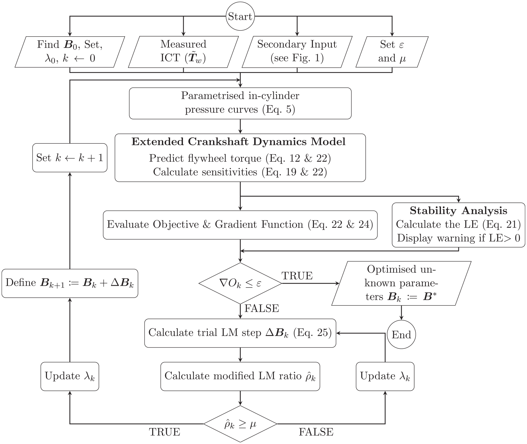
Flowchart of the developed method to solve the inverse problem.
The method then proceeds to the calculation of the in-cylinders pressure variations (for one engine revolution) by employing equation (5), based on the unknown parameters vector
In tandem with the calculation of the objective function and its gradient, the stability analysis is also performed. It should be noted that this is not an original part of the NSALMN algorithm, however it is incorporated as part of the developed inverse problem method. In specific, by using the sensitivity equations calculated from the extended model and equation (21), all of the Lyapunov Exponents (LEs) are calculated corresponding to each one of the sensitivities with respect to the initial conditions
A modified LM ratio
Case studies design
A series of case studies are designed in this study to allow for the testing of the developed method to solve the crankshaft dynamics inverse problem under ideal and realistic operating conditions. However, prior to listing all the case studies, it should be noted that the direct model is employed to provide the mock up ICT data, which are used as input to the inverse problem method. In specific, the direct model simulates the measured ICT by using as input the in-cylinder pressure for each engine cylinder, in accordance to the conditions dictated from each case study, hereinafter referred to as the measured in-cylinder pressures. Thus, the simulated ICT measurement is utilised as the input of the inverse problem method, which is in turn validated by using the method’s output (i.e. the optimised unknown in-cylinder pressure parameters) to reconstruct the in-cylinder pressure diagrams and compare them with the in-cylinder pressures used as input to the direct model. In addition, the inverse problem method performance is evaluated by utilising the following Key Performance Indicators (KPIs):
Number of successful iterations.
Ratio of number of failed to successful iterations.
Method execution time.
Average error and standard deviation between the reconstructed in-cylinder pressure diagrams and the direct model in-cylinder pressure input, as a percentage of the average peak pressure.
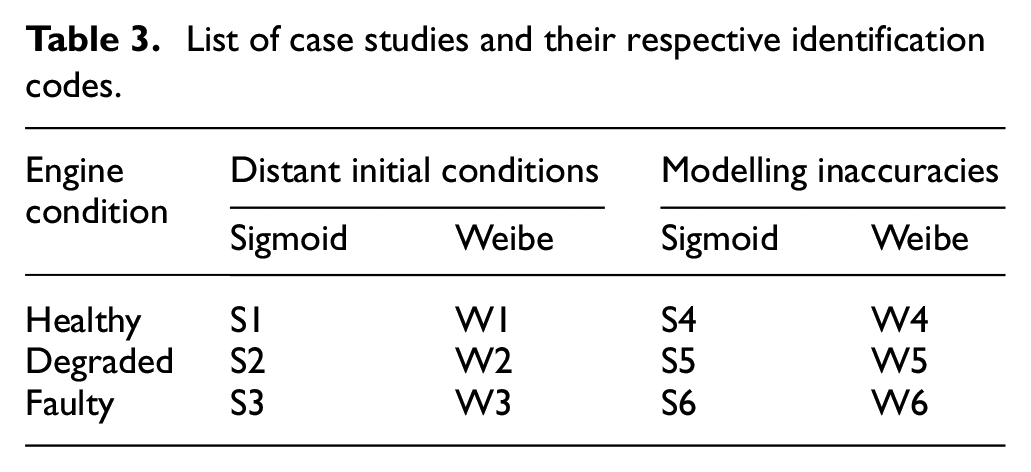
To test the performance of the developed inverse problem method, the designed case studies are classified under the following two main categories: (a) modelling inaccuracies and (b) distant initial conditions. For each of these two main categories, the inverse problem method is tested for the three subcategories of healthy, degraded and faulty engine conditions. Finally, for each subcategory, the extended model is employed using either the sigmoid or Weibe functions to facilitate a comparison in the performance of the inverse problem method. All the case studies are performed for the 100% engine load and are summarised in Table 3.
List of case studies and their respective identification codes.
For the case studies involved in the distant initial conditions category, the initial conditions of the unknown parameters vector
For the case studies corresponding to the modelling inaccuracies category, the mock up ICT is simulated using the direct model, which employs an accurate coefficients matrix engine friction submodel. The latter models the engine friction by using manufacturer-tuned coefficients proportional to the DOF angular speed, instead of a less accurate constant engine friction submodel which is employed by the extended model in the inverse problem method (the specific details for both friction submodels are reported in Tsitsilonis et al. 43 ). By employing different friction submodels, discrepancies in the modelling are purposely introduced. This emulates a realistic scenario, where the physical system (simulated by the direct model with the coefficients matrix engine friction submodel) is not perfectly represented by the extended model (employed by the inverse problem method), which utilises the simplistic constant engine friction submodel. The latter introduces a non-zero residual problem, which can potentially pose additional challenges for the accurate prediction of the in-cylinder pressure. Finally, the modelling inaccuracy is chosen to be introduced in the engine friction rather than in other parts of the engine model, since this part is a very frequent source of errors in dynamic engine modelling. 63
Regarding the first subcategory of healthy engine conditions, the direct model simulation runs are performed by using as input the same in-cylinder pressure for all cylinders. The initial in-cylinder pressure function parameters are determined by performing a best fit of the in-cylinder pressure equation with the measured in-cylinder pressure data at 100% MCR reported in Guerrero and Jiménez-Espadafor 31 for the case of the reference system. This indicates that there are no discrepancies in the condition of each cylinder, and thus the engine is assumed to be in as-healthy-as-new condition.
The degraded engine conditions are simulated by using a random number generator to change the parameters of the healthy in-cylinder pressure functions for each cylinder. In specific, changing the in-cylinder pressure function parameters with respect to the healthy conditions results in subtle alterations in the shape of each individual in-cylinder pressure diagram, thus simulating the degraded conditions for all engine cylinders. As a result, the derived in-cylinder pressure function parameters are employed to generate the degraded in-cylinder pressure diagrams, which are used as input to the direct model for deriving the mock up ICT measurement. To derive the model parameters for engine degraded conditions, a uniform distribution was employed to generate values varying within a range of


where
Finally, the faulty engine conditions are simulated by introducing a complete misfire on the first engine cylinder, whilst the other cylinders have the in-cylinder pressures corresponding to the degraded engine conditions at 100% MCR. It should be noted that misfire events can be identified easily by monitoring the exhaust gas temperatures of each cylinder. However, in this study, the misfire is used as an extreme scenario to test the capabilities and verify the robustness of the developed in-cylinder pressure prediction method.
Results and discussion
Case studies KPIs
Having tested the inverse problem method for all the case studies listed in Table 3, it was deduced that the method was successfully converged for all case studies, and the involved stability analysis did not indicate at any instance the potential occurrence of a chaotic behaviour. Therefore, the performance of the inverse problem method can be analysed holistically for every case study in accordance to the KPIs introduced in Section Case studies design, the obtained results of which are presented in Figure 4. Specific representative case studies were selected to be analysed in detail as presented below in this Section.
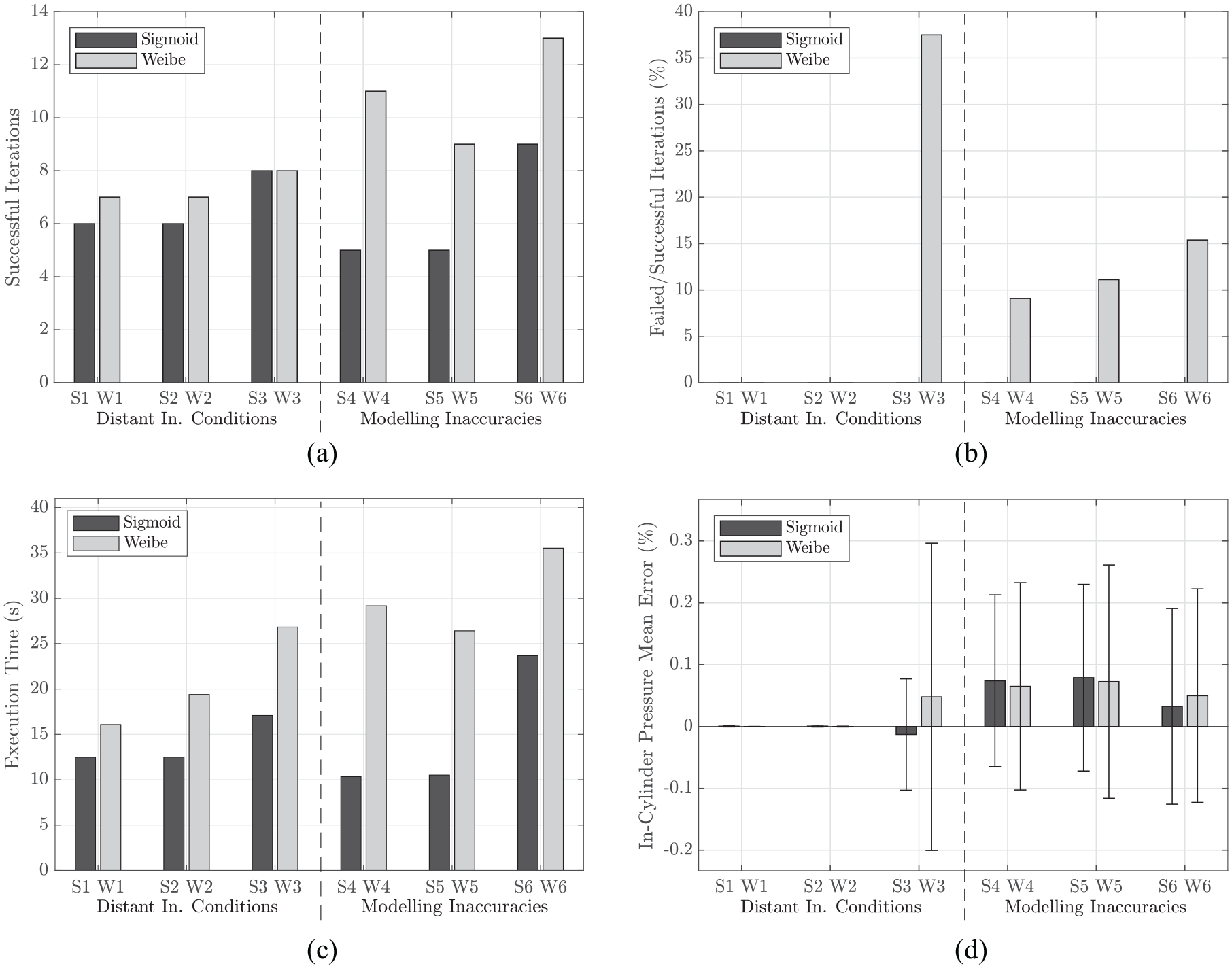
(a) Successful iterations of inverse problem method, (b) failed iterations as a percentage of the successful iterations of the inverse problem method, (c) execution time of inverse problem method and (d) mean pressure error of predicted in-cylinder pressure by the inverse problem method as a percentage of the mean peak pressure (the error bars refer to the error standard deviation).
Firstly, the performance of the inverse problem method employing the Weibe and sigmoid functions is compared. As shown in Figure 4(a), when the Weibe function is employed as compared to the sigmoid function, approximately three additional successful iterations are required on average to achieve convergence, except for cases S3 and W3, where the same number of successful iterations takes place for both functions. Furthermore, as shown in Figure 4(b), failed iterations are observed only for cases W3–W6, which correspond the Weibe function, and range from 9% to 38% of the successful iterations number. In contrast, for cases corresponding to the sigmoid function, no failed iterations take place. Hence, it is deduced that the Weibe function is more computationally demanding, due to the additional parameter that it introduces for each cylinder, which is also a highly nonlinear one. This is confirmed from the results presented in Figure 4(c), where the inverse problem method execution time is consistently greater for all case studies employing the Weibe function, compared to the respective results for the case studies employing the sigmoid function. Regarding the accuracy of the inverse problem method, as shown in Figure 4(d), the mean pressure error does not indicate a specific trend, however the error standard deviations are slightly smaller for the case of the sigmoid function by an average of 0.04% for all case studies. This implies that the error does not depend on whether a Weibe or a sigmoid function is used as interpolating function. In addition, the maximum observed error is 0.3%, which indicated that the developed method is quite accurate in predicting the in-cylinder pressure diagrams.
The two main categories of the distant initial conditions and the modelling inaccuracies are compared (corresponding to the first and second columns in Table 3, i.e. case studies S1–S3 and W1–W3 vs S4–S6 and W4–W6). As shown in Figure 4(a), the distant initial conditions as compared to the modelling inaccuracies case studies take on average three additional iterations for the Weibe, or one less successful iteration for the sigmoid function. In addition, as shown in Figure 4(b), with the exception of case study W3, the failed iterations correspond entirely to the modelling inaccuracies case studies with the Weibe function. Furthermore, as expected the method execution time directly correlates with the total number of successful and failed iterations as shown in Figure 4(c). Overall, this indicates that for the distant initial conditions as compared to the modelling inaccuracies case studies, the inverse problem method performs faster by an average of 9.7 s for the Weibe function, or slower by an average of 0.5 s for the sigmoid function.
Most importantly, as shown in Figure 4(d), for the case of the distant initial conditions, despite case studies S3 and W3, which are discussed in detail below, the in-cylinder pressure mean error is almost negligible. This is expected as a zero-residual objective function has been formulated. In contrast, for all the case studies corresponding to the modelling inaccuracies, the in-cylinder pressure mean error only slightly increases (by an average of 0.07%) and a standard deviation of 0.25% of the mean maximum pressure, which although small, is significantly greater as compared to the distant initial conditions case studies. This indicates that from all the case studies, the ones corresponding to the modelling inaccuracies can result to the largest in-cylinder pressure mean errors. However, the error is still sufficiently small, and this is a favourable characteristic of the inverse problem, since a small effect on the in-cylinder pressure error is caused even for considerable modelling inaccuracies of the engine friction model.
The three subcategories of the healthy, degraded and faulty engine conditions are compared. Regarding the Weibe and sigmoid functions for both the modelling inaccuracies and distant initial conditions case studies, as shown in Figure 4(a) and (b), the faulty engine conditions (S3, W3 and S6, W6) seem to require the greatest number of iterations to achieve convergence; 13 and 8, respectively. Special notice is taken for the case study W3 due to the large number of failed iterations, which approaches 38% of the total successful iterations, as shown in Figure 4(b), as well as the largest mean in-cylinder pressure error standard deviation shown in Figure 4(d). In addition, case study S3 also exhibits considerably larger mean in-cylinder pressure error than the other two case studies in its respective category, which correspond to the distant initial conditions using the sigmoid function. This implies that the faulty engine condition represented with a misfire on cylinder no. 1, is the most computationally intensive case study. This is attributed to the fact that the initial conditions, which are always provided as those of a healthy engine with identical in-cylinder pressures for all cylinders, lie further from the objective function minimum. However, by examining the healthy and degraded engine conditions for both the Weibe and sigmoid functions, small or no differences are observed in the total number of successful or failed iterations respectively. Moreover, the inverse problem method appears to be the fastest as shown in Figure 4(c), when compared to the faulty engine conditions, by an average of 8.9 and 8.2 s for the Weibe and sigmoid functions, respectively. This implies that the developed method behaves very similarly, between the healthy and degraded engine conditions as the objective function minima between these two engine conditions are fairly similar despite the changes of the in-cylinder pressure parameters from cylinder to cylinder for the degraded engine conditions.
Individual case studies analysis
Following the KPIs analysis presented in the preceding section, a more specific discussion is provided for two representative case studies as explained below. Case study W3 is considered for detailed analysis due to the following reasons: (a) it exhibits the largest in-cylinder pressure error standard deviation of 0.25% as presented in Figure 4(d)); (b) it has by far the largest percentage of failed iterations, which contributes in exhibiting the third slowest execution time of 24.5 s (Figure 4(b) and (c), respectively); and (c) it is amongst the most complex case studies, as it employs the highly non-linear Weibe function and the engine experiences faulty conditions (deviations in the in-cylinder pressures of each individual cylinder and a misfire on cylinder no. 1).
Furthermore, case study S4 will also be analysed as justified in the following. It is amongst the fastest performing case studies with an execution time 10.9 s with no failed iterations (Figure 4(b) and (c), respectively). Moreover, it employs the sigmoid function, it corresponds to the engine healthy engine conditions and belongs to the case studies category of the modelling inaccuracies. Therefore, case study S4 is by far the one with the greatest difference in setup from case study W3. Both case studies S4 and W3 demonstrate interesting characteristics among the entire spectrum of the investigated case studies.
Starting with the case study S4, the engine ICT variations at the flywheel for one engine revolution are shown in Figure 5(a) (this figure shows both the ICT provided as input to and the ICT predicted by the inverse problem method). The ICT counter-intuitively exhibits five peaks instead of the expected 10 peaks, which would correspond to 10 engine cylinders. This is due to the non-linearities introduced primarily by the large reciprocating and rotating masses of the engine’s piston assembly.43,66 It is observed that the measured ICT data sufficiently match the ICT from the extended model deployed within the inverse problem method.
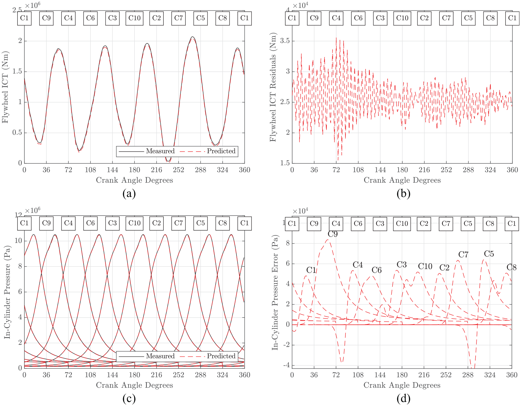
(a) Measured ICT data simulated by the direct model, and predicted ICT by the inverse problem method at the final iteration, for case study S4, (b) flywheel ICT residuals between measured and predicted flywheel torque at final iteration of the inverse problem method, for case study S4, (c) measured and predicted in-cylinder pressure by the inverse problem method, for case study S4 and (d) error between the simulated and predicted in-cylinder pressure by the inverse problem method, for case study S4.
As shown in Figure 5(b), the residuals between these ICT variations fluctuate at approximately two orders of magnitude less than the measured ICT data, which demonstrates a very small difference. In specific, this difference is also positive, which signifies that the measured ICT data is greater than the predicted ICT, which is derived by using the extended direct model (called by the inverse problem method) employing the simplified constant engine friction model. This results from how the inverse problem optimisation algorithm approaches the objective function minimum, which partially depends on the provided initial conditions. Furthermore, the torque residuals exhibit a high frequency fluctuation, which indicates that there are intrinsic physical differences between the measured and predicted ICT. However, this frequency is higher than the 40th engine order, which for the case where a torque metre is used to obtain the measured ICT data (in contrast to this study where a simulation is performed) can be considered as noise that needs to be filtered.
Figure 5(c) presents the predicted pressure diagrams by the inverse problem method (by employing the extended direct model) along with the pressure diagrams (fitted from the measured pressure reported in Guerrero and Jiménez-Espadafor 31 for the engine operation at 100% load), which were used as input by the direct model. As this case study corresponds to healthy engine conditions, the measured pressure diagrams of each engine cylinder are identical and shifted in the crank angle axis by each cylinder phase angle. Most importantly as shown in Figure 5(d), the predicted in-cylinder pressure diagrams exhibit a very small error compared to the measured in-cylinder pressure diagrams (which were provided as input in the direct model to simulate the ICT data), reaching a maximum of 0.8 bar for cylinder no. 9. As also mentioned in the preceding paragraphs, these obtained results confirm that the modelling inaccuracies in the engine friction sumbodel do not result in significant errors in the predicted in-cylinder pressure. Similarly to the ICT residuals, the in-cylinder pressure error is primarily positive, which indicates that the simulated in-cylinder pressure is, for most crank angle positions, greater than the predicted in-cylinder pressure. Furthermore, the pressure error reaches its greatest values for each individual cylinder after the respective cylinder’s TDC, near the in-cylinder peak pressure, with the maximum error incurred in cylinder no. 9. This takes place because changes in the in-cylinder pressure function unknown parameters affect the shape of the in-cylinder pressure curve mostly near its peak, which occurs close to the TDC location. Hence the error can become more pronounced at the TDC location.
For the case study W3 that corresponds to faulty engine conditions with a misfire on cylinder No. 1, degraded conditions of all the other cylinders and use of Weibe function, the ICT predicted by the inverse problem method as well as the ICT provided as input to the inverse problem method are shown in Figure 6(a). It is observed that the ICT exhibits four peaks (instead of five as discussed for the case study S4). In specific, the ICT peak that is located after the cylinder no. 9 TDC is not present when a misfire on cylinder no. 1 occurs, which demonstrates that the effect of the misfire on the flywheel ICT lags the actual misfire event by approximately 36° crank angle. This occurs as a result of the crankshaft’s flexibility, hence the changes in torque due to the different forces exerted in each piston do not get transmitted instantly to the flywheel.31,43 In this case study as shown in Figure 6(b), since no modelling inaccuracies are introduced, the ICT residuals are three orders of magnitude smaller than the measured ICT, which is also one order of magnitude less than those for case study S4 discussed above. Furthermore, a similar high frequency fluctuation is not visible as it was found for the case study S4, which is attributed to the fact that no modelling inaccuracies are introduced for this case study. In addition, the average residuals for case studies W3 and S4 have an average value of approximately 0 Nm and
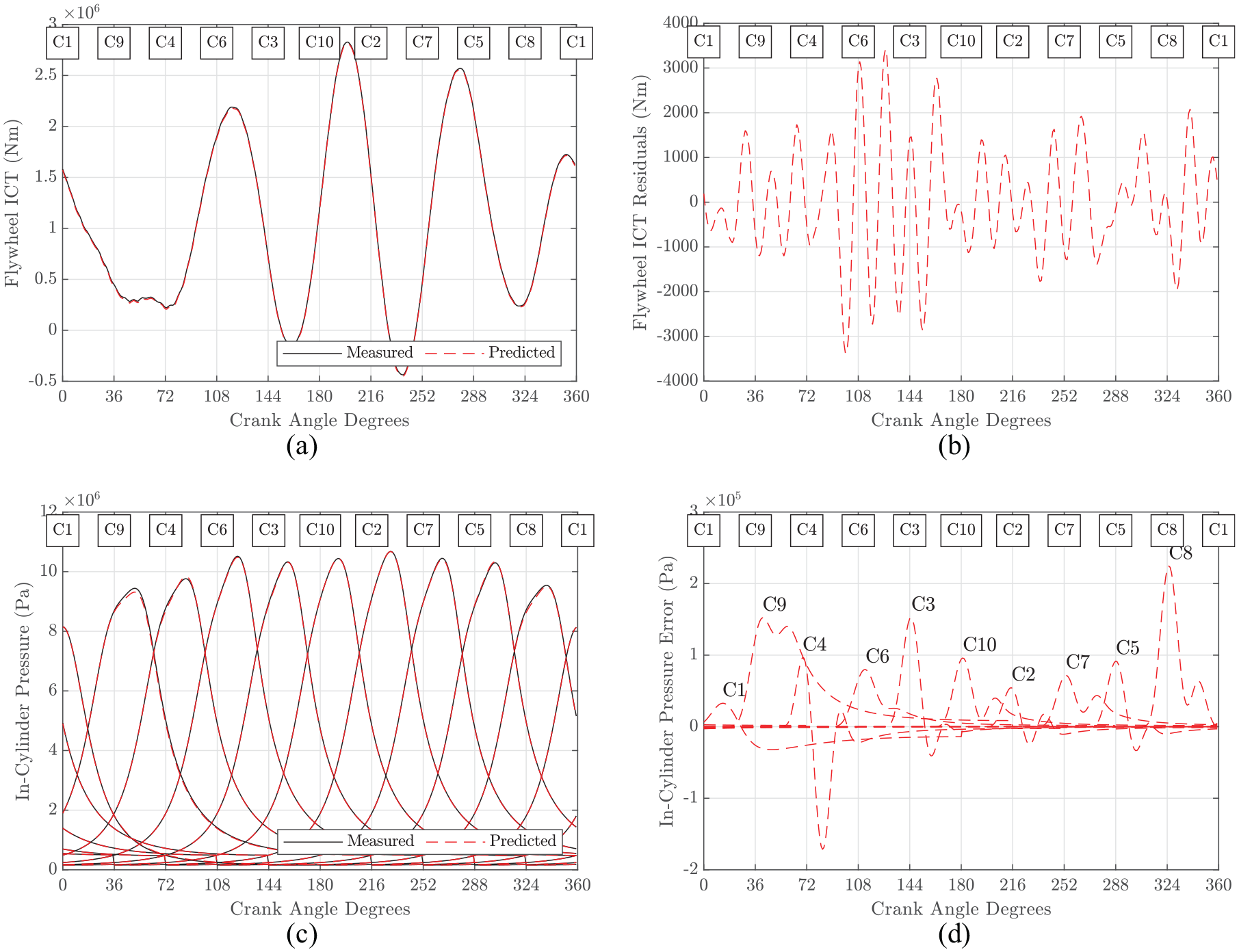
(a) Measured ICT data simulated by the direct model, and predicted ICT by the inverse problem method at the final iteration, for case study W3, (b) flywheel ICT residuals between measured and predicted flywheel torque at final iteration of the inverse problem method, for case study W3, (c) measured and predicted in-cylinder pressure by the inverse problem method, for case study W3 and (d) error between the simulated and predicted in-cylinder pressure by the inverse problem method, for case study W3.
Moreover, as shown in Figure 6(c), the measured in-cylinder pressure variations almost coincide with the predicted ones. However, as shown in Figure 6(d), the in-cylinder pressure error is significantly greater by one order of magnitude compared to the respective errors observed in the case study S4. This error is still acceptable, however, since the peak pressure values reach an average of approximately 100 bar for the cylinders no. 2–10, the maximum pressure error reaches a value of around 2.2 bar, which occurs for cylinder no. 8 close to its TDC. The much larger magnitudes for the in-cylinder pressure errors obtained in the case study W3 are attributed to the significantly greater non-linearities of the Weibe function as compared to the sigmoid function.
These non-linearities introduce radical topological changes in the shape of the objective function, which especially when providing initial conditions further from its minimum, can pose a challenge to the optimisation algorithm’s convergence. This is demonstrated by the visualised two-dimensional subdomains of the objective function for the sigmoid and Wiebe functions shown in Figure 7. In specific, for the case of the sigmoid function (Figure 7(a)), the objective function contours exhibit a mildly elliptical shape, which greatly simplifies the task of the optimisation algorithm. In contrast, for the case of the Weibe function (Figure 7(b)), the objective function contours form a narrow canyon shape that contains a number of local minima, which can potentially pose challenges for the optimisation algorithm. As observed from the presented path of the optimisation algorithm, it gets trapped close to the local minimum within the narrow canyon. The algorithm subsequently resets and the optimisation process recommences from the closest point outside the canyon, where the objective function slope is more pronounced and thus, convergence can be achieved. Hence, when the Weibe function is employed, the optimisation algorithm has to follow a more complex path to reach its minimum, and as a result, its efficiency and performance is not as consistent. However despite the above, as shown from both Figure 6(a) and (b), the cylinder no. 1 with misfiring was identified correctly based on the predicted in-cylinder pressure by the inverse problem method and with the best accuracy, as the prediction exhibits the smallest maximum pressure error compared to all other cylinders.
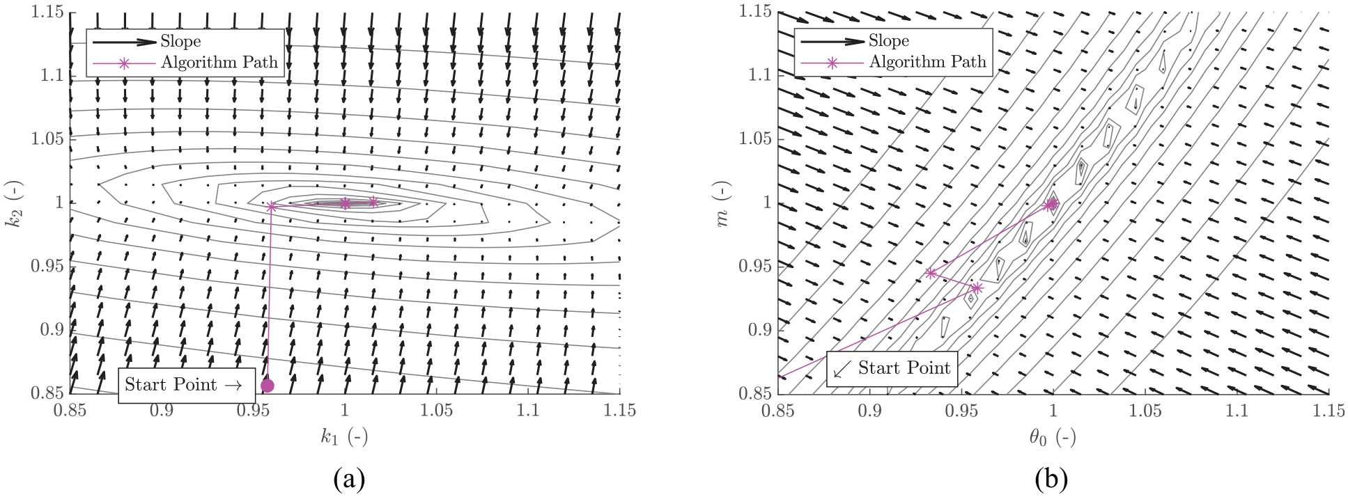
(a) Two-dimensional subdomain of the objective function by varying the unknown parameters
The inverse problem method was also tested for two other engine loads of 55% and 70%. These tests were performed by using the same case studies as above, with the corresponding changes made in their set up in order to accommodate for the different engine loads being tested. The results obtained were similar to the ones described above for 100% load.
In addition, from the preceding analysis, it was observed that the developed inverse model succeeded in identifying the sigmoid and Weibe functions parameters (three and four parameters per cylinder, respectively), and as a result the in-cylinder pressure diagrams for all the investigated case studies. In this study, the ICT was provided with a resolution of one data sample per degree crank angle. Therefore, it is concluded that the inverse model is characterised as identifiable 67 for both the sigmoid and Weibe functions, provided that the ICT signal resolution is at least one sample per degree crank angle.
Sensitivity analysis
The results from the S4 and W3 case studies can be correlated to specific features of the flywheel torque sensitivities with respect to the unknown in-cylinder pressure parameters for improving the understanding of the inverse problem. As the sensitivities exhibit a consistent oscillatory behaviour throughout a complete crankshaft revolution, the sensitivity analysis herein was conducted by using the Euclidean norm of all the sensitivities. The respective results are presented in Figure 8.
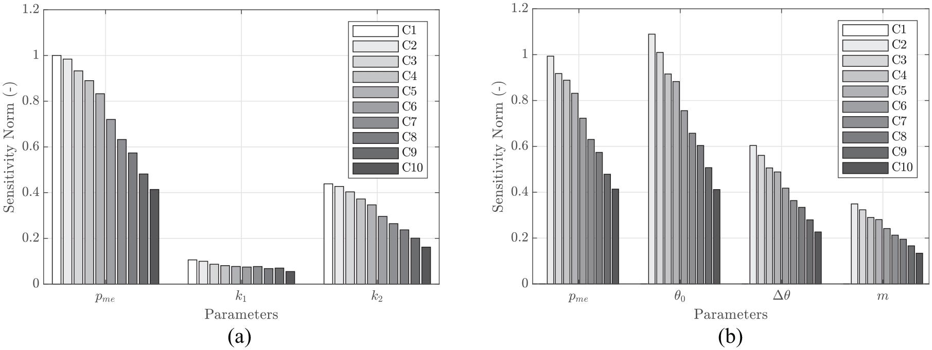
(a) Normalised sensitivities Euclidean norm of the unknown parameters with respect to the flywheel torque, for case study S4 and (b) normalised sensitivities Euclidean norm of the unknown parameters with respect to the flywheel torque, for case study W3.
By considering the sensitivities corresponding to parameters
Furthermore, by comparing the parameter sensitivities across individual cylinders, it is observed from Figure 8(a) and (b) that the cylinder further away from the flywheel exhibits larger sensitivity norm for all parameters. This implies that the unknown parameters of the cylinders further from the flywheel exhibit a greater impact on the flywheel torque calculation. As a result, the engine ICT is less sensitive to changes in the parameters of the cylinders closest to the flywheel.
In addition, as observed by the results presented in Figure 7, due to the misfire on cylinder no. 1, the sensitivities of all the unknown parameters are zero. This is due to the fact that combustion does not take place when a misfire occurs. As a result, the unknown parameters, which relate to the respective cylinder’s combustion, do not contribute to the engine’s ICT. Finally, the sensitivity norms corresponding to parameter
Conclusions
This study developed a novel method to solve the inverse problem of determining the in-cylinder pressure, based on the measurement of the crankshaft ICT. This method was based on the IVP technique and employed an optimisation algorithm along with a lumped parameter crankshaft dynamics model. The applicability of the method was tested for various cases including healthy, degraded and faulty engine conditions, as well as considering the lack of in-cylinder pressure data, and modelling inaccuracies. It was found that this method accurately predicted the in-cylinder pressure with a maximum error of less than 0.5% from the respective measured values.
In specific, from the two interpolating functions that were tested, the Weibe function performed the slowest response by an average of 11.2 s as compared to the sigmoid. However, there was no significant effect to the in-cylinder pressure error. As a result, it is recommended to use the Weibe interpolating function, since despite the increased computational burden, it is able to model the combustion more accurately, due to the employed additional parameter, compared to the sigmoid function. Furthermore, the inverse problem method demonstrated its robustness when tested for both distant initial conditions and modelling inaccuracies, with a slightly errors on the predicted in-cylinder pressure by 0.07% on average for the latter case. Testing at healthy, degraded and faulty engine conditions provided lower execution time was slower for the degraded and healthy engine conditions by an average of 8.5 s as compared to the healthy conditions, whereas no significant changes were observed for the in-cylinder pressure error.
Further insight into the inverse problem of estimating the in-cylinder pressures by utilising the engine ICT at the flywheel was also obtained, by considering the individual sensitivities of the unknown in-cylinder pressure parameters. In specific, the cylinders further from the flywheel exhibited smaller sensitivities and thus have a smaller impact on the engine ICT. In addition, the parameters
Therefore, it can be concluded that the developed method for predicting the in-cylinder pressure based on the engine ICT measurement exhibited adequate performance. This method implementation has the potential for a significant change in the maritime industry norm by employing a permanently installed shaft torque metre sensor with the capability of obtaining higher sample rates, thus replacing the use of external in-cylinder pressure measurement kits, or expensive multi-sensor continuous pressure monitoring systems. This will allow the continuous and non-intrusive monitoring of the in-cylinder pressure without requiring extensive retrofitting to deploy multiple sensor networks.
Future studies will include testing of the developed method by using the ICT data scheduled to be obtained from large marine four-stroke and two-stroke engines. Further development will include modifying the method to be implemented in on-line applications, as well as expanding the method to integrate decision support capabilities.
Footnotes
Acknowledgements
The opinions expressed herein are those of the authors and should not be construed to reflect the views of DNV AS, RCCL and Innovate UK.
Declaration of conflicting interests
The author(s) declared no potential conflicts of interest with respect to the research, authorship, and/or publication of this article.
Funding
The author(s) disclosed receipt of the following financial support for the research, authorship, and/or publication of this article: The authors from MSRC greatly acknowledge the funding from DNV AS and RCCL for the MSRC establishment and operation. The authors also gratefully acknowledge the financial support of Innovate UK, through the Knowledge Transfer Partnership project (project number 11577), for the work reported in this article.