Sage Journals: Discover world-class research

Abstract

This study proposed ordered probit models as a methodology to verify the male-taller norm and the male-not-too-tall norm while controlling for other factors. This study confirmed the prevalence of the male-taller and the male-not-too-tall norms in Taiwan. The frequency of the height difference between a husband and wife within the range of 5–15 cm was higher than what would be expected by chance. This range in Taiwan was smaller than the range in the United Kingdom, which may imply that there are preferred height differences between couples that vary across populations.

Keywords

height male-taller norm male-not-too-tall norm assortative mating ordered probit model Taiwan

Studies on desired partners have shown that an ideal partner for a male is shorter than himself, whereas for a female, an ideal partner is taller than herself (Buss & Barnes, 1986; Fink, Neave, Brewer, & Pawlowski, 2007; Higgins, Zheng, Liu, & Sun, 2002; Pierce, 1996; Salska et al., 2008; Yancey & Emerson, 2016). This rule has been called the “male-taller” norm (Gillis & Avis, 1980), and women are more likely to comply with the male-taller norm than men (Stulp, Buunk, & Pollet, 2013). In studies on personal advertisements, Pawlowski and Koziel (2002) and Campos et al. (2002) found that the response rate or hit rate for tall males was greater, but for tall females, it was lower. In personal advertisements, females usually seek a taller partner (Koestner & Wheller, 1988). Shepperd and Strathman (1989) reported that females rated taller males as being more attractive. Taller males had also dated more frequently than their counterparts. In the marriage market, a male’s height is valued by females.

Male physical contests for mates are rare in modern societies. Yet, male height still matters in female mate selection. Two possible reasons explain why modern women prefer tall men. First, as evolutionary psychology suggests, modern female height preferences might be inherited from our ancestors (Judge & Cable, 2004; Murray & Schmitz, 2011). Namely, tall males are perceived to be more attractive. Secondly, studies have shown that male height is positively associated with educational attainment (Cinnirella, Piopiunik, & Winter, 2011; Magnusson, Rasmussen, & Gyllensten, 2006; Meyer & Selmer, 1999; Silventionen et al., 1999; Szklarska, Koziel, Bielicki, & Malina, 2007), income (Böckerman & Vainiomäki, 2013; Case & Paxson, 2008; Kortt & Leigh, 2010; Lundborg, Nystedt, & Rooth, 2014; Persico, Postlewaite, & Silverman, 2004), leadership (Blaker et al., 2013; Murray & Schmitz, 2011; Stulp, Buunk, Verhulst, & Pollet, 2013), and status (Case & Paxson, 2008; Heineck, 2005; Komlos & Kriwy, 2002; Krzyżanowska & Mascie-Taylor, 2011; Silventoinen, Lahelma, Lundberg, & Rahkonen, 2001). Specifically, for the first explanation, evolutionary psychology argues that women are born with the perception that tall men are more attractive than short men. The second explanation indicates that men’s height is positively correlated with resource access.

The male-taller norm is not universally true, in particular not in some indigenous populations that have been isolated from modernization. On the one hand, Sear and Marlowe (2009) found that mate selection for actual couples is random with respect to height in the Hadza, a hunter-gatherer population living in Tanzania. Sorokowski and Sorokowska (2012) reached the same conclusion with regard to Yali populations, a traditional ethnic group living in the mountains of Papua, Indonesia. Sorokowski and Butovskaya found that both sexes in Datoga, a tribe living in Tanzania, prefer their partners to be either much taller or much shorter than themselves. The mate selection in these populations violates the male-taller norm. On the other hand, Sorokowski et al. (2015) did find the male-taller preference in some indigenous populations, such as the Hadza and the Tsimané. The Tsimané are a native Amazonian society of farmer foragers in the area of Beni in northern Bolivia, while the Hadza were also investigated by Sear and Marlowe (2009) as mentioned above. Becker, Touraille, Froment, Heyer, and Courtiol (2012) found that the male-taller norm even prevailed in Baka pygmies in central Cameroon.

Furthermore, although the male-taller norm prevails in Western countries, people prefer the height difference between a husband and wife to be within a certain range (Courtiol, Raymond, Godelle, & Ferdy, 2010; Fink et al., 2007; Pawlowski, 2003; Salska et al., 2008; Stulp, Buunk, Pollet, Nettle, & Verhulst, 2013; Stulp, Mills, Pollet, & Barrett, 2014; Yancey & Emerson, 2016). This preference is named the “male-not-too-tall” norm. Stulp, Buunk, Pollet, Nettle, and Verhulst (2013) was the first to indicate that the most frequent range of height difference was within 25 cm in the United Kingdom. If the two explanations aforementioned can fully support the male-taller norm, then short women look for the same tall men as tall women do. But this is not what we observed. The incomplete explanation of evolutionary psychology and resource access hypotheses on assortative mating with respect to height implies more hypotheses are needed.

Recently, in addition to the two possible explanations for the male-taller norm, researchers (Salska et al., 2008; Swami et al., 2008; Yancey & Emerson, 2016) have proposed a third possible explanation, a socialization explanation, for the male-taller norm. They argued that the male-taller norm is a reflection of sex-role ideology or sex stereotype because height amounts to dominance. Although the sex-role explanation can be partially covered by the first two explanations, Yancey and Emerson (2016) showed that height preference for a mate should not violate societal expectation. Respondents clearly specified that a great height difference is awkward or weird even though the male-taller norm was met. In other words, when people look for a mate, they prefer a male taller than his coupled female but not too tall.

The purpose of this study was to use Taiwanese data to verify the assortative mating with respect to height: the male-taller and male-not-too-tall norms in Taiwan. This study contributes to the literature on assortative mating with respect to height in three ways. First, most of the existing evidence of the assortative mating with respect to height are from Western populations (Krzyżanowska, Mascie-Taylor, & Thalabard, 2015; Sear, 2010). The conclusion of this study provides evidence from Eastern population. Second, the conclusions of the assortative mating with respect to height are usually challenged by the possibility that the observed assortative mating with respect to height is due to characteristics other than height, say education (Stulp, Buunk, Pollet, et al., 2013). This study employed an ordered probit model to verify the male-taller and the male-not-too-tall norm, while controlling for other characterisitcs. Third, using a sample from the United Kingdom, Stulp, Buunk, Pollet, et al. (2013) found that couples where the male partner was taller than the female partner within 25 cm occurred at a higher frequency in actual couples than that expected by chance. If the male-not-too-tall norm does prevail in a society, the most frequent height difference between a couple observed might vary with societies. It would be interesting to see whether the most frequent height difference between a couple will change for Eastern population, and what the implications are if such difference is observed.

Material and Method

Sample

The data were from the Elementary School Children’s Nutrition and Health Survey (ESCNHS) in Taiwan 2001–2002, financially supported by the Ministry of Health and Welfare and compiled by Academia Sinica in 2001 and 2002. The purpose of this survey was to investigate elementary students’ nutrition and health status. This survey also asked students’ parents to report their heights. To date in Taiwan, this is a rare data set simultaneously documenting the wife’s and the husband’s height. The ESCNHS is unique for the purpose of this study. In all, 3,069 students were drawn by stratified random sampling from the whole nation, and 2,419 students and their families completed the questionnaire. After deleting single parent and observations without height, age, educational attainment, and family income, 1,344 observations remained for husband and wife samples. This is the studied sample.

The ESCNHS separatively asked a child’s father and mother their family income: “Taking all income sources into account, on average, how much is your monthly family income?” The answer is categorized to (1) less than 10,000, (2) 10,000 –20,000, (3) 20,000–30,000,…, (15) 140,000–150,000; (16) more than 150,000 New Taiwan dollars, (17) uncertain income, and (18) no income. The other categories are “don’t know” and “refused to answer.” The middle values from Categories (2) to (15) are used to be their family income. The income proxy for Categories (1) and (16) are 5,000 and 155,000 New Taiwan dollars, respectively. The amount of income is 0 for uncertain income and no income. If only one spouse reported that the family has income, then this reported income is used as the family income. When both father and mother reported their family income, their average value is taken as their family income.

Educational attainment is recorded in 21 educational categories in the questionnaire. These educational categories are transferred into 11 categories in terms of educational years. For example, diploma of senior high school, vocational senior high school, and army academy senior high school all indicate 9 years of education. The questionnaire contains 7 levels of educational attainment: no education, elementary school, junior high school, senior high school, junior college, college, and postgraduate school. The 21 educational categories includefive other categories that do not finish the middle five educational levels, for example, some years in elementary school. In these cases, respondents who reported studying for some years in certain educational level are assumed finishing half of the number of educational years. As some years in college and graduates of junior college have the same number of educational years, these two categories have the same number of educational years. Consequently, there are 11 categories in terms of educational years. In addition to height, Table 1 presents that average family income and its standard deviation of this data set are 62,619 and 34,099 New Taiwan dollars, respectively. They are respectively about 1,957, and 1,066 U.S. dollars. Husbands’ and wives’ average educational years are 11.7 and 11.2 years, respectively. Their respective standard deviations are 2.86 and 2.71. On average, husbands are older than their wives by about 3 years. The average ages for husbands and wives are, respectively, 40.3 and 37.4, and their standard deviations are 4.83 and 4.64, respectively. The average age of their children is 8.45, and its standard deviation is 1.70 (not shown in Table 1).

Table 1.

Descriptive Statistics by Sex and by Height.

Husband Height (cm)	Husband Height (cm)	Wife Height (cm)	Relative Height	Family Income (New Taiwan Dollars)	Husband Education (Years)	Husband Age (years)	n
Mean	169.4 (5.36)	157.9 (5.03)	1.07 (0.04)	62,619 (34,099)	11.7 (2.86)	40.3 (4.83)	1,344
<160	158.7 (2.50)	154.4 (4.70)	1.03 (0.04)	43,457 (26,156)	10.1 (2.90)	42.9 (5.62)	81
160 < H ≤ 165	163.8 (1.34)	156.8 (4.80)	1.05 (0.03)	54,782 (27,827)	10.9 (2.84)	41.0 (4.88)	252
165 < H ≤ 170	168.6 (1.27)	157.9 (5.02)	1.07 (0.03)	63,282 (32,636)	11.6 (2.84)	40.2 (4.53)	515
170 < H ≤ 175	173.1 (1.39)	158.4 (4.84)	1.09 (0.03)	67,523 (32,452)	12.1 (2.66)	39.8 (4.42)	333
>175	178.3 (2.38)	160.0 (4.91)	1.12 (0.04)	72,147 (32,260)	12.7 (2.44)	39.3 (4.51)	163
r		.23	.61	.22	.24	–.19
p Value		<.001	<.001	<.001	<.001	<.001
Wife height					Wife education	Wife age
Mean					11.2 (2.71)	37.4 (4.64)	1,344
≤150	166.9 (5.27)	148.8 (1.99)	1.1 (0.04)	49,733 (25,954)	10.4 (2.76)	37.7 (5.15)	131
150 < H ≤ 155	168.7 (5.44)	153.7 (1.27)	1.1 (0.04)	60,705 (33,032)	11.0 (2.87)	37.7 (4.82)	298
155 < H ≤ 160	169.4 (5.06)	158.3 (1.39)	1.1 (0.03)	61,984 (30,476)	11.2 (2.58)	37.3 (4.50)	572
160 < H ≤ 165	170.6 (5.49)	162.9 (1.36)	1.0 (0.03)	72,235 (34,168)	11.8 (2.37)	36.8 (4.42)	264
>165	172.1 (4.50)	168.3 (2.02)	1.0 (0.03)	63,671 (33,299)	11.4 (2.77)	37.5 (3.76)	79
r	.23		–.63	.15	.14	–.08
p Value	<.001		<.001	<.001	<.001	.005

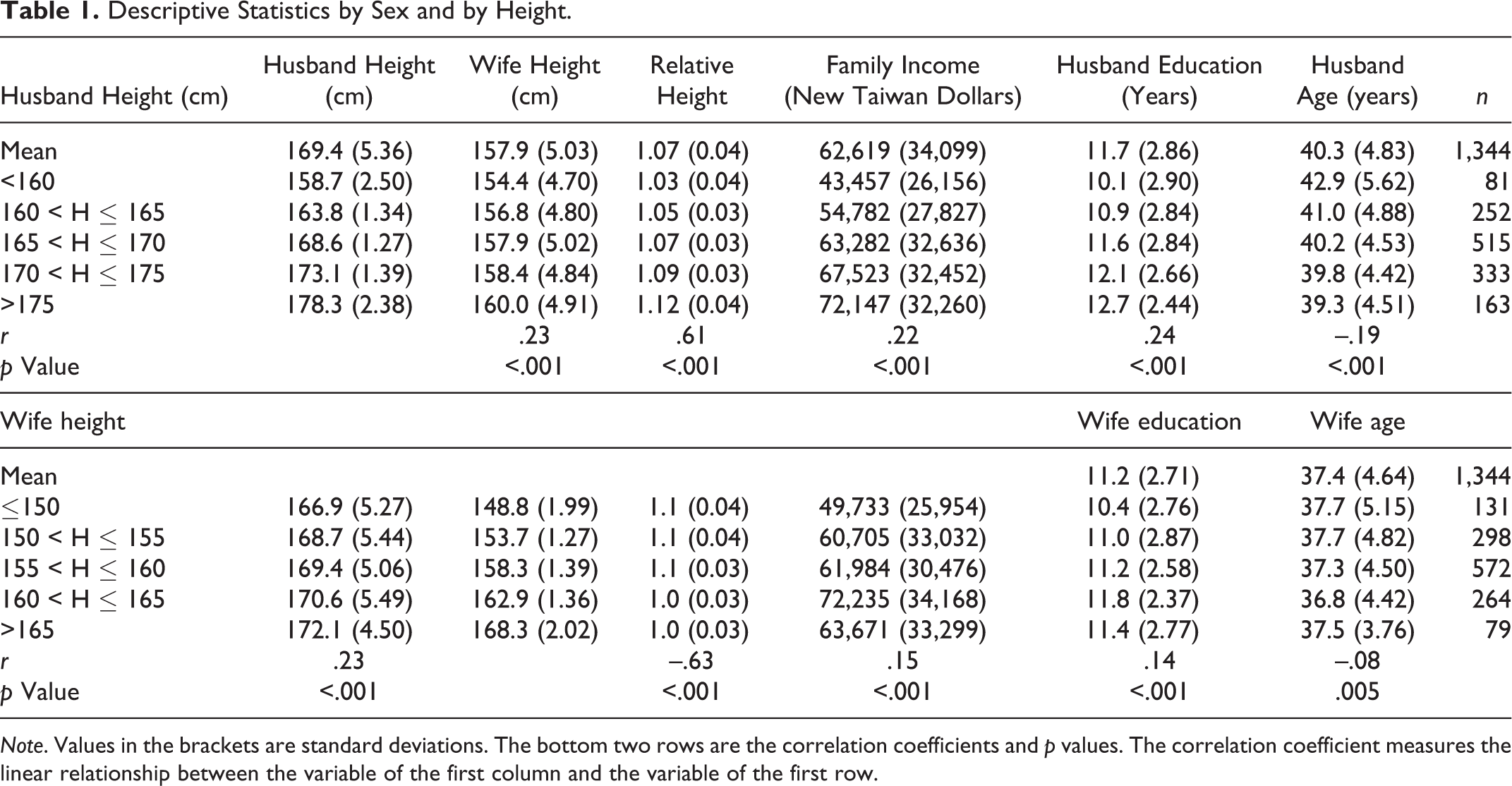
Note. Values in the brackets are standard deviations. The bottom two rows are the correlation coefficients and p values. The correlation coefficient measures the linear relationship between the variable of the first column and the variable of the first row.

Method

Random Simulation

Given the distributions of male and female heights in this sample, this study conducted a random match of men and women. A random simulation was repeatedly run 200 times. A random value X was drawn and was assigned to each husband. In the simulation, the 1,344 wives were not resorted. In all, 1,344 husbands were then resorted according to the magnitude of the drawn random value, and a new set of random matches was obtained. Recall that parents in this sample had children of a similar age meaning that all males and females in this sample can be recoupled in terms of their own ages. In other words, the random simulation will not generate a couple where the husband is aged 25 and a wife is aged 70.

Ordered Probit Model

A woman of a certain height group might be more likely to be married to a man of a certain height group, say 5–15 cm taller than themselves. An ordered probit model is appropriate for this study’s purpose. The dependent variable of an ordered probit model is an ordinal and discrete variable. A continuous height variable can be classified into several categories, as in Table 1. An ordered probit model cannot be successfully conducted when any category of the dependent variable contains a few observations. Because only a small number of husbands were shorter than or equal to 155 cm, the model specifies husbands shorter than or equal to 160 cm as one category. Similarly, wives taller than 170 cm were rare; this category was combined with 166–170 cm. Consequently, there were respectively five height categories for husband’s height and wife’s height as each model’s dependent variable. As spouse height was the explanatory variable, it was classified into five categories. Through this classification, the study could examine which wife height category was more likely to be matched with which husband height category.

The basic model was

y * = x β + ε,

where y* is a latent variable, x is a matrix of independent variables, β is the coefficient vector, and ε is the random error term and obeys a standard normal distribution. Height was divided into five groups, and each group was assigned a new discrete value y. The shortest group was rescaled to be 0, the tallest group was 4, and the groups were rescaled to be 0–4 in order. That is,

y = 0 if y * \leq 0, i.e., ε \leq - β x,

y = 1 if 0 \leq y * < μ_{1}, i.e., - β x < ε \leq μ_{1} - β x,

y = 2 {if μ}_{1} \leq y * < μ_{2}, i.e {., μ}_{1} - β x < ε \leq μ_{2} - β x,

y = 3 {if μ}_{2} \leq y * < μ_{3}, i.e {., μ}_{2} - β x < ε \leq μ_{3} - β x, and

y = 4 {if μ}_{3} \leq y *, i.e {., μ}_{3} - β x \leq ε,

where μ₁ to μ₃ are thresholds of each group and are simultaneously estimated with β. The probability of each group is as follows:

Prob (y =0) = Φ (- β x) = 1 - Φ (β x),

Prob (y = 1) = Φ (μ_{1} - β x) - Φ (- β x),

Prob (y = 2) = Φ (μ_{2} - β x) - Φ (μ_{1} - β x),

Prob (y = 3) = Φ (μ_{3} - β x) - Φ (μ_{2} - β x), and

Prob (y = 4) = 1 - Φ (μ_{3} - β x),

where Φ is the cumulative of distribution function of the standard normal distribution. The marginal probability of an independent variable can be derived as below.

\partial Prob (y = 0) / \partial x = - φ (- β x) β,

\partial Prob (y = 1) / \partial x = [- φ (μ_{1} - β x) + φ (- β x)] β,

\partial Prob (y = 2) / \partial x = [- φ (μ_{2} - β x) + φ (μ_{1} - β x)] β,

\partial Prob (y = 3) / \partial x = [- φ (μ_{3} - β x) + φ (μ_{2} - β x)] β, and

\partial Prob (y = 4) / \partial x = φ (μ_{3} - β x) β,

where φ is the probability density function of the standard normal distribution. Note that the sum of these five marginal probabilities is zero, which means that an increase of probability to some group must be accompanied by the same amount of decrease probability in other groups. The total probability cannot change.

Results

Assortative Mating

Table 1 presents descriptive statistics by height. The two panels display the relationships between the height of male and female spouses, between one’s height and family income, their educational years, and their ages. Table 1 demonstrates that husband’s height and wife’s height were positively associated. The correlation coefficient between the height of spouses is .23 (p < .01). Table 1 also exhibits that relative height is positively correlated with husband’s height (r = .61; p < .01) and negatively correlated with wife’s height (r = −.63; p < .01). Husband’s height is positively correlated with family income (r = .22; p < .01) and with their educational years (r = .24; p < .01). Likewise, wife’s height is positively correlated with family income (r = .15; p < .01) and with their educational years (r = .14; p < .01). Simple linear regression coefficients have similar meanings as correlation coefficients. The height regression was conducted (not shown), and the height squared of spouse was also included in the regression model, but both spouse’s height and its square were nonsignificant.

Although in general, taller wives had higher family incomes and educational attainment, wives in the tallest group did not have the highest family income and the highest eduational attainment. Men’s height was more strongly associated with their achievement. The correlation coefficients between height and education and between height and family income for men were stronger than those for women, and the differences were significant. The Fisher’s Z transformation tests were 1.762 (one way p = .039) and 2.572 (p = .005) for the former and the latter, respectively.

Figure 1 reveals that the height difference (husband’s height minus wife’s height) increased with the husband’s height (linear regression β = .80, df = 1,342, p < .001) and decreased with the wife’s height (β = −.75, df = 1,342, p < .001). Violation of the male-taller norm occurred in the shortest male group and the tallest female group. The length of lines above the histogram represents the magnitude of the standard deviation of height difference in each height category. Figure 2A shows the actual frequency of each height difference category. Height differences between 5 cm and 15 cm had a higher frequency of occurring than the other categories. Figure 2B follows the strategy proposed by Stulp, Buunk, Pollet, et al. (2013) to calculate the relative likelihood of pairing, that is the actual frequency observed in the population divided by the simulated frequency resulting from random pairing. The actual frequency was greater than the expected frequency from the simulations for category of height difference of 5–10 and 11–15 cm. Figure 2B supports the male-not-too-tall norm.

Figure 1.

Height difference (Mean + SD) with spouse (husband minus wife height) by height category. The sample size for figure 1 is 1,344.

Figure 2.

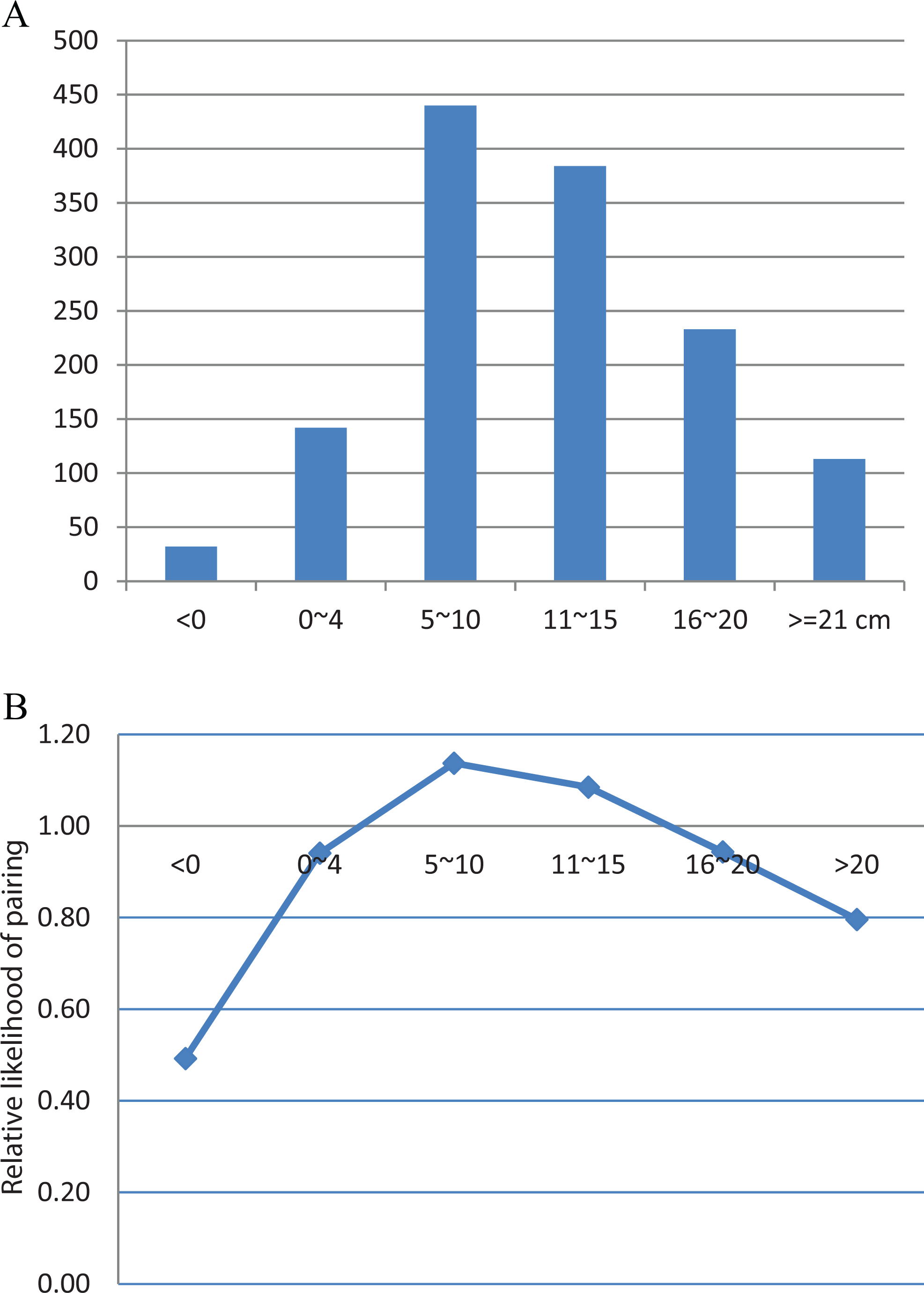
(A) Frequency distribution of parental height differences. (B) Relative likelihood of pairing. The relative likelihood of pairing which is the actual frequency observed in the population divided by the simulated frequency resulting from random pairing. The sample size for Figure 2 is 1,344.

Whether assortative mating with respect to height varies with age cohort, educational level, and family income was explored further in Table 2. The correlation coefficients between the height of male and female spouses were significant in all groups, indicating that the assorative mating with respect to height prevailed in all groups. The correlation coefficients for the old cohort were greater than the young cohort. Likewise, the association between the heights of male and female spouses was greater for high family income group than low family income group. As on average, the old were richer than the young, it is possible that the relationship between family income and spouse’s height is a reflection of the relationship between age and family income.

Table 2.

Correlation Coefficients Between Husband’s and Wife’s Height by Age, Education, Family Income, and Sex.

Sex	Young	Old	Low Education	High Education	Low Income	High Income
Men
r	.170	.288	.196	.273	.181	.267
p Value	<.001	<.001	<.001	<.001	<.001	<.001
Number of observations	728	616	938	406	744	600
Women
r	.204	.253	.213	.241	.181	.267
p Value	<.001	<.001	<.001	<.001	<.001	<.001
Number of observations	694	650	1,089	255	744	600

Note. Table 2 divides age, educational attainment, and family income into two groups. The number of observations is 1,344. Husbands younger or equal to 40 (median) years old were classified into the young group, whereas others into the old group. The median age for wives was 37, and the same classification rule was applied. Educational attaintment less than or equal to high school was defined as low education, whereas higher than high school was high education. Family income less than or equal to the median family income, NT$55,000, was low family income, and high family income if greater than the median family income.

Simulated Distribution and Actual Distribution

Among the 1,344 couples, there were only 32 couples where the wife was taller than the husband, comprising only 2.38% of the sample (see Table 3), compared to 4.09% in Stulp, Buunk, Pollet, et al. (2013). Of course, as in this sample, husbands on average were taller than their wives by more than 11 cm, it was expected by chance that husbands were taller than wives in most cases. However, if assortative mating in the marriage market indeed conforms to the male-taller norm, then this 2.38% would be significantly less than the breakage proportion of the male-taller norm resulting from a random sorting.

Table 3.

Random Height Sorting Based on 200 Simulations.

Wife taller than husband	Number of Wife’s Height > Husband’s Height	Percentage (%)	Z	p
Maximal cases	84	6.25	–5.86	<.001
Average cases	65	4.84	–4.20	<.001
Minimal cases	46	3.42	–2.10	.018
Actual cases	32	2.38

Note. “Maximal cases” indicates the maximal number of times that wife is taller than her husband in one of these 200 random simulations. “Minimum cases” has a similar but reversal meaning. “Average cases” is the average number of cases that a wife is taller than her husband in these 200 simulations. “Actual cases” is the actual number of cases that a wife is taller than her husband in the sample. The percentage is the number in the first column divided by the sample size 1,344. The last column is the Z-value testing if the percentage is significantly different with the actual percentage, 2.38.

Table 3 records the maximal and minimal number of cases in which a wife was taller than her husband in the 200 random simulations. The maximal number and the minimal number of cases violating the male-taller norm were 84 and 46, respectively. Both numbers were much higher than the actual number of violation cases, 32. The frequency of violation cases, that is, a wife taller than her husband, in each simulation was never less than 32. The second column of Table 3 shows the percentage of cases violating the male-taller norm. The percentage of the cases violating the male-taller norm for the maximal number of cases was 6.25%, while for the minimal number of cases, it was 3.42%; both percentages were greater than the actual violation percentage, 2.38%. The third column presents Z tests for the percentages of the cases violating the male-taller norm in the random sorting with respect to the actual violation percentage. All three Z values significantly rejected the null hypothesis that violation percentages for the cases in the random sorting were equal to or less than the actual violation percentage.

The difference between the actual violation percentage and the violation percentage generated from 200 random simulations was small. From another angle, the difference in the number of violation cases between the actual situation and the simulations was substantial. The actual number of violation cases was 32, but the average amount of violation cases in the 200 simulations was 65. This means that about half the number of male-taller violation cases were avoided. This provides evidence of the male-taller norm. Furthermore, because most males were taller than females, the percentages of violation cases in the simulations were small. By its very nature, the difference of the violation percentages between the actual situation and the random simulation was also small. But this small percentage difference cannot be used to deny the male-taller norm.

The first row of Table 4 presents the actual counts regarding height difference between husband and wife. The second row shows the median counts of 200 random simulations by height difference. The values in the third row are the p values for each height difference category. For example, in the 200 simulations, none of the simulated counts in the “less than 0” category were less than or equal to the actual counts, 32, so the p value obtained was less than 1/200 = .005. This p value corresponds to the directional hypothesis that the simulated counts are either over- or underrepresented compared to the actual counts (Stulp, Buunk, Pollet, et al., 2013). The p values for the categories of less than 0, 0–4, 16–20, and greater than 21 were left tailed, while the p values for 5–10 and 11–15 were right tailed. The actual counts in the 5–10 and 11–15 cm categories were significantly higher than what would be expected by chance, while the actual counts in the categories less than 5 cm and greater than 20 cm were significantly lower than what would be expected by chance. Due to the missing values of explanatory variables, 723 couples are deleted. Using the same simulation approach, the same results are obtained from the 2,067 couples. That is, the actual counts of height difference between 5 and 15 cm were higher than what would be expected by chance. The deletion of observations does not change the conclusion.

Table 4.

Actual and Simulated Counts of Height Differences.

Height Difference (cm)	Less Than 0	0–4	5–10	11–15	16–20	Greater Than 21
Actual counts	32	142	440	384	233	113
Median counts	65	151	387	354	247	142
p Value	<.005	.160	<.005	.005	.145	<.005
Relative likelihood of pairing	0.492	0.940	1.137	1.085	0.943	0.796

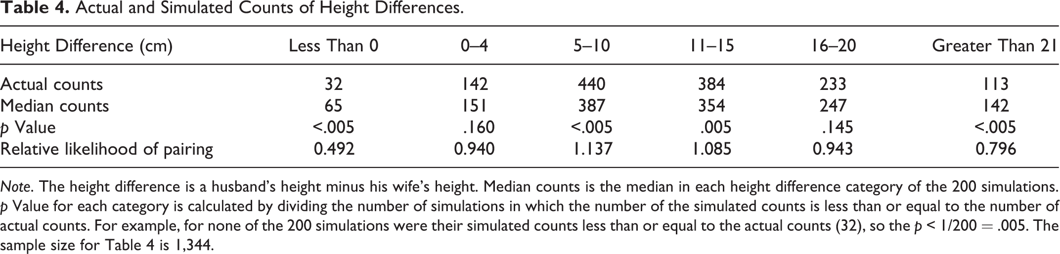
Note. The height difference is a husband’s height minus his wife’s height. Median counts is the median in each height difference category of the 200 simulations. p Value for each category is calculated by dividing the number of simulations in which the number of the simulated counts is less than or equal to the number of actual counts. For example, for none of the 200 simulations were their simulated counts less than or equal to the actual counts (32), so the p < 1/200 = .005. The sample size for Table 4 is 1,344.

Ordered Probit Models

The advantage of regression is that it can control for other factors and specifically focus on the pure relationship between the heights of husbands and wives. In Table 5, the dependent variables of the left panel and right panel are husband’s height and wife’s height, respectively. The middle group of spouse’s height was the comparison reference and is not shown in Table 5. The left panel and the right panel of Table 5, respectively, show the husband and wife results of the ordered probit models. Height between 155 and 160 cm was the wife height reference group, while height between 166 and 170 cm was the husband height reference group. In other words, the groups of average heights for males and females were used as the respective reference groups. Neither reference group was shown in the table. The explanatory variables included four categories of spouse height, respondents’ and spouse’s educational years and age, and logarithm family income. Family income was taken as the logarithm because the ordered probit models cannot converge if the family income did not take a logarithm. Spouse’s age was not incorporated into the explanatory variables due to a multicollinearity concern. In this sample, the correlation coefficient between a husband’s age and his wife’s age was .72. When spouse’s age was included in the model, the coefficient of spouse’s age in either husband model or in wife model showed a reverse sign as expected. We expected that the young generation would be taller than the old generation, but the coefficients of spouse’s age were significantly positive, indicating that old spouses were coupled with tall respondents. Given the high correlation between spouse’s ages, this is likely to be a consequence of multicollinearity. Therefore, the spouse’s age was excluded. In fact, Dormann et al. (2013) indicated that multicollinearity begins to severely distort model estimation when |r| > .7. Tabachnick and Fidell (2014) also suggested deleting the highly correlated variable when |r| > .7.

Table 5.

Results of Ordered Probit Models by Sex.

Husband	Coefficient	t	p	Wife	Coefficient	t	p
Constant	–0.408	–0.64	.519	Constant	–0.321	–0.51	.610
Wife height (cm)				Husband height (cm)
≤150	–0.401	–3.88	<.001	≤160	–0.575	–4.42	<.001
151–155	–0.127	–1.69	.091	161–165	–0.178	–2.18	.030
161–165	0.171	2.16	.030	171–175	0.085	1.14	.252
>165	0.600	4.37	<.001	>175	0.397	4.14	<.001
Husband education	0.038	2.82	.005	Husband education	0.040	2.91	.004
Husband age	–0.040	–6.51	<.001	Wife age	–0.007	–0.50	.619
Wife education	0.028	1.93	.054	Wife education	–0.011	–1.81	.071
Log (family income)	0.273	4.49	<.001	Log(family income)	0.158	2.60	.009
μ₁	0.968	26.06	<.001	μ₁	0.870	25.61	<.001
μ₂	2.068	57.52	<.001	μ₂	2.049	53.73	<.001
μ₃	2.962	62.95	<.001	μ₃	2.991	52.99	<.001

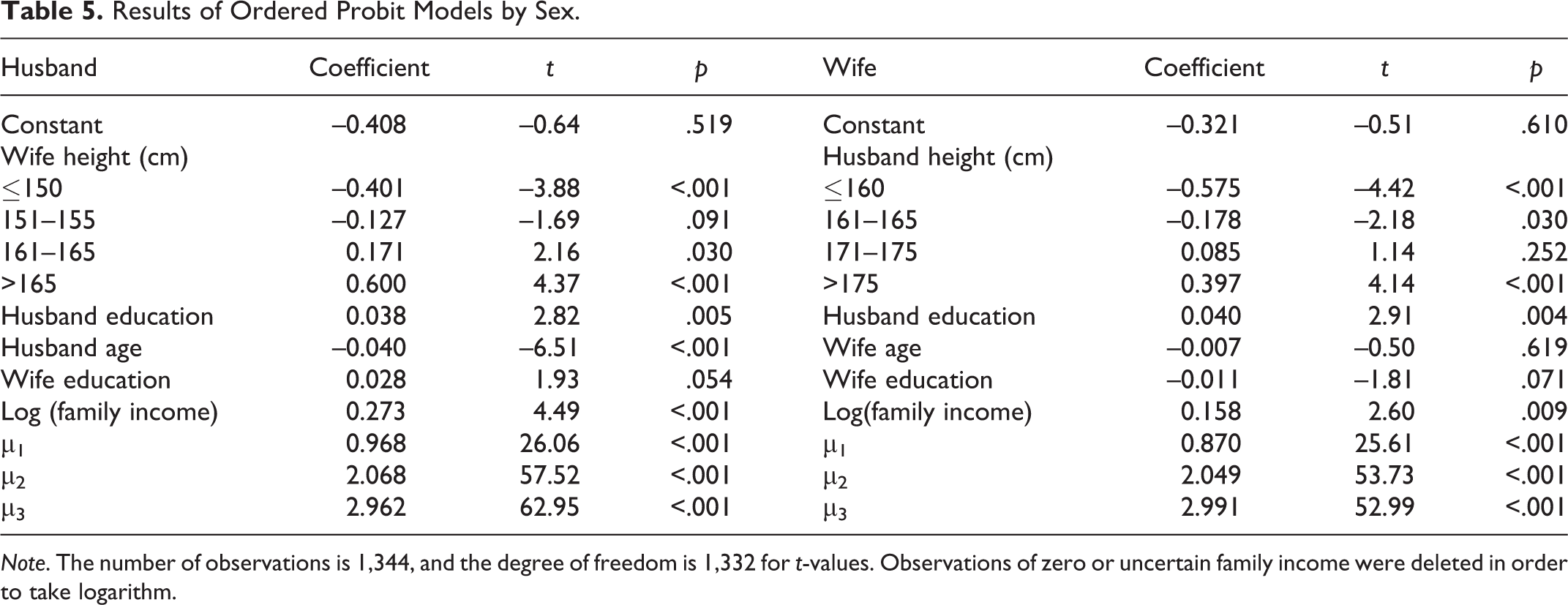
Note. The number of observations is 1,344, and the degree of freedom is 1,332 for t-values. Observations of zero or uncertain family income were deleted in order to take logarithm.

In the left panel, the coefficients of wife’s height categories shorter than and taller than the average height group were negatively and positively significant at least at the 10% level, respectively. Husband’s education and age were respectively positively and negatively significant at the 1% level. Husbands with higher educational attainment and younger age were taller. Highly educated wives were coupled with tall men. Rich families had tall husbands.

The right panel of Table 5 shows the results for wives. The coefficients of husband height categories shorter than 166 were significant at the 5% level. The coefficient of the tallest husband category was significant, while that of 171–175 group was not significant. Although for women it seems to indicate that husband’s height were indistinguishable between the height groups of 171–175 and 166–170, the next table (marginal probability table) shows that men of 171–175 had a significantly different chance to be married to women of a different height category. The absolute values of the coefficients of age and family income and their t-values in the right panel were smaller than husband’s corresponding values in the left panel.

Notably, ordered probit models are not linear. Unlike coefficients of ordinary least squares (OLS) models, coefficients of ordered probit models are not marginal effects of their corresponding variables. The marginal effects are in terms of probability and vary with the quantity of the independent variables in question. Computer software provides a marginal probability effect of an independent variable at its average and at the other variables’ averages. The marginal probability effect of a dummy variable, such as spouse height groups, is the probability change from the reference group to a group in question.

The top and bottom panels of Table 6 exhibit the marginal probability effects of the ordered probit models as husband’s height and wife’s height are the dependent variables, respectively. Each independent variable was associated with five marginal probability effects. For example, in the top panel, the five marginal probability effects of husband’s education were −.004, −.008, −.003, .007, and .007. Each of these five marginal probabilities corresponded to each husband height category in the top row. The probabailty −.004 meant that an increment of 1 year of education decreased the probability by .004 of falling in the category of less than or equal to 160 cm. By the same token, the increment of 1 year of education decreased the probability by .008 and .003, respectively, falling into the 161–165 and 166–170 cm categories, and increased the probability by .007 and .007, respectively, falling into the 171–175 and >175 cm categories. These five marginal probabilities were calculated using Equation 4, and their sum was zero. The marginal probability of a husband’s educational attainment was negative and became positive as a husband’s height increased. This property reflects the positive coefficient of husband’s educational attainment in Table 5.

Table 6.

Marginal Probability of Independent Variables by Each Height Category.

Husband Height
Wife height	≤160		161—165		166–170		171–175		>175
Wife height	Coefficient	p	Coefficient	p	Coefficient	p	Coefficient	p	Coefficient	p
≤150	0.050	<.001	0.086	<.001	0.003	.984	–0.080	.484	–0.058	<.001
t	116.86		19.73		0.02		–0.70		–4.43
151–155	0.013	<.001	0.027	<.001	0.007	.924	–0.025	.828	–0.022	.014
t	5.62		4.52		0.10		–0.22		–2.47
161–165	–0.015	<.001	–0.035	<.001	–0.015	.107	0.032	.813	0.033	<.001
t	–3.57		–4.26		–1.61		0.24		5.03
>165	–0.036	<.001	–0.109	<.001	–0.090	.000	0.089	.654	0.146	<.001
t	–6.50		–9.36		–12.32		0.45		10.71
Husband edu	–0.004	.005	–0.008	.005	–0.003	.829	0.007	.013	0.007	.007
t	–2.79		–2.82		–0.22		2.48		2.68
Husband age	0.004	<.001	0.008	<.001	0.003	.829	–0.008	<.001	–0.007	<.001
t	6.14		6.50		0.22		–4.33		–4.64
Wife education	–0.003	.056	–0.006	.054	–0.002	.829	0.005	.062	0.005	.067
t	–1.92		–1.93		–0.22		1.86		1.83
Family income	–0.026	<.001	–0.058	<.001	–0.018	.837	0.053	.012	0.049	<.001
t	–4.36		–4.48		–0.21		2.50		3.78
Wife Height
Husband height	≤150		151–155		156–160		161–165		>165
≤160	0.125	<.001	0.095	<.001	–0.073	.631	–0.107	.536	–0.040	<.001
t	224.98		19.82		–0.48		–0.62		–3.46
161–165	0.030	<.001	0.034	<.001	–0.011	.745	–0.037	.793	–0.017	.008
t	8.25		6.15		–0.33		–0.26		–2.66
171–175	–0.013	.028	–0.017	.01550	0.003	.960	0.018	.889	0.009	.014
t	–2.20		–2.42		0.05		0.14		2.47
>175	–0.051	<.001	–0.077	<.001	–0.008	.953	0.083	.529	0.053	<.001
t	–6.35		–8.60		–0.06		0.63		5.50
Husband edu	–0.006	.004	–0.008	.00360	0.002	.917	0.008	.227	0.004	.016
t	–2.89		–2.91		0.10		1.21		2.42
Wife age	0.001	.619	0.001	.61850	0.000	.917	–0.002	.657	–0.001	.622
t	0.50		0.50		–0.11		–0.44		–0.49
Wife education	0.002	.072	0.002	.071	0.000	.918	–0.002	.234	–0.001	.089
t	1.80		1.81		–0.10		–1.19		–1.70
Family income	–0.025	.010	–0.031	.009	0.006	.914	0.033	.392	0.017	.019
t	–2.58		–2.60		0.11		0.86		2.34

Note. The number of observations and the degree of freedom are the same with Table 5.

In the top panel of Table 6, wife’s height between 156 and 160 cm was the reference group which is not shown in the table. Any marginal probability of the wife’s height category was the difference between that category and the reference category. For example, the first value in the first column (.050) meant that a wife measuring less than or equal to 150 cm was more likely than a wife in the reference group to be married to a husband with a height of less than or equal to 160 cm by a probability of .050. This marginal probability was significant at the 1% level. Taking the category of wife height between 161–165 cm as an example, compared to the reference group, the marginal probability of women in this height category being coupled with a man whose height was less than or equal to 160, 161–165, 166–170, 171–175, and >175 cm were −.015, −.035, −.015, .032, and .033, respectively. Compared to the height reference group, women in the taller groups were more unlikely to be married to a man shorter than 171 cm and more likely to be married to a man taller than 175 cm. With wives who were taller than the reference group, the absolute value of the negative marginal probability increased with women’s height, suggesting that taller women were more unlikely to be married to short men. Likewise, the positive marginal probability of the taller women also increased with women’s height, indicating that taller women were more likely to be married to tall men. When wives were shorter than the reference group, the positive marginal probability and the absolute value of the negative marginal probability decreased as wife’s height increased. These figures indicated that short women were more likely to be married to short men and less likely to be married to tall men, respectively.

Positive values in Table 6 indicated that the height match in question had a higher probability to occur than the corresponding match in the reference group. Wives shorter than 156 cm were more likely to be married to husbands shorter than 166 cm. The height difference between a husband and wife was approximately within a range of 5 (160 − 155) to 15 (165 − 150) cm. Wives taller than 160 cm were more likely to be married to husbands taller than 175 cm. In this case, the height difference between a husband and his wife was approximately within a range of 10 (175 − 165) to 15 (175 − 160) cm.

In the bottom panel, the coefficients of husband’s height showed a similar pattern to the top panel. Notably, compared to the reference group (husband’s height between 166 and 170 cm), husbands shorter than 166 cm were more likely to be married to wives shorter than 156 cm. The height difference was approximately 5 (160 − 155) to 15 (165 − 150) cm. Husbands taller than 170 cm were more likely to be married to a wife taller than 165 cm. The height difference was also roughly within the range of 5 (170 − 165) to 10 (175 − 165) cm.

Discussion

The height data from the ESCNHS were self-reported. Although measured height is more precise than self-reported height, several studies have reported that these two measurements are highly correlated. For example, Spencer, Appleby, Davey, and Key (2002) and Wada et al. (2005) reported that correlation coefficients between measured and self-reported height were greater than .9 for British persons, .979 for Japanese men, and .988 for Japanese women, respectively. People tend to overreport their height and to underreport their weight. Using self-reported stature to calculate body mass index might therefore underestimate the problem of obesity (Spencer, Appleby, Davey, & Key, 2002). However, the bias of using self-reported height to investigate height difference between a husband and his wife is limited as both sexes tend to overreport their height and the overestimates will be canceled out. There is no agreement about which sex overreports their height more than the other sex. Some studies found that men overreported their height more than women (Krul, Daanen, & Choi, 2011), some indicated that men and women overreported their height by the same magnitude (Wada et al., 2005), and some even found that women overreported more than men (Lucca & Moura, 2010).

In each society, there seems to exist an ideal height difference between a male and his female spouse. The ideal range of height difference consists of an upper and lower bound. This ideal range of height difference in the United Kingdom is probably 0–25 cm (Stulp, Buunk, Pollet, et al., 2013), and it is 5–15 cm in Taiwan. The stereotype gender role implies that a husband has to be significantly taller than his wife. Hence, the sex-role impression cannot be created when the height difference between a couple is less than the lower bound of the ideal range. If shortness reflects liabilities of personal traits (Agerström, 2014; Jackson & Ervin, 1992; Judge & Cable, 2004), then women dislike looking too short for their partners. Men also dislike their partners to look too short relative to themselves. This societal expectation constructs the upper bound of the ideal range of the height difference between a couple. Women prefer a mate taller than themselves. Evolutionary psychology and resource access can explain this male-taller norm phenomena. However, these two hypotheses cannot explain why women do not prefer a mate much taller than themselves. If tall men are a symbol of dominance, competitiveness, and resource access, then all women, regardless of their own height, will desire the same group of tall men. But this contradicts what we observed. The recent finding of the male-not-too-tall norm implies more hypotheses are needed to explain why women prefer a mate taller but not much taller than themselves.

The lower bound is probably determined by the societal characteristics, in particular the degree of sex equality. The degree of sex stereotype is low in sex equal societies, and consequently, these societies possess a small lower bound of the ideal range of the height difference. The Global Gender Gap Index (GGGI) was constructed by the World Economic Forum to measure sex equality among countries. A large GGGI indicates a highly sex equal society. The lower bound of the height difference observed in the United Kingdom is 0, while in Taiwan is 5. Correspondingly, the GGGI for the United Kingdom in 2014 was .7383, greater than the GGGI for Taiwan in the same year which was .7214.¹

The upper bound of the ideal range is likely to vary with societal expectation and the stature property of a population. From the perspective of the stature property, Euopeans are taller than Asians. It seems that tall populations have a greater upper bound than short populations. As tall populations have a greater height variance than short populations (Schmitt & Harrison, 1988), a great upper bound of the ideal height difference in tall populations is able to contain a sufficiently large pool of mates. This stature property of a population might be the biological basis of the formation of societal expectation. In other words, a male taller than his female spouse by more than the upper bound would be seen as a weird couple which actually implies that a sufficiently large pool of mates has been reached with a smaller height difference in this population. This might explain why the observed upper bound of the height difference in Taiwan was smaller than in the United Kingdom. Cohen (2013) published a nonacademic article in the Atlantic. He used 4,600 couples from the data set of the Panel Study of Income Dynamics of the United States in 2009 to run 10 random simulations for height match. From the figure he drew, the actual height difference was roughly within a range between −0.5 and 22 cm (−0.2 and 8.5 in.) which occurred more often than expected by chance. The GGGI for the United States in 2014 was .7463, greater than the United Kingdom. The range of height difference occurring more than expected in the United States was in line with the aforementioned arguments. However, the lack of studies on this issue does not allow us to make a persuasive conclusion. Further studies are encouraged to explore this issue in different populations.

This study used Taiwanese data to examine the prevalence of the male-taller and the male-not-too-tall norms in Taiwan. Consistent with previous studies using Western populations (Pawlowski, 2003; Salska et al., 2008; Swami et al., 2008), the relative height for Taiwanese couples was large for tall men and short women and small for short men and tall women. This provides evidence for the male-taller norm because tall men and short women have a greater buffer than short men and tall women to conform to the male-taller norm. As expected, the shorter the husband or the taller the wife, the more likely the violation of the male-taller norm. The uneven distribution of the number of cases violating the male-taller norm is also evidence for the male-taller norm because short men and tall women find it more difficult to avoid the violation of the male-taller norm. Women want taller men more than men want shorter women (Stulp, Buunk, Kurzban, & Verhulst, 2013; Stulp, Buunk, & Pollet, 2013). From another perspective, the high violation proportion of the male-taller norm for tall women indicates that the male-taller norm is not essential. After all, stature is only one of multiple dimensions considered in a marriage. In addition, the taller the husbands, the more family income and years of education they had. These results were in line with the findings in the literature (Böckerman & Vainiomäki, 2013; Case & Paxson, 2008; Cinnirella et al., 2011; Meyer & Selmer, 1999; Kortt & Leigh, 2010; Lundborg et al., 2014; Magnusson et al., 2006; Persico et al., 2004; Silventionen et al., 1999; Szklarska et al., 2007).

An OLS model can verify the overall relationship between husband’s height and wife’s height by controlling for other factors. However, this continuous variable model cannot examine which height group of women is more likely to be coupled with which height group of men. This is why the continuous variable of height was categorized, and an ordered probit model was applied. The subjective categorization on height implies that the application of the ordered probit model is not a perfect methodology, but it gives alternative results and conclusions that an OLS model would be unable to give. With the control of other factors, an OLS model can verify the male-taller norm, but it cannot verify the male-not-too-tall norm. An ordered probit model is able to verify the male-taller norm as well as the male-not-too-tall norm at the same time. The results of the ordered probit models demonstrated that tall men were more likely to be coupled with tall women, whereas short men were more likely to be coupled with short women. These results verified the prevalence of the male-taller norm in Taiwan. The results of the ordered probit models further confirmed the prevalence of the male-not-too-tall norm in Taiwan. The frequency of the height difference between a husband and his wife to be within the range of 5–15 cm was significantly higher than other ranges. This range was consistent with the result of the random simulations.

Using Indonesian data, Sohn (2015) found that 93.4% of actual couples were in line with the male-taller norm, statistically more than 88.8% of random couples. Despite the significant difference between random mating and actual mating, Sohn (2015) argued that the small difference only made statistical sense and concluded a lack of evidence for the male-taller norm in Indonesia. The difference of violation ratios between the actual mating and the random mating in Taiwan was only about 2.5% on average, but this study showed that this small difference still differed from chance. The average number of cases violating the male-taller norm in the random mating was more than 2 times the size of the actual mating.

Preferred characteristics and actual characteristics of mates usually differ (Courtiol, Picq, Godelle, Raymond, & Ferdy, 2010). This difference occurs for at least two reasons. First, preferred characteristics are usually compromised in actual matches (Stulp, Buunk, Kurzban, et al., 2013). Second, a positive association between the heights of a man and his female spouse from the actual couple data might reflect the assortative mating with respect to factors other than height. For example, we have seen that educational attainment was positively correlated with height. The assortative mating with respect to education also supports the positive association between the heights of a male and of his female spouse. This was of course not the case for the present study because the ordered probit models controlled for educational attainment. However, it is still possible that the positive association of the heights between a couple is due to some other unobserved factors.

Footnotes

Declaration of Conflicting Interests

The author(s) declared no potential conflicts of interest with respect to the research, authorship, and/or publication of this article.

Funding

The author(s) received no financial support for the research, authorship, and/or publication of this article.

Note

References

Agerström

(2014). Why does height matter in hiring? Journal of Behavioral and Experimental Economics, 52, 35–38.

Becker

N. S.

Touraille

Froment

Heyer

Courtiol

(2012). Short stature in African pygmies is not explained by sexual selection. Evolution and Human Behavior, 33, 615–622.

Blaker

N. M.

Rompa

Dessing

I. H.

Vriend

A. F.

Herschberg

Van Vugt

(2013). The height leadership advantage in men and women: Testing evolutionary psychology predictions about the perceptions of tall leaders. Group Processes & Intergroup Relations, 16, 17–27.

Böckerman

Vainiomäki

(2013). Stature and life-time labor market outcomes: Accounting for unobserved differences. Labour Economics, 24, 86–96.

Buss

D. M.

Barnes

(1986). Preferences in human mate selection. Journal of Personality and Social Psychology, 50, 559.

Campos

G. E.

Luecke

T. J.

Wendeln

H. K.

Toma

Hagerman

F. C.

Murray

T. F.

… Staron

R. S.

(2002). Muscular adaptations in response to three different resistance-training regimens: Specificity of repetition maximum training zones. European Journal of Applied Physiology, 88, 50–60.

Case

Paxson

(2008). Stature and status: Height, ability, and labor market outcomes. Journal of Political Economy, 116, 499–532.

Cinnirella

Piopiunik

Winter

(2011). Why does height matter for educational attainment? Evidence from German children. Economics and Human Biology, 9, 407–418.

Cohen

(2013, 1 28). Why it’s so rare for a wife to be taller than her husband. The Atlatic. http://www.theatlantic.com/sexes/archive/2013/01/why-its-so-rare-for-a-wife-to-be-taller-than-her-husband/272585/.

10.

Courtiol

Picq

Godelle

Raymond

Ferdy

J. B.

(2010). From preferred to actual mate characteristics: The case of human body shape. PLoS ONE, 5, e13010.

11.

Courtiol

Raymond

Godelle

Ferdy

J. B.

(2010). Mate choice and human stature: Homogamy as a unified framework for understanding mating preferences. Evolution, 64, 2189–2203.

12.

Dormann

C. F.

Elith

Bacher

Buchmann

Carl

Carré

… Münkemüller

(2013). Collinearity: A review of methods to deal with it and a simulation study evaluating their performance. Ecography, 36, 27–46.

13.

Fink

Neave

Brewer

Pawlowski

(2007). Variable preferences for sexual dimorphism in stature (SDS): Further evidence for an adjustment in relation to own height. Personality and Individual Differences, 43, 2249–2257.

14.

Gillis

J. S.

Avis

W. E.

(1980). The male-taller norm in mate selection. Personality and Social Psychology Bulletin, 6, 396–401.

15.

Heineck

(2005). Up in the skies? The relationship between body height and earnings in Germany. Labour, 19, 469–489.

16.

Higgins

L. T.

Zheng

Liu

Sun

C. H.

(2002). Attitudes to marriage and sexual behaviors: A survey of gender and culture differences in China and United Kingdom. Sex Roles, 46, 75–89.

17.

Jackson

L. A.

Ervin

K. S.

(1992). Height stereotypes of women and men: The liabilities of shortness for both sexes. The Journal of Social Psychology, 132, 433–445.

18.

Judge

T. A.

Cable

D. M.

(2004). The effect of physical height on workplace success and income: Preliminary test of a theoretical model. Journal of Applied Psychology, 89, 428–441.

19.

Koestner

Wheeler

(1988). Self-presentation in personal advertisements: The influence of implicit notions of attraction and role expectations. Journal of Social and Personal Relationships, 5, 149–160.

20.

Komlos

Kriwy

(2002). Social status and adult heights in the two Germanies. Annals of Human Biology, 29, 641–648.

21.

Kortt

Leigh

(2010). Does size matter in Australia? Economic Record, 86, 71–83.

22.

Krul

A. J.

Daanen

H. A.

Choi

(2011). Self-reported and measured weight, height and body mass index (BMI) in Italy, the Netherlands and North America. European Journal of Public Health, 21, 414–419.

23.

Krzyżanowska

Mascie-Taylor

C. N.

(2011). Intra-and intergenerational social mobility in relation to height, weight and body mass index in a British national cohort. Journal of Biosocial Science, 43, 611–618.

24.

Krzyżanowska

Mascie Taylor

C. G.

Thalabard

J. C.

(2015). Is human mating for height associated with fertility? Results from a British national cohort study. American Journal of Human Biology, 27, 553–563.

25.

Lucca

Moura

E. C.

(2010). Validity and reliability of self-reported weight, height and body mass index from telephone interviews. Cadernos de Saúde Pública, 26, 110–122.

26.

Lundborg

Nystedt

Rooth

D. O.

(2014). The height premium in earnings: The role of cognitive and non-cognitive skills. Journal of Human Resources, 49, 41–166.

27.

Magnusson

P. K.

Rasmussen

Gyllensten

U. B.

(2006). Height at age 18 years is a strong predictor of attained education later in life: Cohort study of over 950 000 Swedish men. International Journal of Epidemiology, 35, 658–663.

28.

Meyer

H. E.

Selmer

(1999). Income, educational level and body height. Annals of Human Biology, 26, 219–227.

29.

Murray

G. R.

Schmitz

J. D.

(2011). Caveman politics: Evolutionary leadership preferences and physical stature. Social Science Quarterly, 92, 1215–1235.

30.

Pawlowski

(2003). Variable preferences for sexual dimorphism in height as a strategy for increasing the pool of potential partners in humans. Proceedings of the Royal Society of London B: Biological Sciences, 270, 709–712.

31.

Pawlowski

Koziel

(2002). The impact of traits offered in personal advertisements on response rates. Evolution and Human Behavior, 23, 139–149.

32.

Persico

Postlewaite

Silverman

(2004). The effect of adolescent experience on labor market outcomes: The case of height. Journal of Political Economy, 112, 1019–1053.

33.

Pierce

C. A.

(1996). Body height and romantic attraction: A meta-analytic test of the male-taller norm. Social Behavior and Personality: An International Journal, 24, 143–150.

34.

Salska

Frederick

D. A.

Pawlowski

Reilly

A. H.

Laird

K. T.

Rudd

N. A.

(2008). Conditional mate preferences: Factors influencing preferences for height. Personality and Individual Differences, 44, 203–215.

35.

Schmitt

L. H.

Harrison

G. A.

(1988). Patterns in the within-population variability of stature and weight. Annals of Human Biology, 15, 353–364.

36.

Sear

(2010). Height and reproductive success: Is bigger always better? In Frey

U. J.

Stormer

Willfuhr

K. P.

(Eds.), Homo novus: A human without illusions. The Frontiers Collection (pp. 127–143). Heidelberg, Germany: Springer.

37.

Sear

Marlowe

F. W.

(2009). How universal are human mate choices? Size does not matter when Hadza foragers are choosing a mate. Biology Letters, 5, 606–609.

38.

Shepperd

J. A.

Strathman

A. J.

(1989). Attractiveness and height the role of stature in dating preference, frequency of dating, and perceptions of attractiveness. Personality and Social Psychology Bulletin, 15, 617–627.

39.

Silventoinen

Lahelma

Rahkonen

(1999). Social background, adult body-height and health. International Journal of Epidemiology, 28, 911–918.

40.

Silventoinen

Lahelma

Lundberg

Rahkonen

(2001). Body height, birth cohort and social background in Finland and Sweden. The European Journal of Public Health, 11, 124–129.

41.

Sohn

(2015). The male-taller norm: Lack of evidence from a developing country. HOMO-Journal of Comparative Human Biology, 66, 369–378.

42.

Sorokowski

Butovskaya

M. L.

(2012). Height preferences in humans may not be universal: Evidence from the Datoga people of Tanzania. Body Image, 9, 510–516.

43.

Sorokowski

Sorokowska

(2012). Judgments of sexual attractiveness: A study of the Yali tribe in Papua. Archives of Sexual Behavior, 41, 1209–1218.

44.

Sorokowski

Sorokowska

Butovskaya

Stulp

Huanca

Fink

(2015). Body height preferences and actual dimorphism in stature between partners in two non-Western societies (Hadza and Tsimané). Evolutionary Psychology, 13, 455–469.

45.

Spencer

E. A.

Appleby

P. N.

Davey

G. K.

Key

T. J.

(2002). Validity of self-reported height and weight in 4808 EPIC–Oxford participants. Public Health Nutrition, 5, 561–565.

46.

Stulp

Buunk

A. P.

Kurzban

Verhulst

(2013). The height of choosiness: Mutual mate choice for stature results in suboptimal pair formation for both sexes. Animal Behaviour, 86, 37–46.

47.

Stulp

Buunk

A. P.

Pollet

T. V.

(2013). Women want taller men more than men want shorter women. Personality and Individual Differences, 54, 877–883.

48.

Stulp

Buunk

A. P.

Pollet

T. V.

Nettle

Verhulst

(2013). Are human mating preferences with respect to height reflected in actual pairings. PLoS ONE, 8, e54186.

49.

Stulp

Buunk

A. P.

Verhulst

Pollet

T. V.

(2013). Tall claims? Sense and nonsense about the importance of height of US presidents. The Leadership Quarterly, 24, 159–171.

50.

Stulp

Mills

Pollet

T. V.

Barrett

(2014). Non-linear associations between stature and mate choice characteristics for American men and their spouses. American Journal of Human Biology, 26, 530–537.

51.

Swami

Furnham

Balakumar

Williams

Canaway

Stanistreet

(2008). Factors influencing preferences for height: A replication and extension. Personality and Individual Differences, 45, 395–400.

52.

Szklarska

Koziel

Bielicki

Malina

R. M.

(2007). Influence of height on attained level of education in males at 19 years of age. Journal of Biosocial Science, 39, 575–582.

53.

Tabachnick

B. G.

Fidell

L. S.

(2014). Using multivariate statistics. London, England: Pearson.

54.

Wada

Tamakoshi

Tsunekawa

Otsuka

Zhang

Murata

… Toyoshima

(2005). Validity of self-reported height and weight in a Japanese workplace population. International Journal of Obesity, 29, 1093–1099.

55.

Yancey

Emerson

M. O.

(2016). Does height matter? An examination of height preferences in romantic coupling. Journal of Family Issues, 37, 53–73.

Male-Taller and Male-Not-Too-Tall Norms in Taiwan

Abstract

Keywords

Material and Method

Sample

Method

Random Simulation

Ordered Probit Model

Results

Assortative Mating

Simulated Distribution and Actual Distribution

Ordered Probit Models

Discussion

Footnotes

Declaration of Conflicting Interests

Funding

Note

References