CMGV: Algorithms and a unified framework for complexity management in graph visualization

Abstract

Illustrating data visually through graphs enables the examination of valuable insights and the identification of crucial patterns that are beneficial for the user. However, as the volume of data grows, it becomes increasingly challenging to organize corresponding graphs and zero in on specific objects and/or relations of interest. Various techniques have been developed to tackle the complexity of large graphs, yet these methods operate independently, potentially resulting in inconsistencies and incorrect behaviors, as well as inefficient use of computing resources when mixed together and applied in a certain order. Furthermore, administering these methods can lead to significant changes in the layout of the graph, potentially disorienting the user and disrupting their mental map. This study aims to design a framework and associated algorithms for efficiently and effectively managing complexity during visual analysis of large relational data represented as graphs, by seamlessly integrating various complexity management techniques and making adjustments to the graph layout after each operation to preserve the user’s mental map. A rendering-independent implementation of this framework and associated algorithms, as well as its integration with a popular graph rendering library named Cytoscape.js, can be accessed freely on GitHub.

Introduction

The rapid accumulation of data in today’s world requires efficient analysis to make informed decisions in all kinds of industries. Visualization aids in this analysis by highlighting patterns, relationships, and trends for a better understanding.

Graphs or networks are a popular way to represent relational data visually. A clear layout of objects and links is essential for understanding the information presented in a graph. Poor layouts can lead to confusion for the viewer, and users may spend a significant amount of time adjusting the layout manually. ¹ As a result, a reliable automatic layout feature is crucial for software that performs graph visualization-based analysis. ² The idea of using compound graphs, ³ where nodes can hold entire other graphs within them, allowing for easy nesting, is a popular way to depict intricate connections and different levels of abstraction in data.

Effective analysis of large networks, such as those in systems biology, requires the ability to interact with and navigate the network quickly.^4,5 However, traditional methods for performing operations on these networks, such as automatic layout or calculating graph-theoretic properties, do not scale well. Additionally, even if the entire network can be rendered on a computer display, the resulting visualization may be overwhelming and difficult to understand. To overcome these challenges, complexity management techniques are used to reduce the complexity of the network.^5–8 Such techniques include filtering nodes or edges, collapsing compound nodes, and temporarily hiding parts of the topology.

Various methods and software libraries have been developed to manage the complexity of large graphs, but they happen to work independently, which can cause inconsistencies and incorrect results as well as inefficient use of computing resources when applied in certain mixed orders (see Figure 9 for examples). Additionally, using these methods can lead to significant changes in the layout of the graph, which can cause confusion and disrupt the user’s mental map of the data.

To fill this void, this paper introduces a novel framework named CMGV (Complexity Management in Graph Visualization) for efficiently and effectively managing complexity during the visual analysis of large relational data represented as graphs. Our design seamlessly integrates various complexity management techniques and continuously adapts the graph layout to preserve the user’s understanding, making it easy to navigate and understand even the most complex relational data sets. As far as we know, the implementation of the resulting framework and layout algorithms is the first open-source and free component empowering tool developers to swiftly incorporate complexity management into their domain-specific graph-based visualization applications. Although our demonstration implementation is tightly coupled with Cytoscape.js, ⁹ the framework itself is independent of any specific rendering library, ensuring compatibility with all graph visualization components. We presume that compound graphs, with their ability to handle complexity and abstraction, are the ideal way to represent and analyze large relational data.

The experimental findings align with the theoretical assessment of the framework’s runtime efficiency. Moreover, the framework adheres to anticipated standards for the quality of the generated drawings, as per widely accepted graph drawing quality metrics. Additionally, the layouts derived from these operations also meet the criteria well for preserving the mental map, as also verified by a user study.

Basics

A graph (aka network) $G=(V,E)$ is a mathematical structure consisting of a set of objects $V$ , called nodes, and a set of connections $E$ between them, called edges. The average node degree $d\left(v\right)$ (i.e., number of edges that connect to node $v$ ) in a graph offers a measure to characterize the graph’s density $d\left(G\right)$ and can be computed as $d\left(G\right)=\frac{1}{\left|V\right|}\sum _{v\in V}d\left(v\right)=\frac{2\left|E\right|}{\left|V\right|}$ . A path $P=v_0{v}_1\dots v_k$ , also called a $v_0-v_k$ path, in a graph is a sequence of edges that connect a sequence of distinct nodes.

A compound graph is a graph that consists of multiple components or subgraphs, each of which is a graph on its own. To be formal, a compound graph $G=(V,E,F)$ contains a node set $V$ , an adjacency edge set $E$ , and an inclusion edge set $F$ . ⁷ The inclusion graph (aka the nesting hierarchy) $T=(V,F)$ is a rooted tree, defined on nodes $V$ and inclusion edges $F$ (see Figure 1 for an example). Each edge $(u,v)\in F$ denotes that $u$ is a parent node of $v$ (or $v$ is in the child graph or subgraph nested within compound node $u$ ). A dedicated subgraph called the root graph contains all nodes $u$ such that $(u,v)\in F$ and $u$ is not in any child graph. Adjacency edges $\{u,v\}\in E$ are called intra-graph when both $u$ and $v$ are in the root graph or the same child graph, inter-graph when end nodes belong to different subgraphs. 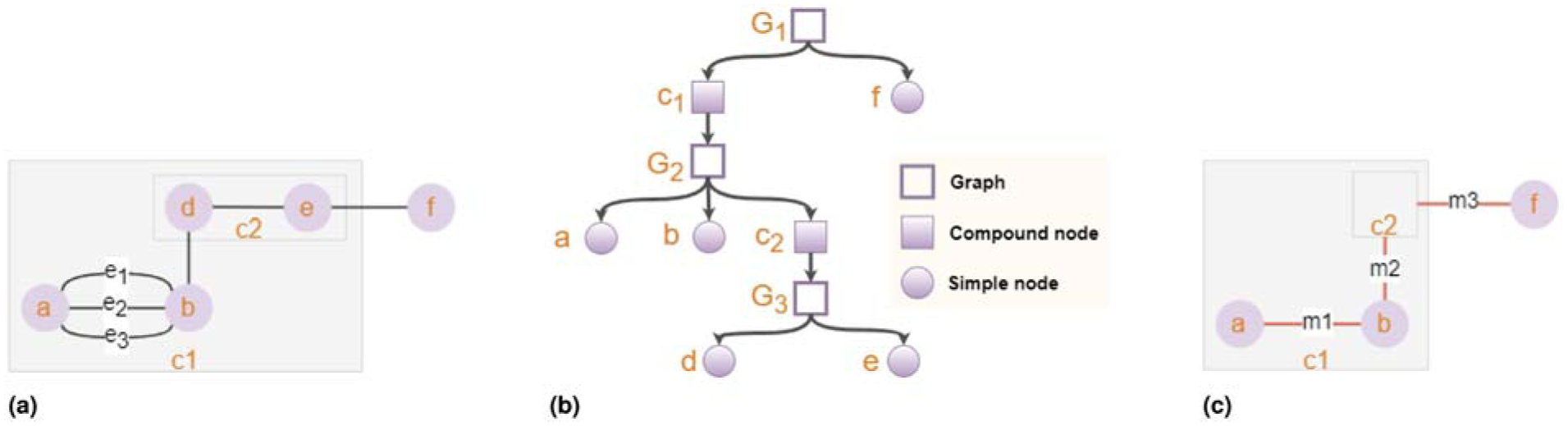A key distinction between a compound graph and related variants, such as hierarchically clustered graphs, is that the former allows edges to connect with its compound nodes, while the latter does not. Compound graphs are employed to depict different levels of groupings or abstractions in data, ¹⁰ and are particularly useful for managing complexity through the use of expand-collapse operations ⁸ (Figure 1).

Figure 1.

(a) A compound graph $G=(V,E,F)$ , where $V=\{a,b,d,e,f,c1,c2\}$ , $E=\{e_1=\{a,b\},e_2=\{a,b\},e_3=\{a,b\},\{b,d\},\{d,e\},\{e,f\}\}$ and $F=\{(c_1,a),(c_1,b),(c_2,d),(c_2,e),(c_1,c_2)\}$ , containing two compound nodes $c_1$ and $c_2$ and two inter-graph edges $\{b,d\}$ and $\{e,f\}$ , (b) its inclusion tree or nesting hierarchy, and (c) the same compound graph where the compound node $c2$ and multi-edges $e_1$ , $e_2$ and $e_3$ were collapsed and since some original edges are collapsed or no longer have both ends in the graph, they are represented with proxies called meta edges $m_1$ , $m_2$ and $m_3$ .

An induced graph $G^{\prime }=G[V^{\prime }]$ of a graph $G=(V,E)$ is a sub-graph of $G$ whose node set is $V^{\prime }\subseteq V$ and edge set is all edges whose both ends are in $V^{\prime }$ .

Graphs are typically presented using pictorial representations.^2,11,12 A poorly laid-out graph may lead to confusion for the user, whereas a well-organized one can provide aesthetic appeal and enhance the user’s comprehension of the underlying data. While the criteria for a good layout may be subjective, some generally accepted criteria include minimizing the number of edge-to-edge crossings, minimizing the total edge length, maintaining uniform edge length throughout the graph, and minimizing the drawing area. ¹³

In the context of interactive visual data analysis, any graph with a non-trivial size (more than several nodes and several edges) requires automatic layout, and any graph greater than about a hundred nodes and a similar number of edges is considered “large,” requiring some sort of complexity management to enable effective analysis.^14,15 The complexity of any graphs larger than this should be reduced on the server side or through appropriate filtering/querying operations to the associated knowledge base.

Related work

The most popular and easily implemented layout algorithms for graphs are force-directed algorithms, also known as spring embedders. These algorithms simulate a physical system that follows the fundamental laws of physics. Nodes in the graph are treated as particles with the same electrical charge, causing them to repel each other when they are too close. Meanwhile, edges in the graph are modeled as springs that attract their endpoints when they are too far apart.^13,16 The objective of these algorithms is to iteratively move the particles towards a stable state, where all forces balance out or the energy of the system is minimized. Many force-directed algorithms use a temperature, which is a variation of the simulated annealing technique, to help the algorithm quickly reach a local minimum of the energy function. fCoSE is an example of a force-directed layout algorithm that supports compound nodes. ¹⁷

Graphs that alter over time are frequently used in interactive visualization applications; this necessitates an adjusted layout. Incremental layout is the method of calculating a new layout while taking into account any current locations.^13,18 An incremental layout aims to clean up the drawing while maintaining the user’s mental map, which alludes to the nodes’ present locations. The similarity of two graphs using orthogonal ordering (relative positions of the nodes about each other within the layout) and neighborhood proximity (a measure of separation between nodes within the layout) has been used in the past to measure the success of an incremental layout algorithm. ¹⁹

The need to view ever-larger sets of relational data has increased the demand for more sophisticated complexity management methods. The complexity management issue in the setting of large graphs has been the subject of some studies.^7,8,20–26 Unwanted information can be concealed or ghosted and subsequently revealed upon request, using simple hide/show or more sophisticated semantic zooming techniques.^27,28 Some methods^29,30 make use of lenses, such as fisheye lenses, which enlarge a particular area of the drawing to enable users to zoom in on a particular area of a vast network. Others,^31,32 which support multiple views and nesting and use aggregation or expand-collapse operations to manage complexity, rely on techniques for building clusters. Such techniques are based on the node/link attributes or the graph-theoretic properties of the given dataset, if not any domain-specific information. Various edge bundling and edge collapsing strategies^33–35 have also been developed to specifically address the complexity caused by dense and overlapping edges in graph visualizations, helping to reduce visual clutter and making the underlying structure and relationships in the data easier to understand.

In-depth studies on complexity management often fail to address implementation concerns, such as preserving the user’s mental map when modifications are made to the graph’s topology and geometry. More importantly, when used in combination and applied in a specific order, these complexity management methods will operate independently, leading to potential inconsistencies, incorrect behaviors (see the section titled Motivation in the Supplemental Material), and inefficient utilization of computing resources.

With respect to existing tools and libraries, only a few commercial products—such as Tom Sawyer Perspectives, ³⁶ Linkurious, ³⁷ and yFiles ³⁸ —support compound structures and expand/collapse functionality. However, these tools do not provide built-in support for other complexity management operations like hide/show or filter/unfilter, leaving their implementation to the end user, which is not straightforward at all. On the other hand, free tools such as Graphviz, ³⁹ Gephi, ⁴⁰ Tableau, ⁴¹ and D3 ⁴² generally lack support for complexity management operations, including compound structures or expand/collapse. Cytoscape.js is the only free library that offers support for compound structures as well as features like expand/collapse and hide/show. However, these complexity management operations rely on external extensions, ⁴³ which suffer from numerous reported bugs and issues, and are no longer maintained by their original authors.

Framework

We designed a framework named CMGV to solve the aforementioned problems in complexity management. It mainly consists of the following components (Figure 2):

• A graph model (CMGM) that will unify various complexity management techniques and allow them to work together seamlessly, and comes with specialized layout algorithms protecting the user’s mental map after each complexity management operation is applied.

• A complexity management extension (EXT) specific to the library (RL) that renders/displays users’ graphs.

• A specific rendering library (RL).

The details of the low-level architecture of CMGV can be found in the Supplementary.

Figure 2.

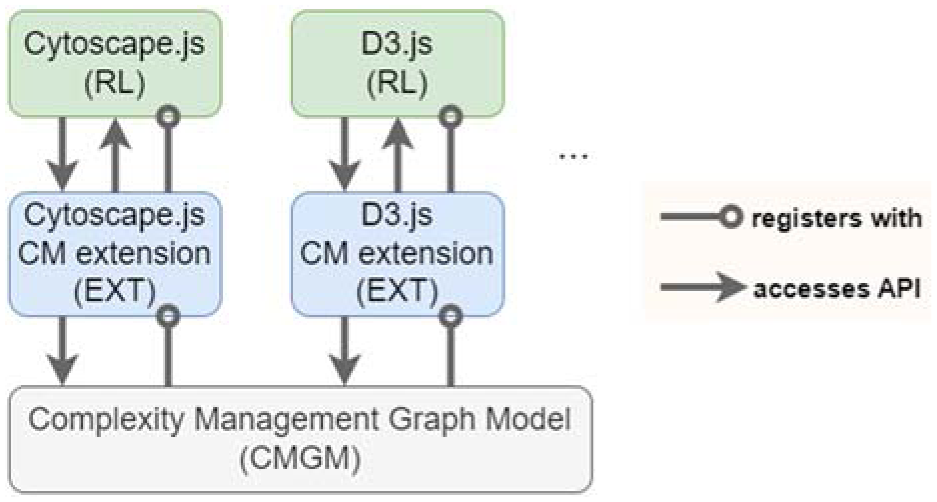
A diagram summarizing the architecture of an application using our CMGV framework.

A unified graph model

We first present a novel complexity management graph model (CMGM) that will support three kinds of most commonly used complexity management operations on graph elements:

• filter / unfilter a set of graph objects based on one or more of their properties,

• hide / show a set of graph objects specified by the user, and

• collapse / expand contents (i.e., child graph) of a compound node or multiple edges between a pair of nodes.

CMGM is designed to be rendering layer-independent, allowing its use with varying graph rendering libraries (RLs). A graph on the renderer’s side will be represented with two compound graphs in CMGM, isolating the viewable graph in the rendering library, and avoiding any potential interference with what the user actually sees. One of these graphs, called the visible graph, is for only the currently visible graph elements, and the other one, called the main graph, is for all, including the invisible elements that are removed temporarily due to complexity management operations. This is the popular model-view architecture in action, where the main graph forms a model for the two view graphs (the visible graph in CMGM and the graph rendered by RL). This might come at an additional cost, but it is necessary to clearly separate what is visible from what the original topology is.

Each of the compound graphs in CMGM is managed by a graph manager object based on graph managers in. ⁷ A graph manager manages individual graphs (i.e., the root graph and the graphs nested within any compound nodes) as well as the inter-graph edges between them (see the class diagram in Figure 10 of the Supplemental Material).

We assume that communication between RL and CMGM is facilitated via an extension (EXT) of RL, ensuring the necessary flow of information and synchronization of their respective graphs (Figure 2). Changes initiated by a user, such as topology modifications or complexity management operations, are reflected in both views through the model-view architecture. This communication occurs via the associated EXT, utilizing the API provided by the CMGM, as detailed in the Supplementary. Maintaining separate graphs for RL and CMGM necessitates that changes made in one are promptly mirrored in the other to ensure synchronization of operations and structures, underscoring the importance of establishing a consistent communication structure between the two graph models.

The CMGM architecture, together with further details of the proposed operations and sample scenarios, and the communication structure between RL and CMGM are detailed in the Supplemental Material.

Complexity management operations

As listed earlier, our framework supports three kinds of complexity management operations. Most of these operations (filter/unfilter and hide/show) solely require making a graph element visible or invisible in the RL graph view by changing its visibility, which may, in turn, be based on their filtered and hidden statuses. Applying expand/collapse operations, however, might require the use of so-called meta edges, a proxy representation of an edge that can not be directly represented in the visible graph. Hence, we focus on these operations in the context of the creation and destruction of meta edges in the remainder of this section.

We use three separate hash maps (nodes, edges, and meta-edges maps) to easily map IDs to objects and keep track of a respective graph element with a common ID in other graph models. Additionally, there is a fourth hash map called the edgeToMetaEdgeMap, which tracks all edges by their parent meta edge ID.

Collapsing nodes or edges

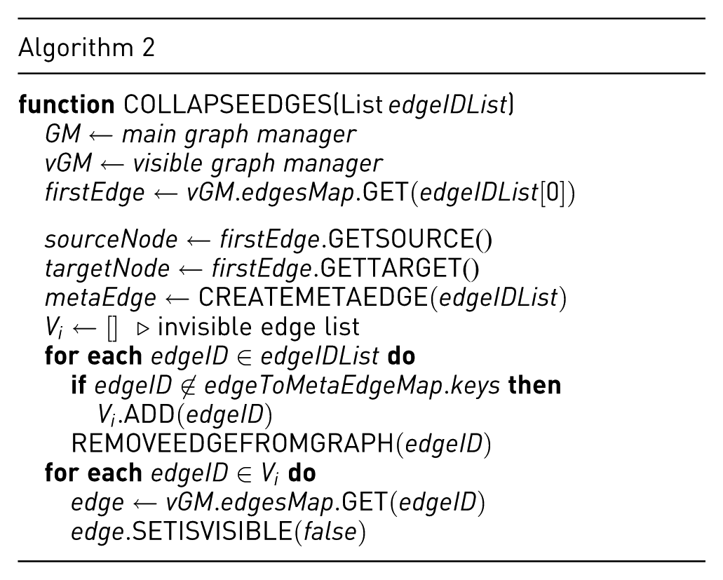
There are two ways for meta edges to be created. The first is edge collapse, where multiple edges between the same pair of nodes are collapsed into a single so-called meta edge. The second way, on the other hand, is node collapse, where a compound node is collapsed and its contents (child graph) are no longer viewable. Since the collapse node operation removes child nodes of the collapsing compound from the visible graph, either the source or target node of an inter-graph edge with exactly one end in the collapsing node is bound to be removed; thus, a meta edge is created as a proxy representation between the compound node and the original end node outside the collapsing compound (see Figures 1 and 3 for examples).

In our framework, every meta edge maintains an original edge list containing the IDs of all the edges that it represents. Considering a meta edge as a parent and the edges it represents as its children, which in turn may be other meta edges, results in some kind of an ancestry relationship, which we call a meta edge lineage (see Figure 3 for examples). Note that an original edge list will be of length one for all meta edges created due to a node collapse operation (one per each inter-graph edge) and of length at least two in the case where the meta edge is created on an edge collapse operation. This distinction in the length of the original edges list may be explicitly used in the implementation to differentiate a node collapse meta edge from the others in a meta edge lineage.

An exception to the rule of creating a new meta edge for an inter-graph edge may happen during node collapse. If a meta inter-graph edge for which a new meta edge is to be created is encountered, an optimization measure is taken, and instead of creating a new meta edge, either the source or target of the existing meta edge is changed to be the collapsing node. This is done to reduce both the number of meta-edges created and the length of meta-edge lineages.

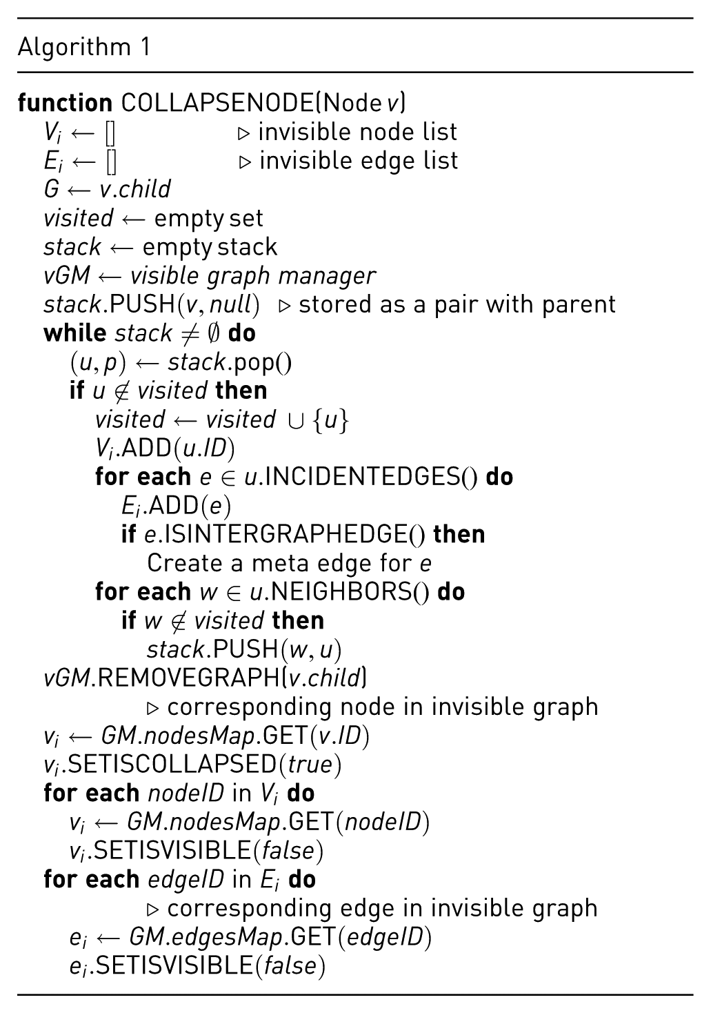
The collapse node algorithm (Algorithm 1) iterates over each child node and then their respective edges, removing them from the graph and introducing meta edges as needed. This is accomplished through a BFS-based traversal that recursively identifies all graph content contained within the collapsed node $v$ , and creates meta edges as inter-graph links connecting elements outside of $v$ . Finally, hash maps are updated to maintain associations. Both the removal and the meta edge creation can be completed in constant time per graph object. Hence, the overall expected runtime complexity of this operation is linear in the number of nodes and edges involved ( $O(\left|V\right|+\left|E\right|)$ ). The algorithm to collapse a group of multi-edges between a node pair will also work locally with associated edges (Algorithm 2). Hence, the runtime complexity is expected to be linear with respect to the number of edges involved ( $O\left(\left|E\right|\right)$ ).

Algorithm 1

function COLLAPSENODE( $\mathrm{Node}v$ )   $V_i\leftarrow []▹$ invisible node list   $E_i\leftarrow []▹$ invisible edge list   $G\leftarrow v.\mathrm{child}$   $\mathrm{visited}\leftarrow \mathrm{empty}\mathrm{set}$   $\mathrm{stack}\leftarrow \mathrm{empty}\mathrm{stack}$   $\mathrm{vGM}\leftarrow$ visible graph manager   $\mathrm{stack}.\mathrm{PUSH}(v,\mathrm{null})▹$ stored as a pair with parent  while $\mathrm{stack}\ne \varnothing$ do    $(u,p)\leftarrow \mathrm{stack}.\mathrm{pop}()$   if $u\notin \mathrm{visited}$ then     $\mathrm{visited}\leftarrow \mathrm{visited}\cup \{u\}$     $V_i.\mathrm{ADD}(u.\mathrm{ID})$    for each $e\in u.\mathrm{INCIDENTEDGES}()$ do      $E_i.\mathrm{ADD}\left(e\right)$     if $e.\mathrm{ISINTERGRAPHEDGE}()$ then      Create a meta edge for $e$    for each $w\in u.\mathrm{NEIGHBORS}()$ do     if $w\notin \mathrm{visited}$ then       $\mathrm{stack}.\mathrm{PUSH}(w,u)$   $\mathrm{vGM}$ .REMOVEGRAPH( $v.\mathrm{child}$ )      ▹ corresponding node in invisible graph   $v_i\leftarrow \mathrm{GM}.\mathrm{nodesMap}.\mathrm{GET}(v.\mathrm{ID})$   $v_i.\mathrm{SETISCOLLAPSED}\left(\mathrm{true}\right)$  for each $\mathrm{nodeID}$ in $V_i$ do    $v_i\leftarrow \mathrm{GM}.\mathrm{nodesMap}.\mathrm{GET}\left(\mathrm{nodeID}\right)$    $v_i.\mathrm{SETISVISIBLE}\left(\mathrm{false}\right)$  for each $\mathrm{edgeID}$ in $E_i$ do      ▹ corresponding edge in invisible graph    $e_i\leftarrow \mathrm{GM}.\mathrm{edgesMap}.\mathrm{GET}\left(\mathrm{edgeID}\right)$    $e_i.\mathrm{SETISVISIBLE}\left(\mathrm{false}\right)$

Algorithm 2

function COLLAPSEEDGES( $\mathrm{List}\mathrm{edgeIDList}$ )   $\mathrm{GM}\leftarrow$ main graph manager   $\mathrm{vGM}\leftarrow$ visible graph manager   $\mathrm{firstEdge}\leftarrow \mathrm{vGM}.\mathrm{edgesMap}.\mathrm{GET}(\mathrm{edgeIDList}[0])$   $\mathrm{sourceNode}\leftarrow \mathrm{firstEdge}.\mathrm{GETSOURCE}()$   $\mathrm{targetNode}\leftarrow \mathrm{firstEdge}.\mathrm{GETTARGET}()$   $\mathrm{metaEdge}\leftarrow \mathrm{CREATEMETAEDGE}\left(\mathrm{edgeIDList}\right)$   $V_i\leftarrow []▹$ invisible edge list  for each $\mathrm{edgeID}\in \mathrm{edgeIDList}$ do   if $\mathrm{edgeID}\notin \mathrm{edgeToMetaEdgeMap}.\mathrm{keys}$ then     $V_i.\mathrm{ADD}\left(\mathrm{edgeID}\right)$    $\mathrm{REMOVEEDGEFROMGRAPH}\left(\mathrm{edgeID}\right)$  for each $\mathrm{edgeID}\in V_i$ do    $\mathrm{edge}\leftarrow \mathrm{vGM}.\mathrm{edgesMap}.\mathrm{GET}\left(\mathrm{edgeID}\right)$    $\mathrm{edge}.\mathrm{SETISVISIBLE}\left(\mathrm{false}\right)$

Expanding nodes or edges

Expand node operation, which is the reversal of the collapse node operation, starts by bringing back all the child nodes of the expanding compound node to the visible graph unless they are filtered or hidden. Keep in mind that an edge will only become visible if both ends are expanded, and the edge itself is neither filtered nor hidden, under the assumption that all three types of operations function in sync. This is followed by bringing back and making visible any intra-graph edges between newly visible child nodes, again assuming they are not filtered or hidden. To reverse the creation of meta edges during the matching collapse operation, such meta edges need to be destroyed, any references to them need to be removed, and corresponding original edges need to be restored.

To accomplish these tasks and achieve the desired result, we first need to determine the current standing of the edge we are processing. Only the edges not in the visible graph, which are inter-graph edges with source/target outside the expanding node, can be part of any node collapse meta-edges. Thus, we begin by finding and filtering out any edges meeting these criteria and destroying them.

As we established in the previous section, a meta edge can potentially be part of a meta edge lineage; so when we destroy a meta edge, we must remove all its instances from the lineage as well. In order to do that, we must pinpoint the node collapse meta edge in the lineage, by starting from the simple edge and going upwards from its parent to its parent’s parent and so on and so forth, until we find a meta edge whose original edges list only contains a single edge. For future reference, let’s call such an edge a target meta edge. Then, we start by removing the target meta edge from the lineage and divide it into two; the first lineage will begin from the child of the target meta edge, and the second one will end at the parent of the target meta edge. The second lineage will need a slight reconfiguration after the loss of a member. One of the following can happen:

1. The target meta edge has no parent (i.e., a single-member lineage).

2. The target meta edge has a parent with only two children; with one gone, the parent meta edge is unnecessary. When this is the case, the sibling of the target meta edge becomes part of its grandparent’s original edge list. If there are none, then it will be a single-member lineage.

3. The target meta edge has multiple siblings. Then, the lineage reconfiguration is unnecessary.

After reconfiguration, we destroy the target meta edge and bring back the top meta edges of both lineages to the visible graph (assuming they are not filtered or hidden).

To bring any edge back to the visible graph, both its source and target nodes need to be visible. Hence, when exactly one end node is not visible, we create a new meta edge between the visible end node and the visible parent of the invisible end node, and add the edge to the original edges list of our new meta edge. Where both end nodes are invisible, a new meta edge is created between each end node’s lowest visible ancestor in the nesting hierarchy.

To expand a compound node by making its child graph visible and updating the relevant meta edge accordingly, we iterate over each child node and then their respective edges, making them visible (Algorithm 3). This is done by simply checking each direct or indirect child of the expanded node to determine whether it should be visible, as previously explained in this section. The algorithm is expected to have a runtime complexity linear in the number of graph objects involved since the expand node function traverses over all children nodes and edges and makes them visible. Hence, the worst-case runtime complexity is $O(\left|V\right|+\left|E\right|)$ . Similarly, Algorithm 4 is a function to expand a meta edge by making the original edges visible depending upon their filter and hidden status. As stated, the function iterates over all the edges that are part of the expanding meta edge; hence, the runtime complexity is expected to be linear with respect to the number of edges ( $O\left(\left|E\right|\right)$ ).

Algorithm 3 Takes whether or not it should recursively continue as a parameter

function EXPANDNODE( $\mathrm{Node}v,\mathrm{bool}\mathrm{isRec}$ )   $\mathrm{GM}\leftarrow$ main graph manager   $\mathrm{vGM}\leftarrow$ visible graph manager    ▹ corresponding node in invisible graph   $v_i\leftarrow \mathrm{GM}.\mathrm{nodesMap}.\mathrm{Get}(v.\mathrm{ID})$   $\mathrm{emptyGraph}=\mathrm{vGM}.\mathrm{NEWGRAPH}()$   $\mathrm{vGM}.\mathrm{ADDGRAPH}(\mathrm{emptyGraph},v)$   $v.\mathrm{child}.\mathrm{sibling}\leftarrow v_i.\mathrm{child}$   $v_i.\mathrm{child}.\mathrm{sibling}\leftarrow v.\mathrm{child}$   $\mathrm{childrenNodes}\leftarrow \mathrm{GETDESCENDANTSINORDER}\left(v\right).\mathrm{NODES}()$    ▹ a sorted (from topmost parent to simple nodes in the nesting hierarchy) list of descendants   $\mathrm{markedChildren}\leftarrow []$  for each $c\in \mathrm{childrenNodes}$ do  if $(!c.\mathrm{isFiltered}\wedge !c.\mathrm{isHidden}\wedge !c.\mathrm{isCollapsed})\vee$   $(c.\mathrm{isFiltered}\wedge !c.\mathrm{isHidden}\wedge c.\mathrm{isCollapsed}\wedge \mathrm{isRec})$ then   $\mathrm{reportedEdges}\leftarrow \mathrm{moveNodeToVisible}\left(v\right)$    ▹ report all edges (to be removed) and meta edges (to be removed & to be added) to renderer side using global variables   if $c.\mathrm{child}$ then     $\mathrm{EXPANDNODE}(c,\mathrm{isRec})$   else if $!c.\mathrm{isFiltered}\wedge !c.\mathrm{isHidden}\wedge c.\mathrm{isCollapsed}\wedge !\mathrm{isRec}\mathbf{then}$    $\mathrm{reportedEdges}\leftarrow \mathrm{MOVENODETOVISIBLE}\left(v\right)$    ▹ report child node, all edges, and meta edges to renderer side using global variables.    $\mathrm{markedChildren}.\mathrm{add}\left(c\right)$  for each $u\in \mathrm{markedChildren}$ do   for each $e\in u.\mathrm{INCIDENTEDGES}()$ do    if $e\in \mathrm{GM}.\mathrm{edgeToMetaEdgeMap}.\mathrm{keys}$ then     $m\leftarrow \mathrm{GETTOPMETAEDGE}\left(e\right)$     ▹ check if an end node of $m$ is an end node     ▹ of any of the child edges     $E_i\leftarrow v.\mathrm{child}.\mathrm{INCIDENTEDGES}()$    if $\{w|w=m.\mathrm{source}\wedge (w=x\vee w=y)\wedge \{x,y\}\in E_i\}\vee \{w|w=m.\mathrm{target}\wedge (w=x\vee w=y)\wedge \{x,y\}\in E_i\}$ then     if $m.\mathrm{source}.\mathrm{owner}=m.\mathrm{target}.\mathrm{owner}$ then      ▹ source and target as before       $m.\mathrm{source}.\mathrm{owner}.\mathrm{ADDEDGE}\left(m\right)$     else      ▹ source and target as before       $\mathrm{GM}.\mathrm{ADDINTERGRAPHEDGE}\left(m\right)$      ▹ report $m$ (to be added) to renderer side using global variables

Algorithm 4 Takes edges to be expanded and whether or not it should recursively continue

function EXPANDEDGES( $\mathrm{List}\mathrm{edgeIDList},\mathrm{bool}\mathrm{isRec}$ )   $\mathrm{GM}\leftarrow$ main graph manager   $\mathrm{vGM}\leftarrow$ visible graph manager  for each $\mathrm{ID}\in \mathrm{edgeIDList}$ do    $M\leftarrow \mathrm{vGM}.\mathrm{edgeToMetaEdgeMap}.\mathrm{get}\left(\mathrm{ID}\right)$    $S\leftarrow M.\mathrm{GETSOURCE}()$    $T\leftarrow M.\mathrm{GETTARGET}()$   for each $e\in M.\mathrm{orignalEdgesList}$ do    if $e.\mathrm{ID}\in \mathrm{vGM}.\mathrm{metaEdgeMap}.\mathrm{keys}$ then     if $S.\mathrm{owner}$ = $T.\mathrm{owner}$ then       $S.\mathrm{owner}.\mathrm{ADDEDGE}(e,S,T)$     else       $\mathrm{vGM}.\mathrm{ADDINTERGRAPHEDGE}(e,S,T)$     if $\mathrm{isRec}\mathbf{then}$       $\mathrm{EXPANDEDGES}(e.\mathrm{ID},\mathrm{isRec})$   else     $e_i\leftarrow \mathrm{GM}.\mathrm{edgesMap}..\mathrm{get}(e.\mathrm{ID})$    if ! $e_i.\mathrm{isFiltered}\wedge !e_i.\mathrm{isHidden}$ then      $e_i.\mathrm{setIsVisible}\left(\mathrm{true}\right)$    if $S.\mathrm{owner}=T.\mathrm{owner}$ then      $S.\mathrm{owner}.\mathrm{ADDEDGE}(e,S,T)$    else      $\mathrm{vGM}.\mathrm{ADDINTERGRAPHEDGE}(e,S,T)$

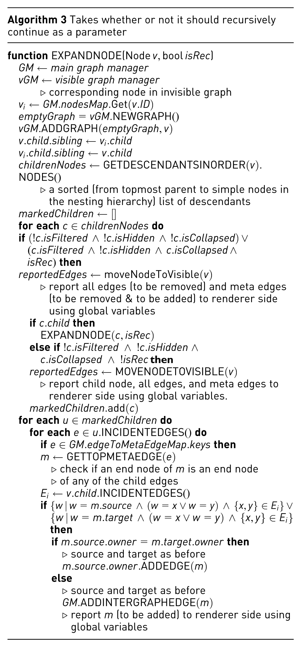
Figure 3 shows a sample scenario, where a series of mixed node and edge collapse/expand operations are performed, to illustrate how the internal representation changes as the operations take place. Below is the notation we use for this purpose:

Figure 3.

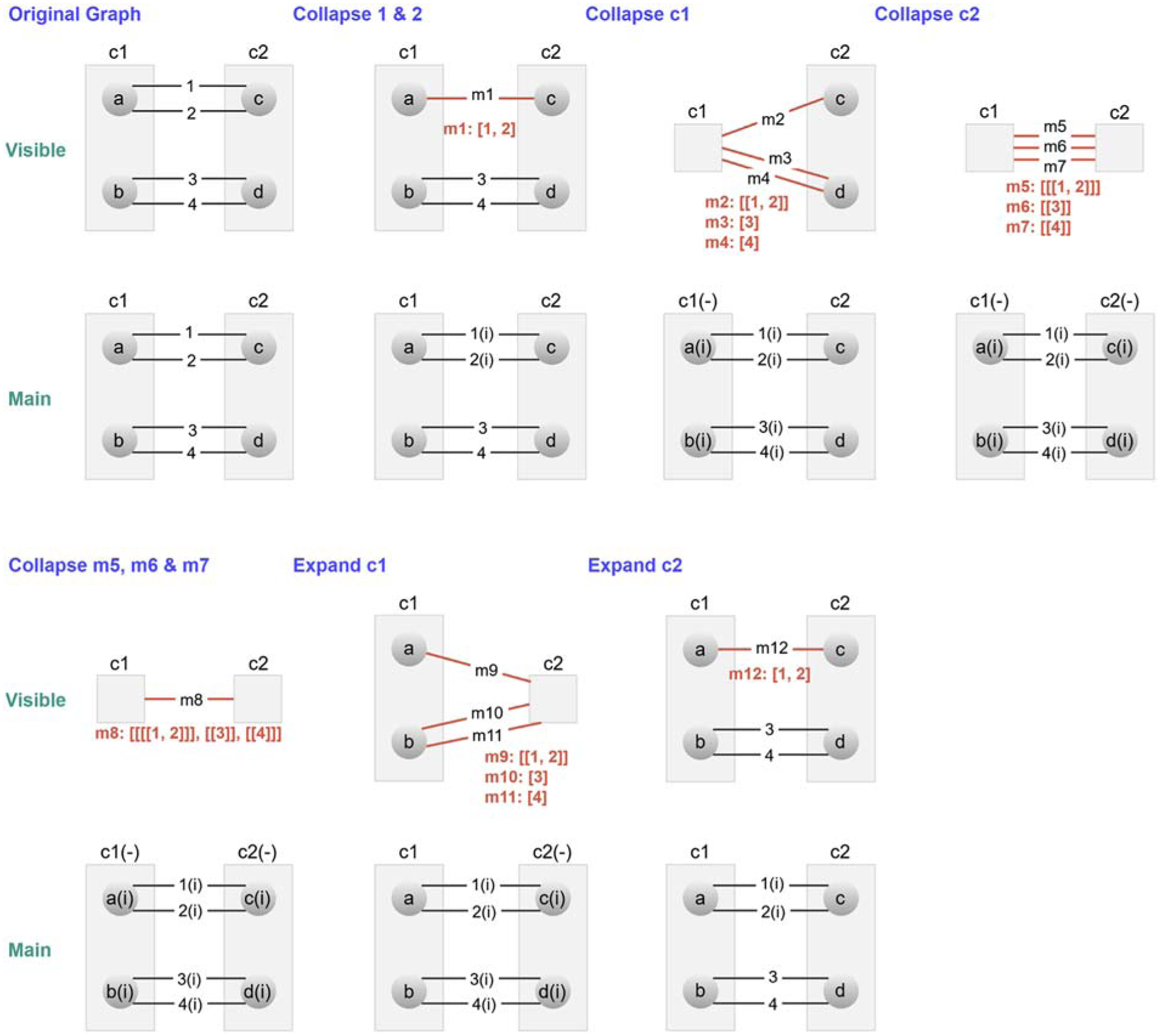
A series (from left to right and top to bottom) of mixed node and edge collapse/expand operations. Notice how visible and main graph models, as well as any meta-edge lineages (in red), change.

• $a,b,c,\dots$ : simple nodes

• $c1,c2,\dots$ : compound nodes

• $1,2,3,\dots$ : simple edges

• $m1,m2,\dots$ : meta edges

• $\left(i\right)$ : invisible (isVisible = false)

• $\left(f\right)$ : filtered (isFiltered = true)

• $\left(h\right)$ : hidden (isHidden = true)

• (−): collapsed (isCollapsed = true)

• $[1]$ , $[[1]]$ , …: meta edge experienced one, two,…consecutive node collapses

• $[1,2]$ : meta edge generated via collapse of edges $1$ and $2$

Note here that if there is only one element inside square brackets, it corresponds to a node collapse. If there are more elements, however, the associated elements must have gone through an edge collapse. For example, $m1:[[[1,2],3]]$ implies that there were three edges numbered $1$ , $2$ , and $3$ between their source and target nodes, and first, edges 1 and 2 were collapsed, resulting in a meta edge $[1,2]$ . Then two edges $[1,2]$ and $3$ were collapsed, creating a new meta edge $[[1,2],3]$ . Lastly, either the source or target node of the meta edge $[[1,2],3]$ was collapsed, resulting in the meta edge $[[[1,2],3]]$ .

The Supplemental Material presents further scenarios to illustrate how the CMGM graph models change as a combination of various complexity management operations is applied.

Methods

It is imperative that, as complexity management operations take place, the user’s mental map is not destroyed, impairing the analysis. Furthermore, the layout algorithm used by the complexity management operations should produce compatible/consistent results with the base layout algorithm used by the application. This base algorithm should support compound structures and incremental layout, and should be easily customizable for adjusting layout during complexity management operations. For our work, we chose fCoSE ¹⁷ as our base layout algorithm since it satisfies the aforementioned requirements.

Some complexity management operations may be handled using the base layout algorithm in incremental mode, where the current respective positions of graph elements are maintained. In the case of force-directed layout algorithms such as fCoSE, this simply corresponds to starting the iterative algorithm from the current node positions, instead of randomly placing them. Adjustment of the layout after a collapse operation is exemplified in Figure 4. However, the expand node and show/unfilter operations require specialized incremental layout algorithms to ensure newly introduced, possibly large content, does not overlap and, hence, tangle surrounding graph elements, tarnishing the existing nice layout. An expand operation in the middle of the nesting hierarchy of multiply nested compound structures makes things even more difficult.

Figure 4.

A sample layout adjustment on a collapse operation (a) original visible graph (b) visible and (c) main graphs after collapsing $n29$ (blue in visible graph; its direct and indirect children nodes are no longer visible, depicted as ghosted) (d) visible graph after applying an incremental base layout; unnecessary space around collapsing node is eliminated.

Adjusting layout on expand

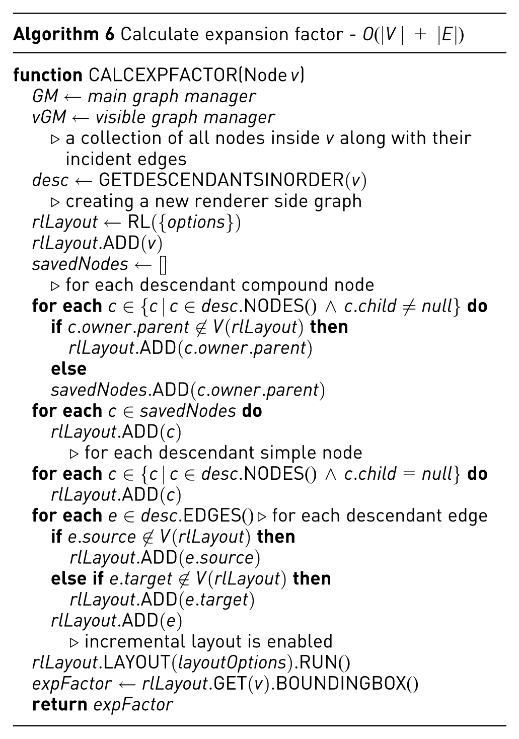
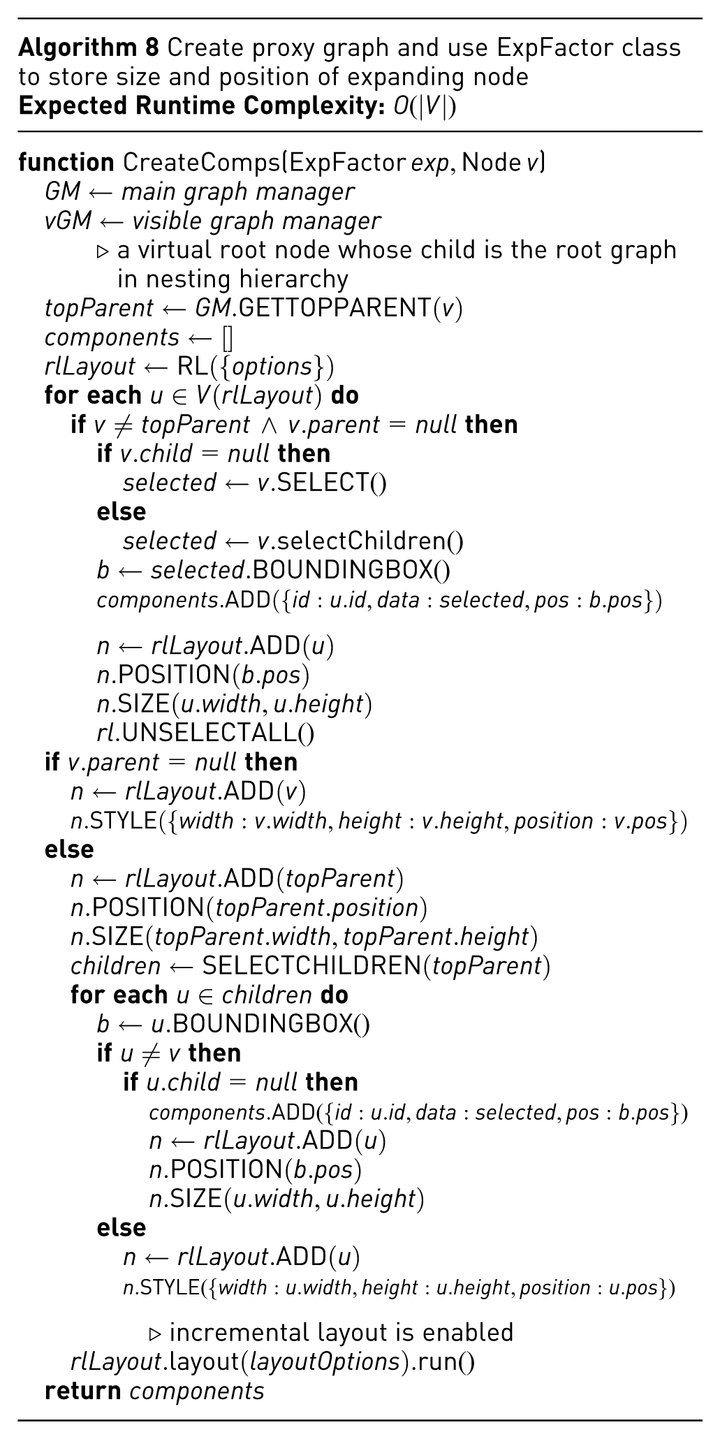
Our base layout fCoSE was customized with a post-processing step for the expand operation as follows. The main idea here is to estimate the amount of additional space needed by the expanding node and create a “proxy graph” with just the main components of the visible graph, with appropriate node dimensions and no edges. In other words, the proxy graph consists of one node per component of the main graph, and two nodes $u$ and $v$ in the proxy graph are connected if and only if there exists an edge from a node in the component represented by $u$ to a node in the component represented by $v$ . Then the base layout is applied to this proxy graph in incremental mode, making enough room for the expanding node before the actual expansion takes place. A subsequent incremental layout tidies up the layout of the whole graph with expanded contents. An example is provided in Fig. 5. More formally, for a compound graph $G=(V,E,F)$ with an expanding node $u\in V$ , we first estimate the size of $u$ after expansion. To do so, an induced immediate neighborhood or simply neighborhood sub-graph $G^N$ of $G$ containing the expanding node and its contents along with immediate neighbors of $u$ itself and its children that are outside $u$ is computed (i.e., inter-graph edges connecting $u$ or its contents to outside $u$ ). Specifically, $G^N=G[V^N]$ is an induced subgraph of $G$ on $V^N$ , where

$$\begin{array}{c}{V}^{N_0}=\{v|\{v_0=u,v_1,\dots v_k=v\}\subseteq V\left(G\right)\wedge k\ge 0\hfill \\ \multicolumn{1}{c}{\wedge (0<i\le k-1)\Rightarrow \{v_i,v_{i+1}\}\in E\left(F\right)\},\mathrm{and}}\\ \multicolumn{1}{c}{V^N=V^{N_0}\cup \{v|v\in V\left(G\right)\setminus V^{N_0}\wedge }\\ \multicolumn{1}{c}{\{u,v\}\in E\left(G\right)\mathrm{is}\mathrm{an}\mathrm{inter}-\mathrm{graph}\mathrm{edge}\}.}\end{array}$$

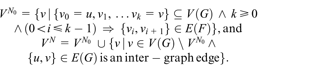
We then lay out $G^N$ incrementally. The dimensions of $u$ after this layout step should be a decent estimate of the expanding node after the expansion. Notice here that we refrain from laying out the entire graph as it might be costly timewise (see Figure 5(b)). Then, we construct a proxy graph $G^P=(V^P,\{\})$ where

$$\begin{array}{c}{V}^P=\{v^P|v^P\mathrm{represents}\mathrm{a}\mathrm{root}\mathrm{graph}\mathrm{node}v\in V\left(G\right)\hfill \\ \multicolumn{1}{c}{\wedge v\in V\left(G\right)-\{u\}\Rightarrow \dim \left(v^P\right)=\dim \left(v\right)}\\ \multicolumn{1}{c}{\wedge u\in V\left(G\right)\Rightarrow \dim \left(u^P\right)=\dim \left(u^X\right)\},}\end{array}$$

and $\dim \left(u^X\right)$ is the estimated dimension of $u$ after expansion as explained earlier.

Figure 5.

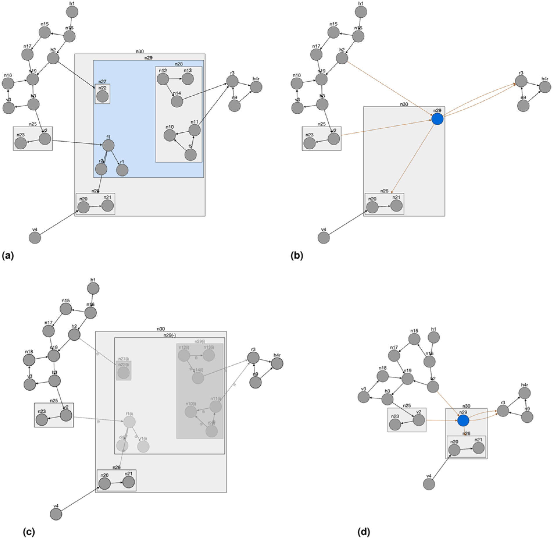
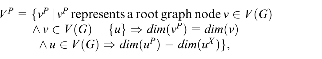
A sample layout adjustment on an expand operation (a) an original visible graph without any layout adjustment after expanding n29 in the graph of Figure 4(d) (notice how expanded content tangles the surrounding graph objects; some graph objects stay behind compound boxes) (b) an incremental layout of the immediate neighborhood graph (notice how nonimmediate neighbors such as h3 are excluded in this stage) used to estimate expanding node's size after expansion (c) proxy graph after an incremental layout (d) visible graph after graph components are repositioned based on the layout of the proxy graph (e) expanded visible graph before a final incremental layout is applied, and (f) final layout, after which node separation and edge lengths become more uniform.

An incremental layout of $G^P$ now will provide us with what locations the main components of the original graph $G$ should start from, on a final incremental layout. Once again, the proxy graph is typically much smaller than the original graph, saving time on the task of adjusting the layout (see Figure 5c).

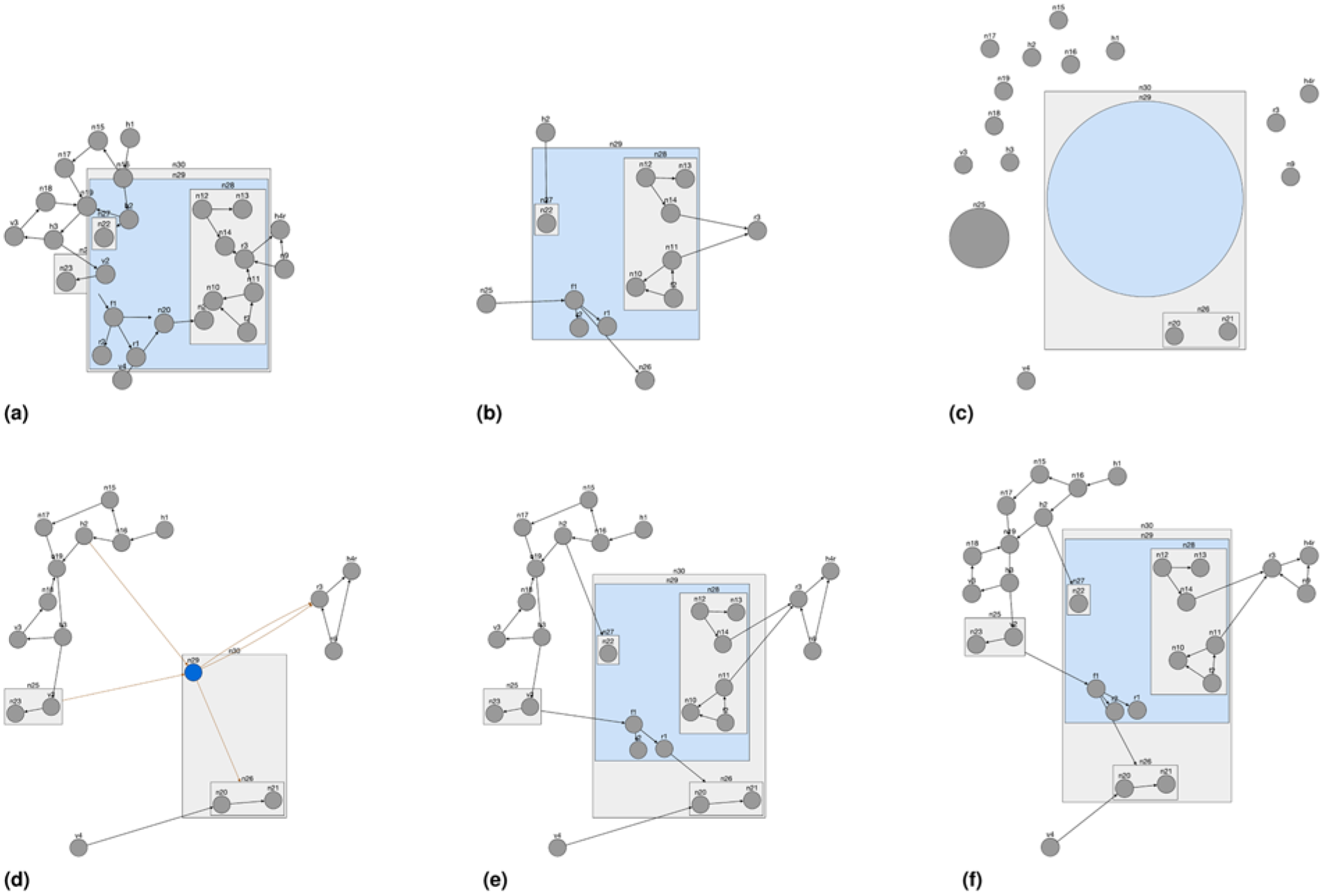
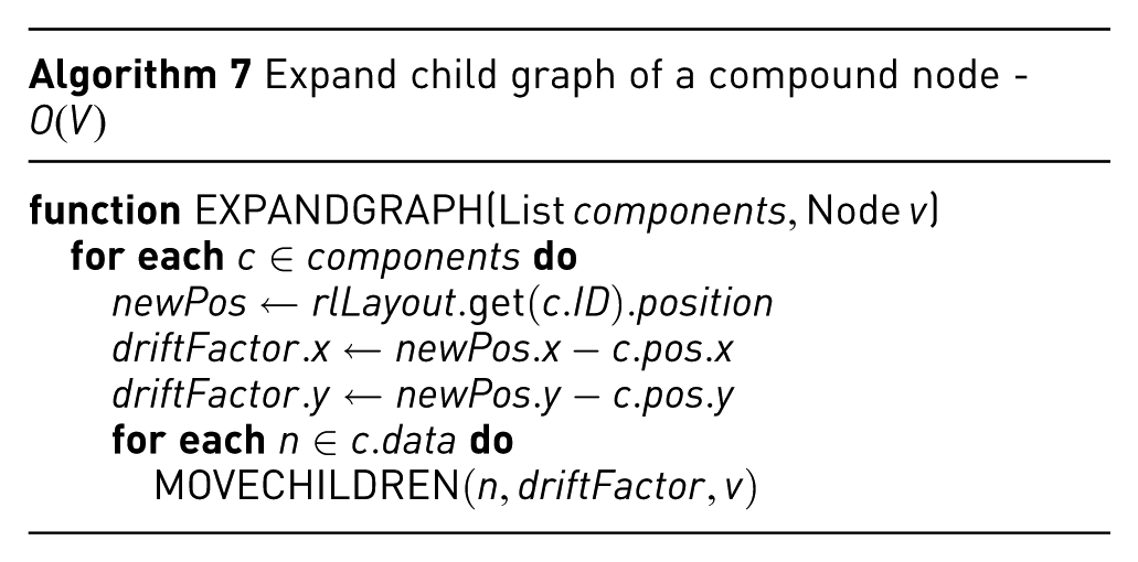
After the nodes of the proxy graph representing the components of the original graph are finalized, we move the compounds of the original graph to those positions suggested by the proxy graph (see Figure 5d and 5e). Lastly, a final incremental layout polishes the drawing (see Figure 5f). Algorithms 5 through 7 provide the pseudocode for the expand node operation, including the customized layout calculations. $\mathrm{CREATECOMPS}$ invoked here is detailed in Algorithm 8.

Algorithm 5
function EXPANDNODEWITHLAYOUT( $\mathrm{Node}v$ )   $\exp \leftarrow \mathrm{CALCEXPFACTOR}\left(v\right)$   $\mathrm{components}\leftarrow \mathrm{CREATECOMPS}(\exp ,v)$   $\mathrm{EXPANDGRAPH}(\mathrm{components},v)$   $\mathrm{EXPANDNODE}\left(v\right)$

Algorithm 6 Calculate expansion factor - $O(|V|+|E|)$

function CALCEXPFACTOR( $\mathrm{Node}v$ )   $\mathrm{GM}\leftarrow$ main graph manager   $\mathrm{vGM}\leftarrow$ visible graph manager   ▹ a collection of all nodes inside $v$ along with their incident edges   $\mathrm{desc}\leftarrow \mathrm{GETDESCENDANTSINORDER}\left(v\right)$   ▹ creating a new renderer side graph   $\mathrm{rlLayout}\leftarrow \mathrm{RL}(\{\mathrm{options}\})$   $\mathrm{rlLayout}.\mathrm{ADD}\left(v\right)$   $\mathrm{savedNodes}\leftarrow []$   ▹ for each descendant compound node  for each $c\in \{c|c\in \mathrm{desc}.\mathrm{NODES}()\wedge c.\mathrm{child}\ne \mathrm{null}\}$ do   if $c.\mathrm{owner}.\mathrm{parent}\notin V\left(\mathrm{rlLayout}\right)$ then    $\mathrm{rlLayout}.\mathrm{ADD}(c.\mathrm{owner}.\mathrm{parent})$   else    $\mathrm{savedNodes}.\mathrm{ADD}(c.\mathrm{owner}.\mathrm{parent})$  for each $c\in \mathrm{savedNodes}$ do    $\mathrm{rlLayout}.\mathrm{ADD}\left(c\right)$    ▹ for each descendant simple node  for each $c\in \{c|c\in \mathrm{desc}.\mathrm{NODES}()\wedge c.\mathrm{child}=\mathrm{null}\}$ do    $\mathrm{rlLayout}.\mathrm{ADD}\left(c\right)$  for each $e\in \mathrm{desc}.\mathrm{EDGES}()▹$ for each descendant edge   if $e.\mathrm{source}\notin V\left(\mathrm{rlLayout}\right)$ then     $\mathrm{rlLayout}.\mathrm{ADD}(e.\mathrm{source})$   else if $e.\mathrm{target}\notin V\left(\mathrm{rlLayout}\right)$ then     $\mathrm{rlLayout}.\mathrm{ADD}(e.\mathrm{target})$    $\mathrm{rlLayout}.\mathrm{ADD}\left(e\right)$    ▹ incremental layout is enabled   $\mathrm{rlLayout}.\mathrm{LAYOUT}\left(\mathrm{layoutOptions}\right).\mathrm{RUN}()$   $\mathrm{expFactor}\leftarrow \mathrm{rlLayout}.\mathrm{GET}\left(v\right).\mathrm{BOUNDINGBOX}()$  return $\mathrm{expFactor}$

Algorithm 7 Expand child graph of a compound node - $O(V)$

function EXPANDGRAPH( $\mathrm{List}\mathrm{components},\mathrm{Node}v$ )  for each $c\in \mathrm{components}$ do    $\mathrm{newPos}\leftarrow \mathrm{rlLayout}.\mathrm{get}(c.\mathrm{ID}).\mathrm{position}$    $\mathrm{driftFactor}.x\leftarrow \mathrm{newPos}.x-c.\mathrm{pos}.x$    $\mathrm{driftFactor}.y\leftarrow \mathrm{newPos}.y-c.\mathrm{pos}.y$   for each $n\in c.\mathrm{data}$ do     $\mathrm{MOVECHILDREN}(n,\mathrm{driftFactor},v)$

Algorithm 8 Create proxy graph and use ExpFactor class to store size and position of expanding nodeExpected Runtime Complexity: $O(|V|)$

function CreateComps( $\mathrm{ExpFactor}\exp ,\mathrm{Node}v$ )   $\mathrm{GM}\leftarrow$ main graph manager   $\mathrm{vGM}\leftarrow$ visible graph manager    ▹ a virtual root node whose child is the root graph in nesting hierarchy   $\mathrm{topParent}\leftarrow \mathrm{GM}.\mathrm{GETTOPPARENT}\left(v\right)$   $\mathrm{components}\leftarrow []$   $\mathrm{rlLayout}\leftarrow \mathrm{RL}(\{\mathrm{options}\})$  for each $u\in V\left(\mathrm{rlLayout}\right)$ do   if $v\ne \mathrm{topParent}\wedge v.\mathrm{parent}=\mathrm{null}$ then    if $v.\mathrm{child}=\mathrm{null}$ then      $\mathrm{selected}\leftarrow v.\mathrm{SELECT}()$    else      $\mathrm{selected}\leftarrow v.\mathrm{selectChildren}()$     $b\leftarrow \mathrm{selected}.\mathrm{BOUNDINGBOX}()$     $\mathrm{components}.\mathrm{ADD}(\{\mathrm{id}:u.\mathrm{id},\mathrm{data}:\mathrm{selected},\mathrm{pos}:b.\mathrm{pos}\})$     $n\leftarrow \mathrm{rlLayout}.\mathrm{ADD}\left(u\right)$     $n.\mathrm{POSITION}(b.\mathrm{pos})$     $n.\mathrm{SIZE}(u.\mathrm{width},u.\mathrm{height})$     $\mathrm{rl}.\mathrm{UNSELECTALL}()$  if $v.\mathrm{parent}=\mathrm{null}$ then    $n\leftarrow \mathrm{rlLayout}.\mathrm{ADD}\left(v\right)$    $n.\mathrm{STYLE}(\{\mathrm{width}:v.\mathrm{width},\mathrm{height}:v.\mathrm{height},\mathrm{position}:v.\mathrm{pos}\})$  else    $n\leftarrow \mathrm{rlLayout}.\mathrm{ADD}\left(\mathrm{topParent}\right)$    $n.\mathrm{POSITION}(\mathrm{topParent}.\mathrm{position})$    $n.\mathrm{SIZE}(\mathrm{topParent}.\mathrm{width},\mathrm{topParent}.\mathrm{height})$    $\mathrm{children}\leftarrow \mathrm{SELECTCHILDREN}\left(\mathrm{topParent}\right)$   for each $u\in \mathrm{children}$ do     $b\leftarrow u.\mathrm{BOUNDINGBOX}()$    if $u\ne v$ then     if $u.\mathrm{child}=\mathrm{null}$ then       $\mathrm{components}.\mathrm{ADD}(\{\mathrm{id}:u.\mathrm{id},\mathrm{data}:\mathrm{selected},\mathrm{pos}:b.\mathrm{pos}\})$       $n\leftarrow \mathrm{rlLayout}.\mathrm{ADD}\left(u\right)$       $n.\mathrm{POSITION}(b.\mathrm{pos})$       $n.\mathrm{SIZE}(u.\mathrm{width},u.\mathrm{height})$    else      $n\leftarrow \mathrm{rlLayout}.\mathrm{ADD}\left(u\right)$      $n.\mathrm{STYLE}(\{\mathrm{width}:u.\mathrm{width},\mathrm{height}:u.\mathrm{height},\mathrm{position}:u.\mathrm{pos}\})$      ▹ incremental layout is enabled    $\mathrm{rlLayout}.\mathrm{layout}\left(\mathrm{layoutOptions}\right).\mathrm{run}()$  return $\mathrm{components}$

Adjusting layout on unhide

Adjusting the layout during an unhide (i.e., show or unfilter) operation can be challenging, particularly when the hidden content has neighboring nodes within the network. This complexity arises because hiding a portion of the network often causes significant changes to the layout of the remaining visible structure. Even a simple uniform translation of the entire drawing can misalign or distort the coordinates of the hidden elements. Consequently, when unhidden, neighboring nodes must be carefully reintegrated into the drawing to avoid overlaps. To address this, a greedy algorithm that incrementally reintroduces hidden neighbors level by level, using iterative layout adjustments, was introduced. ⁸ In this approach, the initial position of each unhidden node is determined by dividing the surrounding space into quadrants and scoring their density based on first- and second-degree neighbors. The least crowded quadrant is selected, and nodes are placed randomly within it at an ideal edge length. This process integrates neighbors recursively with iterative adjustments to ensure a cohesive layout. This approach differs from traditional methods, where layout adjustments occur as a post-processing step following complexity management. Instead, it integrates layout adjustment directly into the complexity management process, ensuring seamless reintegration of hidden content into the network.

Here we introduce an improved algorithm that relies not only on the neighborhood of newly introduced nodes but also on other properties such as compound parents or siblings, node degree, and whether or not the neighboring nodes were previously laid out (i.e., already have coordinate information). In addition, our algorithm takes compound nodes into account. Our greedy algorithm, detailed in Algorithms 9 through 11, uses an advanced ranking scheme for new nodes. Here, a node $v$ has a higher rank than node $u$ , if $v$ has a higher distance to a previously laid out node than $u$ , or it’s farther from a previously laid out node than $u$ in the nesting hierarchy. By doing so, the nodes are placed in such an order, based on their ranks, that when a new node is being placed, a maximal number of its neighbors or ancestors/descendants in the inclusion tree are already positioned. With a careful choice of data structures, this algorithm can be implemented to work asymptotically in linear time in the size of the graph and the nesting depth. That is, it runs in $O((\left|V\right|+\left|E\right|)·d)$ , where $d$ is the maximum depth of the nesting hierarchy, which is typically a rather low constant in most real-life applications. Figure 6 provides an illustrative example. It is important to note, however, that in this figure, nodes are depicted as being initially placed together, rather than being introduced iteratively on a level-by-level basis as described in ⁸ during the incremental layout process. Furthermore, it is worth mentioning that this algorithm can be employed to initially position graph elements inany evolving graph, not limited to scenarios involving complexity management operations.

Figure 6.

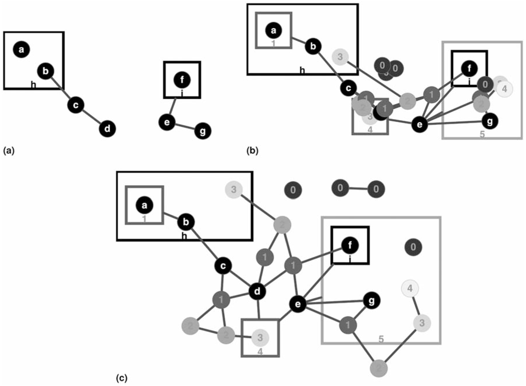
(a) A sample compound graph. (b) New nodes/edges are introduced by unhiding, where the nodes (the higher the rank, the lighter the fill color is) are placed using our algorithm in Algorithm 9, (c) followed by an incremental layout that tidies up the drawing, where the relative positions of original nodes (labeled a through i) are nicely kept while introducing the new content in a way respecting general graph drawing criteria.

Implementation & evaluation

As stated earlier, CMGV stands as an independent platform tailored for the management of graph complexity, featuring a cohesive model called CMGM. This model was meticulously implemented using JavaScript. Its primary design objective encompasses compatibility with diverse graph rendering libraries, facilitated through a dedicated CMGM API associated with the respective rendering framework. To exemplify its utility and evaluate its efficacy, we have adopted Cytoscape.js ⁹ as our rendering library of choice. Consequently, an interface has been implemented to establish seamless communication between the Cytoscape.js rendering engine and the CMGM. For an exhaustive exposition on the architecture and operation of this interface, refer to the Supplemental Material.

Experiment setup and dataset

Furthermore, we have designed and implemented a demo and test environment using our Cytoscape.js implementation of the framework. Test scripts implemented in this environment aim to test for the integrity of the framework as well as the measurement of various performance metrics using some test scenarios (see the Supplementary for details). A Supplemental Material video showing our framework in action, through a number of scenarios, using this demo, is also available.

These scenarios were executed on an ordinary computing platform (featuring an Intel i7-11700 2.50GHz CPU and 16GB of RAM) across a suite of randomly generated compound graphs. These compound graphs varied in size, spanning from 188 to 1032 nodes, and were sourced from the compound graph dataset established by Balci et al. ¹⁷ As detailed in their paper, they based this compound graph dataset on a subset of 81 graphs randomly chosen from the Rome dataset ⁴⁴ with a density not exceeding 3. In our study, we included denser graphs up to density 4.5 as well (Figure 12 of the Supplemental Material). To further refine the dataset, the Markov Clustering Algorithm ⁴⁵ was employed to identify clusters within each graph. Subsequently, nodes residing within each identified cluster were consolidated into a solitary compound node. This process was reiterated multiple times, leading to the generation of compound graphs with variable depths. Further information on properties of the experiment data and the scenarios used may be found in the Supplementary under Performance Evaluation.

Experiment results

Integrity tests performed on test graphs using the predetermined test scenarios were all completed successfully, leaving the topology of each compound graph intact.

We also measured the performance of the complexity management operations in terms of running time using two predefined scenarios on the test graphs. Scenario 1 includes a mixture of the three kinds of complexity management operations, while Scenario 2 also includes adding a random neighborhood to a randomly chosen node and repeating the test. Furthermore, we have a third scenario, which is randomly generated by selecting a do operation (e.g., collapse) before its undo (e.g., expand), where all kinds of operations are randomly determined and mixed (see the Supplemental Material for details). By varying the structure across these three scenarios, we aimed to simulate an arbitrary ordering of complexity management operations on graphs with randomized topology. Results are in line with our theoretical findings of the asymptotic linear run times of these operations (Figure 7).

Figure 7.

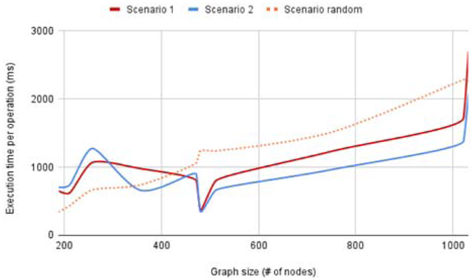
Graph size versus execution time for two predefined and one randomly generated scenario; results comply with asymptotic theoretical results of linear growth.

Furthermore, we investigated how complexity management operations and our customized layout affect the quality of the drawings. As can be seen in Figure 8 (and Figure 12 of the Supplemental Material for denser graphs), layout quality either improves or worsens marginally as complexity management operations are executed.

Figure 8.

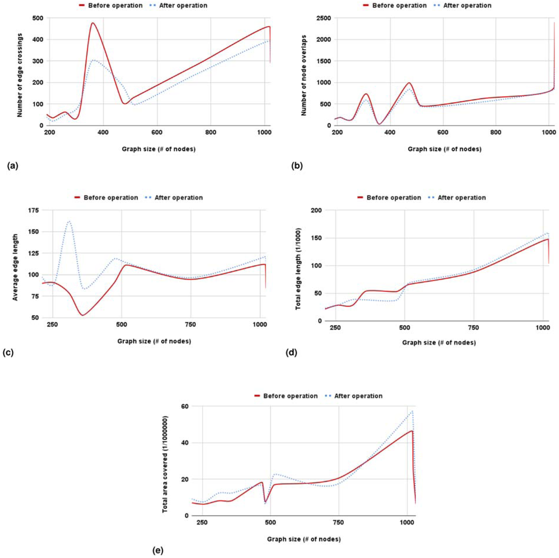
How various metrics of layout quality are affected by complexity management operations. The quality of the drawings across these five metrics remains largely consistent, with only occasional slight improvements or degradations. The results for node overlaps, total edge length, and total area are nearly identical. The observed reduction in edge crossings is likely due to the repeated incremental layouts triggered by each complexity management operation, which enhances layout quality in this aspect. The initial increase in average edge length can likely be attributed to expand/collapse operations, which introduce and remove inter-graph edges that tend to span longer distances. However, this effect is mitigated over time as successive incremental layouts are applied.

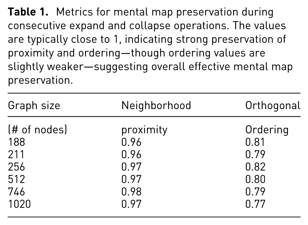
Finally, we also measured how the user’s mental map is preserved as these complexity management operations take place. Results show that neighborhood proximity is maintained almost fully, whereas orthogonal ordering is compromised slightly as taking out the unnecessary space around a collapsed node and introducing the space back on expand will inevitably disturb such ordering (Table 1).

Table 1.

Metrics for mental map preservation during consecutive expand and collapse operations. The values are typically close to 1, indicating strong preservation of proximity and ordering—though ordering values are slightly weaker—suggesting overall effective mental map preservation.

Graph size	Neighborhood	Orthogonal
(# of nodes)	proximity	Ordering
188	0.96	0.81
211	0.96	0.79
256	0.97	0.82
512	0.97	0.80
746	0.98	0.79
1020	0.97	0.77

To further evaluate the preservation of the mental map, we conducted a user study involving 24 participants with varying levels of expertise in graph visualization tools, including students, researchers, and software developers. Users were asked to perform a predefined set of operations and their corresponding undo actions in an order of their choice. They were then asked to comment on the difficulty of completing these tasks and whether they were able to maintain their mental maps throughout. The complete list of questions, along with participant profiles, is provided in the Supplemental Material under the User Study section.

As the results indicate (Figures 13–15 of the Supplemental Material), the framework was found to be easy to use, and users were able to keep track of the objects of interest as operations were carried out, giving an overall rating of 8.71 out of 10. Answers to specific questions include:

• Only three participants reported occasionally encountering errors or illegal states; however, follow-up indicated that these reports were due to misunderstandings—such as mistaking a suboptimal layout for an error—or a failure to carefully read the instructions. As a result, no genuine errors or illegal states were present.

• Again, only three participants responded “Occasionally” to the question regarding whether they felt lost or disoriented during the operations, while 12 responded “Never” and 9 responded “Rarely.”

As there are no existing frameworks or modules that can handle a similar set of operations in a mixed order, which is the very main motivation for our work, we were not able to make a comparison of results. Similarly, no existing specialized layout algorithm, such as fisheye lenses, can be used or would be rather inefficient for compound graphs with arbitrary levels of nesting.

Conclusion

Through manipulations on randomly generated graphs, we demonstrate the newly introduced framework CMGV’s proficiency in executing successive graph complexity management operations while upholding the integrity of the underlying data and maintaining the mental map of the user via customised layout algorithms. Another notable attribute is that the framework functions independently of rendering libraries and seamlessly integrates with various graph rendering libraries. This adaptability empowers CMGV to cater to diverse visualization needs, establishing its relevance across various domains.

In terms of future avenues, there is potential to introduce supplementary complexity management and analysis procedures. For instance, the incorporation of semantic zooming, wherein expansion and contraction of compound nodes occur in tandem with incremental and decremental graph zoom levels, is managed by the framework. Similarly, the novel layout algorithm introduced in this study primarily focuses on the expansion operation, but there are exciting prospects for further developments. This could encompass the integration of other complexity management operations involving the addition of graph elements, such as showing or unfiltering elements. Identifying the initial positions for unfiltered elements becomes crucial. These positions could be proximate to visible nodes linked to unfiltered graph nodes or aligned with their previous placement prior to the filtration process. Subsequently, the existing algorithm can expand the graph around these positions to assimilate the unfiltered elements. The current algorithm’s triumph in safeguarding the user’s cognitive map during the expansion operation serves as a solid foundation for subsequent investigations and advancements.

An implementation of our framework and methods is available on GitHub (https://github.com/ivis-at-bilkent/cmgm). An example usage of our framework is also implemented with the Cytsocape.js rendering library as a separate GitHub repository (https://github.com/ivis-at-bilkent/cytoscape.js-complexity-management). In this repository, a demo and a test application are also available for integrity and performance tests of our framework. All scenario and test graph-related files can also be found in a test directory of this repository.

Supplemental Material

sj-pdf-1-ivi-10.1177_14738716251383173 – Supplemental material for CMGV: Algorithms and a unified framework for complexity management in graph visualization

Supplemental material, sj-pdf-1-ivi-10.1177_14738716251383173 for CMGV: Algorithms and a unified framework for complexity management in graph visualization by Osama Zafar, Ugur Dogrusoz, Hasan Balci and Ahmet Feyzi Halac in Information Visualization