Sage Journals: Discover world-class research

Abstract

The increasing size of Big Data is often heralded but how data are transformed and represented is also profoundly important to knowledge discovery, and this is exemplified in Big Graph analytics. Much attention has been placed on the scale of the input graph but the product of a graph algorithm can be many times larger than the input. This is true for many graph problems, such as listing all triangles in a graph. Enabling scalable graph exploration for Big Graphs requires new approaches to algorithms, architectures, and visual analytics. A brief tutorial is given to aid the argument for thoughtful representation of data in the context of graph analysis. Then a new algebraic method to reduce the arithmetic operations in counting and listing triangles in graphs is introduced. Additionally, a scalable triangle listing algorithm in the MapReduce model will be presented followed by a description of the experiments with that algorithm that led to the current largest and fastest triangle listing benchmarks to date. Finally, a method for identifying triangles in new visual graph exploration technologies is proposed.

Keywords

Graph scalable algorithms triangle counting visual analytics parallel programming MapReduce

Introduction

Data, data, data, and more data! Obtaining data is just the beginning of analysis, but heaping piles of raw data are rarely useful. How data are structured or represented facilitates analysis. Data must undergo transformation, translation, transmuting and other structuring, categorization, and organization operations to enable intelligent analysis. This includes making data more concise, more relevant, and structured to improve the performance of a query or algorithm. Ultimately, data form the raw material we need to pave the roads to knowledge, and visualization is the interface to insight. The entanglement between data representation and analysis is best exemplified in the graph-theoretic study of complex networks.

With the era of Big Data¹ comes the emergence of Big Graphs,² and while there has been attention to improving the capacity of graph primitives, such as Breadth-First Search,^3,4 it should not be overlooked that the answers to even simple questions, the algorithm output itself, can be tremendously large and complex. Consider the task of identifying all mutually connected triplets in a graph or network of entities, often depicted as a triangle where each vertex of the triangle represents an entity that is connected to the other entities by the edges of the triangle. Finding all such triangles in a graph requires a lot of computation and the number of triangles can be many times more than the number of entities. Despite a triangle being a simple graphic, visualizing all triangles in a graph is very difficult because the triangles overlap and are easily obscured.

Computing triangles in graphs is a fundamental operation in graph theory and has wide application in the analysis of social networks,⁵ identifying dense subgraphs⁶ and network motifs,⁷ spam detection,⁸ and uncovering hidden thematic layers in the World Wide Web.⁹ Yet, given the attention to finding, counting, and enumerating triangles, there has been very little work done to present a visual representation of triangles that is both scalable and navigable. This may be due in part to the lack of feasible technology that can list out trillions of triangles to provide the specificity needed in a Big Graph visual analytic, where every triangle can be traced by an end-user.

This article will begin first with an exercise to convince the reader of the importance of not just more and bigger data, but also how the underlying representation of data can better enable knowledge discovery in the context of graph analytics. Then a new algebraic method to reduce the number of arithmetic operations for computing all triangles in a graph will be introduced, and additionally a new scalable algorithm that demonstrates the largest triangle enumeration to date will be presented, along with the experimental results. Finally, a method for extending existing algorithms in visual graph exploration tools to include the identification of triangles will be proposed.

An illustration of knowledge manifestation

Consider a network of things, where each thing is identified by a number and these things self-organize into a larger network of a Thing of Things. How do we represent this Thing of Things?

Tabulating

A set of binary relationships, e.g. one thing is associated with another thing, can be simply tabulated in a basic data structure, a list of pairs of things, that is compact and does not require any special management. This is illustrated by the subset of our network of Thing of Things shown in Figures 1(a) and 1(b). Note how 498 connects to 5 and 33—does this suggest a mutual relationship? Does the fact that 17 connects to 7, which connects 33 and in turn connects back to 17 denote transitive closure?

Figure 1.

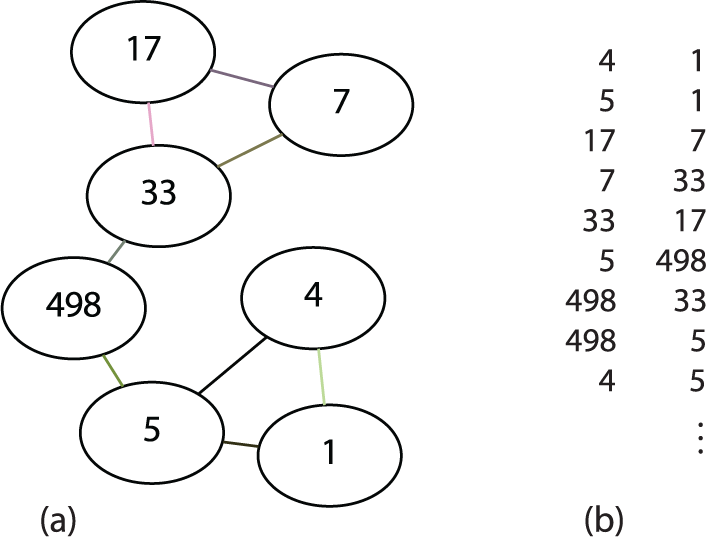
Thing of Things. (a) Sub-network. (b) List of binary relationships.

That’s just a tiny sample. Our Thing of Things comprises 500 things, which participate in 25,936 relationships. What can you identify, given all of the data as depicted in Figure 2? Displaying this very small example dataset provides very little insight. Tabulation can obscure non-direct relationships. Will a graph layout manifest information better? Complex relationships naturally form networks, which are ideal for graph treatment, so let’s Graph it!

Figure 2.

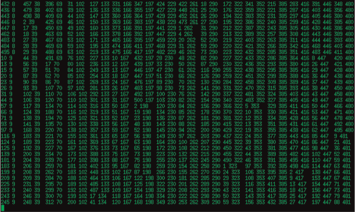
The full Thing.

Graphing

A graph can be displayed in a node–link layout, which appears as the familiar “ball and springs” model. But layout algorithms for graph visualization can have dramatic differences. Using the Graphviz graph visualization package available at www.graphviz.org, to produce Figure 3 our Thing of Things appears more like a ball of yarn with the “force-directed” layout. This doesn’t uncover any more useful information, colorful or not, than the tabulation example in Figure 2. But when the “scalexy” layout is used, as shown in Figure 4, there is a clearly emerging structure! By a simple change in displaying the graph data, three well-defined clusters can be identified in our Thing of Things network. Other visualization approaches can manifest these clusters in more striking fashion, but require another change in the graph representation.

Figure 3.

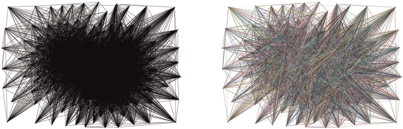
Graphviz “force-directed” layout.

Figure 4.

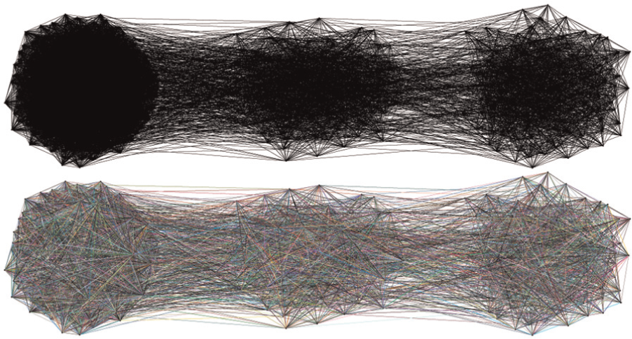
Graphviz “scalexy” layout.

Graph data structures

The following terms and definitions will be used throughout this article. Let $G = (V, E)$ denote a simple, undirected graph with $n = | V |$ vertices and $m = | E |$ edges, where $N (v) = {u \in V | (v, u) \in E}$ is the neighborhood of a vertex v, $d (v) = | N (v) |$ is its degree, and $d_{max} = max {d (v) | v \in V}$ is the maximum degree in G. Then $A \in ℝ^{n \times n}$ is the adjacency matrix of G, and so $A^{T} = A$ .

A graph data structure can be a list of pairs, e.g. edges, as noted earlier. In this edge-list representation, there are 2m ordered pairs including permutation, e.g. $(1, 2)$ and $(2, 1)$ , requiring 4m words of storage for all vertices, which is the minimum space needed for a complete representation of the graph dataset. Another graph data structure is the adjacency matrix, where the graph is represented in matrix form instead of as a list of edges. Each row represents an adjacency, i.e. neighborhood, of a vertex. Every non-zero entry indicates an edge, thus $A (i, j) = 1$ identifies an edge between vertices i and j. Recall that in matrix algebra zero is an annihilator for multiplication, so it is more efficient to use a sparse matrix representation for sparse graphs that ignores zero entries. Conventionally, G is sparse if $m \in O (n)$ . Using a dense matrix for G requires $O (n^{2})$ space. In contrast, storing G in a sparse matrix form requires $n + 4 m \in O (n + m)$ space, assuming the graph is connected. For a concrete example, consider the Yahoo! Web Graph derived from the Altavista search engine crawl of the World Wide Web circa 2002, available from Yahoo! at www.yahoo.com (https://webscope.sandbox.yahoo.com). This graph consists of $n = 1.4 \times 10^{9}$ web pages and $m = 6.6 \times 10^{9}$ URL links. To store this graph in matrix form would require space of the order of order of

gigabytes = {\begin{matrix} 230, 000, 000 & dense matrix \\ 3.2 & sparse matrix \end{matrix}

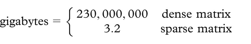
The dense matrix storage for this graph is prohibitive at nearly 230 petabytes whereas in contrast the sparse matrix is over seven orders of magnitude smaller, at just 3.2 gigabytes. A sparse matrix can be plotted and visualized in MATLAB, which can reveal patterns in the distribution of non-zero entries, so let’s Spy it!

Plotting

The Thing of Things edge list can be converted into a sparse matrix and visualized as a Spy plot in MATLAB. First annotate each edge with a 1 for the MATLAB conversion, then use the following commands:

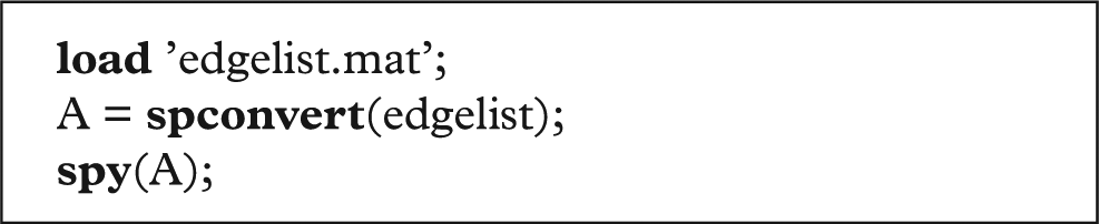
The Spy plot from this labor is provided in Figure 5. If the reader squints carefully, a pattern, albeit fuzzy, might be apparent, especially along the diagonal, but there is nothing definite enough to justify a purchase in new eyeglasses! However, is it possible to manipulate the graph matrix to reveal the clusters that were manifested in Figure 4?

Figure 5.

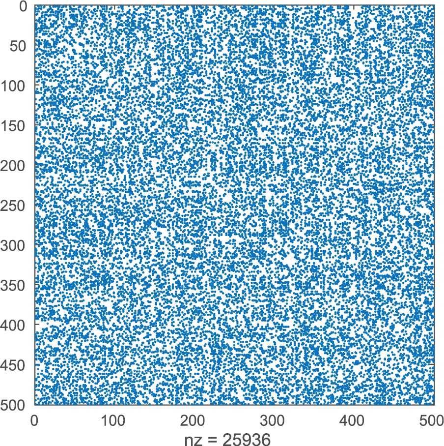
MATLAB Spy Plot.

Spectral partitioning

Let’s try spectral partitioning but this requires another change in representation of the data, specifically a new graph matrix, known as the graph Laplacian. The eigenvectors of this Laplacian can be used to partition the graph. The following definitions will be used in the next passages on spectral partitioning.

D diagonal matrix with vertex degrees along the diagonal;

L graph Laplacian, $L = D - A$ ;

U matrix whose columns are the eigenvectors of L.

The graph Laplacian is also symmetric and positive semi-definite, so the eigenvalues of L must be greater than or equal to zero. The multiplicity of the zero eigenvalue relates to the number of connected components in the graph. The eigenvector of the second smallest eigenvalue of L is the Fiedler eigenvector, whose namesake discovered its connection to graph connectivity and use in spectral partitioning.¹⁰ Reordering the adjacency matrix A by the sorted elements in the Fiedler eigenvector helps in envelope reduction to avoid fill-in, increases in non-zeros, during sparse matrix computations,¹¹ and also to reveal small-world characteristics in graphs.^12,13 This reordering technique will be helpful in visualizing clusters in the Thing of Things network. The premise in the reordering of A by a permutation vector is to align the non-zero entries close to the diagonal in A, thereby reducing the geometric distances between vertices, which results in natural partitioning of the graph. The following MATLAB commands will reorder A by the Fiedler eigenvector and Spy it!

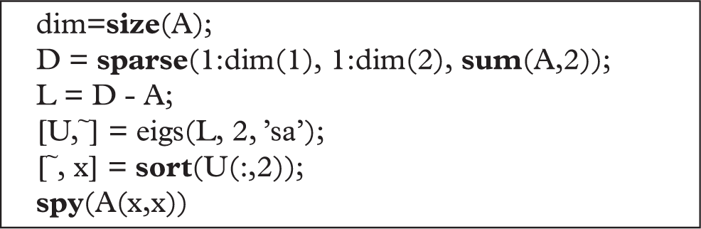
Behold, in Figure 6 three well-defined clusters are identifiable. Data representation matters! The choice of representation facilitates knowledge discovery. But it doesn’t end with just the original data. Data begets data. Data analysis output can be many times larger than the input!

Figure 6.

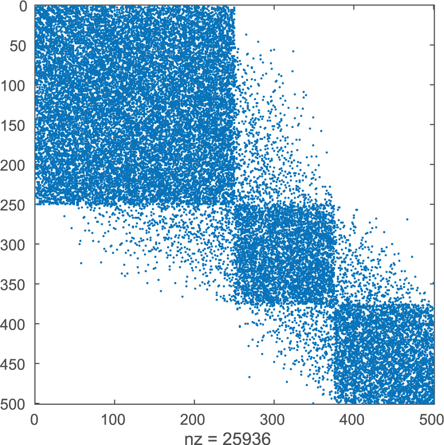
Spectral Partitioning.

Triangles in graphs

A triangle in G is a group of three vertices that are all mutually connected, thus it is a clique, i.e. a graph in which every vertex is connected to every other vertex, and a cycle, i.e. a path with identical endpoints. Triangles in graphs are useful for complex network analysis based solely on structural, i.e. adjacency, information. Let $Δ (v)$ be the local count of triangles involving vertex v and $Δ (G)$ be the global count of triangles in G. There can be many more triangles than vertices and edges, and if the graph is completely connected, where G itself is a clique, the total number of triangles, $Δ (G)$ , is

Δ (G) = (\begin{matrix} n \\ 3 \end{matrix}) \in Θ (n^{3})

The triangles in a graph can be easily identified by testing all possible triples, ${u, v, w}$ , for ${u, v}, {v, w}, {u, w} \in E$ , but this takes $O ((\begin{matrix} n \\ 3 \end{matrix})) \in O (n^{3})$ time. If most of the triples were triangles and the task was to enumerate all triangles, then the approach is optimal. But generally this brute force method is highly inefficient. We will briefly review the standard method for counting triangles leading to a new matrix approach, then transition into the description of a new algorithm that can potentially enumerate trillions of triangles.

Counting triangles

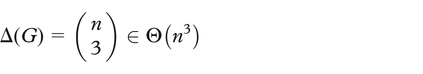
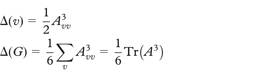
Since cycles of length n are diagonal elements in $A^{n}$ and a triangle is a cycle of length 3, then it is well known that the local and global triangle counts can be calculated by

\begin{matrix} Δ (v) = \frac{1}{2} A_{vv}^{3} \\ Δ (G) = \frac{1}{6} \sum_{v} A_{vv}^{3} = \frac{1}{6} Tr (A^{3}) \end{matrix}

where the symbol $Tr$ will refer to the trace operator of a matrix. The $\frac{1}{2}$ factor in $Δ (v)$ is to account for the cycles from ${u, w}$ incident to v, and the factor $\frac{1}{6} = \frac{1}{2} \times \frac{1}{3}$ in $Δ (G)$ is because each triangle is counted thrice.

Computing triangles by $A^{3}$ by fast matrix multiplication admits the best runtime of $n^{ω + o (1)}$ , where $ω ⩽ 2.3728639$ is the fast matrix product exponent.¹⁴ But the classic matrix product is used in practice, therefore practical improvements would be beneficial. A new matrix approach developed in 2013 by this author reduces the total number of arithmetic operations.¹⁵ Here the element-wise multiplication operator for matrices is denoted by the $\circ operator$ .

Theorem 1. Given G and the Hadamard product $(A^{2} \circ A)$ , then $Δ (v) = \frac{1}{2} \sum_{v} A^{2} \circ A {(A^{2} \circ A)}_{v}$ and $Δ (G) = \frac{1}{6} \sum_{i j} {(A^{2} \circ A)}_{i j}$ .

Proof. The paths of length two, i.e. 2-paths, are identified by $A^{2}$ ; then element-wise multiplication $A^{2} \circ A$ retains only those ${v, u}$ endpoints of 2-paths that are also the ${v, u} \in E$ endpoints of edges. Then the sum of elements in the v^th column vector of $A^{2} \circ A$ is the number of 3-cycles involving v. Using $Δ (v) = \frac{1}{2} A_{vv}^{3}$ leads to

Δ (v) = \frac{1}{2} A_{v v}^{3} = \frac{1}{2} \sum_{v} {(A^{2} \circ A)}_{v}

(1)

Now recall $Tr (X Y^{T}) = \sum_{i j} {(X \circ Y)}_{i j}$ ; then $Tr (A^{2} A^{T}) = \sum_{i j} {(A^{2} \circ A)}_{i j}$ . Finally, since $Δ (G) = \frac{1}{6} Tr (A^{3})$ , then

Δ (G) = \frac{1}{6} Tr (A^{3}) = \frac{1}{6} Tr (A^{2} A^{T}) = \frac{1}{6} \sum_{i j} {(A^{2} \circ A)}_{i j}

(2)

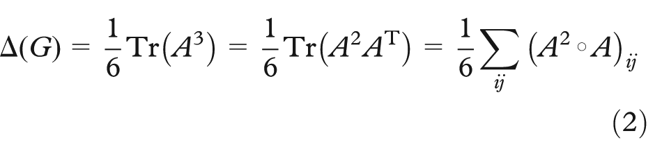
The corollary to this is that the number of arithmetic operations is cut in half when using classic matrix multiplication.

Corollary 1. The number of arithmetic operations for counting all triangles in G by Theorem 1 using sparse matrix representation is $2 N (n + 1) - 1 = O (mn)$ , where $N = 2 m$ is the number of non-zeros, which is approximately half the number of arithmetic operations if counting by $Tr (A^{3})$ using sparse matrix products.

Proof. There are a total of $2 N$ multiplication and addition operations for a sparse matrix–vector product. Then $A^{2}$ is possible by direct application of sparse matrix–vector multiplication of A with all n column vectors in A for a total of $2 Nn$ arithmetic operations. Then $A^{2} \circ A$ takes N operations for the element-wise multiplication and, finally, summing all non-zero elements from this is an additional $(N - 1)$ operations. Thus, $\sum_{i j} {(A^{2} \circ A)}_{i j}$ requires $2 N (n + 1) - 1 = O (mn)$ arithmetic operations, since $N = 2 m$ . In contrast, computing $A^{3}$ takes $4 Nn$ operations and $Tr (A^{3})$ adds an extra $(N - 1)$ operations totaling $4 Nn + N - 1$ , which is of the order of twice the number of arithmetic operations, as

\frac{2 Nn + 2 N - 1}{4 Nn + N - 1} \approx \frac{2 Nn}{4 Nn} = \frac{1}{2}

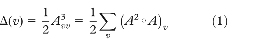
Using similar logic, it is easy to see that this result also holds for dense graphs and the local triangle count, $Δ (v)$ .

Computing triangles by Theorem 1 replaces a matrix multiplication requiring $O (n^{3})$ operations with a less expensive element-wise multiplication that requires only $O (n^{2})$ operations. Moreover, the new approach avoids a potential dense matrix multiplication, which can degrade the efficiency of sparse matrix multiplication. Although triangles can be enumerated by identifying common non-zero entries between $\vec{u}$ and $\vec{v}$ in $A^{2} \circ A$ for any {u, v} edge, the next section will describe a new algorithm that is better suited for enumerating trillions of triangles.

Scalable triangle listing

Disk-based computation for Big Data problems was popularized by the Google MapReduce paradigm¹⁶ and corresponding open-source Apache Hadoop framework (http://hadoop.apache.org). The theoretical model for MapReduce has been investigated,^17–19 putting it in firm standing with older computational models, such as Parallel Random Access Machine (PRAM), Bulk Synchronous Parallel (BSP), and Streaming. The largest Breadth-First Search on a graph was accomplished using the Hadoop MapReduce framework.⁴ The MapReduce model was also successful for the largest and fastest computation of all Jaccard similarity coefficients in a graph²⁰ at that time. The following sections will describe the MapReduce algorithm used in the largest and fastest enumeration of triangles in a graph to date.

MapReduce triangle listing algorithm

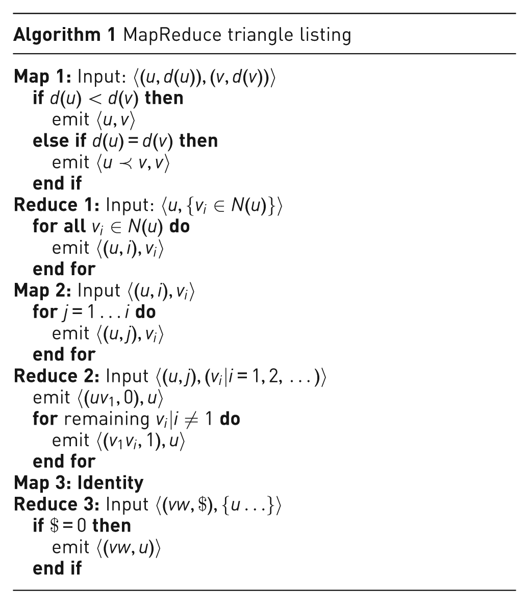
There are relatively few triangle algorithms in the MapReduce framework and these tend to focus on approximating triangles.^21,22 The most closely related work is that of Suri and Vassilvitskii²³ but that approach does not guarantee a constant amount of working memory needed for massively scalable algorithms. Moreover, the algorithm described here requires half the I/O by not revisiting the original graph edges; rather it uses the edges filtered by degree for subsequent triangle verification. The following is an outline for a new MapReduce triangle listing algorithm:

Filter out half the edges so that the end vertex has higher degree

(use lexicographic order, in case the degrees are equal).

Create labeled, ordered pairs by lexicographic order from the filtered edges:

Adjacent vertex pairs, i.e. endpoints of edges, labeled as edge;

Unique neighbor pairs, i.e. endpoints of 2-paths, labeled as non-edge;

List 2-paths for an ordered pair if it also has a label for an edge.

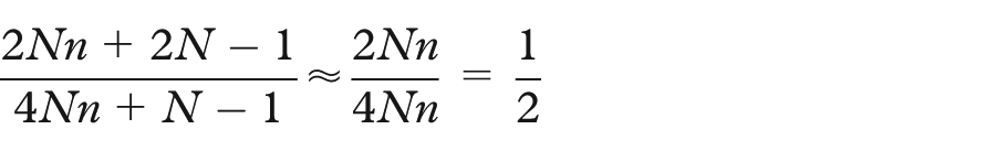
Like other algorithms,²⁴ the 2-paths are emitted only from the lowest-degree vertex in a triangle. This is enabled by the first step, which reduces the neighborhood of each vertex to contain only neighbors with higher degree. Denoting the size of this reduced neighborhood $d [v]$ , the work per vertex is $(\begin{matrix} d [v] \\ 2 \end{matrix})$ . Now observe that if a vertex has $\sqrt{m}$ neighbors, each with degree greater than $\sqrt{m}$ , it would exceed the number of edges in the graph. Thus, a vertex can only have $O (\sqrt{m})$ neighbors with higher degree. Subsequently, the work per vertex is $(\begin{matrix} d [v] \\ 2 \end{matrix}) ⩽ (\begin{matrix} \sqrt{m} \\ 2 \end{matrix}) = O (m)$ . It then follows that there is $O (\frac{m}{\sqrt{m}}) = O (\sqrt{m})$ work per edge, leading to an overall time-complexity of $O (m \sqrt{m}) = O (m^{3 / 2})$ , which is optimal for sparse graphs, since there could be $(\begin{matrix} \sqrt{m} \\ 3 \end{matrix}) = Θ (m^{3 / 2})$ triangles.

Although $d [v]$ can be quite large in highly skewed massive graphs, it is likely to be much less than $\sqrt{m}$ . Moreover, the $O (m)$ work to construct all neighbor pairs for a vertex can be load-balanced across parallel tasks, so for sparse graphs the algorithm will be scalable. The next section describes how to distribute the $(\begin{matrix} d [v] \\ 2 \end{matrix})$ neighbor pair construction in $O (1)$ words of working memory.

Load balancing

Unique pairs from a list of elements can be constructed in parallel while ensuring that each task performs a linear amount of work with constant words of memory, which are important for scalability. Consider the straightforward method, where the first element in the list is paired with the remaining $n - 1$ elements, then the second element is paired with the remaining $n - 2$ elements, and so forth. Now this can be accomplished in parallel by first constructing $n - 1$ lists, each containing one element fewer than the previous, and distributing these lists to multiple tasks. Then each task pairs the first element of its list with the remaining elements, simultaneously with all other tasks. The tasks require no more memory than needed to store a pair of elements, since each new element after the first replaces the previous element. It is also easy to generate these lists in $O (1)$ words of working memory by replicating each element by its ordinal in the original list.

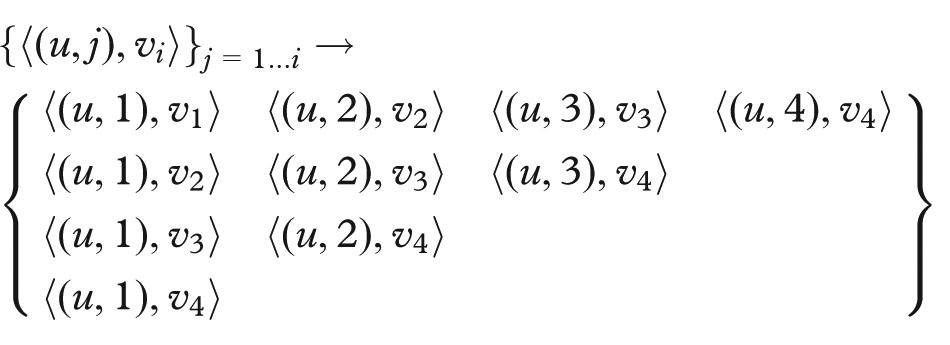
Now to construct all the unique neighbor pairs for a vertex u, each $v_{i} \in N (u)$ will be replicated by its i^th order in $N (u)$ , which is arbitrary but must be consistent. Then pairing u with each copy of $v_{i}$ is simply a matter of copying $v_{i}$ from $1 \dots i$ times, which requires only the memory needed to store $u, v$ . To distribute the $v_{i}$ copies with u for parallel, pairwise combination, a set of new $(u, j)$ compound keys is created. The new set of key-value pairs for a single vertex u and its neighbors in $N (u)$ is

{〈 (u, j), v_{i} 〉}_{j = 1 \dots i} \to {〈 (u, 1), v_{1} 〉 〈 (u, 2), v_{2} 〉 〈 (u, 3), v_{3} 〉 〈 (u, 4), v_{4} 〉 〈 (u, 1), v_{2} 〉 〈 (u, 2), v_{3} 〉 〈 (u, 3), v_{4} 〉 〈 (u, 1), v_{3} 〉 〈 (u, 2), v_{4} 〉 〈 (u, 1), v_{4} 〉}

Here the pairs are displayed in matrix layout only as a visual aid; in the computation, the pairs are distributed randomly by the MapReduce framework. Then, in a subsequent round, where values are aggregated and sorted for each $(u, i)$ key, the first value is paired with all remaining values. It is important that the values in each key are sorted to avoid duplicate pairing. The pairing is accomplished in $O (1)$ working memory, since only the first value is kept in memory and paired with the other values in a streaming fashion. The new Triangle Listing algorithm that takes $O (1)$ working memory and rounds is now given in Algorithm 1.

Algorithm 1 MapReduce triangle listing
Map 1: Input: $〈 (u, d (u)), (v, d (v)) 〉$
if $d (u) < d (v)$ then
emit $〈 u, v 〉$
else if $d (u) = d (v)$ then
emit $〈 u ≺ v, v 〉$
end if
Reduce 1: Input: $〈 u, {v_{i} \in N (u)} 〉$
for all $v_{i} \in N (u)$ do
emit $〈 (u, i), v_{i} 〉$
end for
Map 2: Input $〈 (u, i), v_{i} 〉$
for $j = 1 \dots i$ do
emit $〈 (u, j), v_{i} 〉$
end for
Reduce 2: Input $〈 (u, j), (v_{i} \| i = 1, 2, \dots) 〉$
emit $〈 (u v_{1}, 0), u 〉$
for remaining $v_{i} \| i \neq 1$ do
emit $〈 (v_{1} v_{i}, 1), u 〉$
end for
Map 3: Identity
Reduce 3: Input $〈 (vw, $), {u \dots} 〉$
if $$ = 0$ then
emit $〈 (vw, u) 〉$
end if

The $1 \dots i$ replication of each neighbor vertex in the first step, analogous to the generation of anti-diagonals in a circulant matrix, can also degrade performance when a single task must generate many copies for a large i value. It is simple to partition and distribute the replication work to other tasks, but this detail is left out for brevity. Also, this method generalizes to creating unique pairs in parallel from any set of elements using $O (1)$ words of working memory; this can be useful in streaming and other external-memory applications.

Triangle listing benchmarks

The new MapReduce triangle listing algorithm was demonstrated in a two-part experiment. The first part was to test the algorithm on real-world graphs that would be easily repeatable by other practitioners. The second part was a scalability test. The results of the experiment were first presented in the keynote address for the IEEE Exploring Graphs at Scale (EGAS) 2015 workshop.²⁵ The benchmarks were carried out on a cluster of 880 nodes with 24 cores and 64 GB RAM per node. The datasets were modified so that each edge was annotated by degree, e.g. $〈 (u, d (u)), (v, d (v)) 〉$ . An additional MapReduce job was inserted after the first round to randomize the output, resulting in a total of four rounds to list all triangles.

Part 1

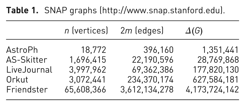
The datasets for this part of the experiment, listed in Table 1, were downloaded from the Stanford Network Analysis Project (SNAP, http://www.snap.stanford.edu). The graphs were undirected and the global triangle count was available for ground truth. The benchmark results are provided in Figure 7 and demonstrate that Algorithm 1 takes less than 5 min on average for these small graphs; this is still comparatively slow because of the overhead needed for parallel processing and reading from disk. The second part of the experiment is more compelling.

Table 1.

SNAP graphs (http://www.snap.stanford.edu).

	n (vertices)	2m (edges)	$Δ (G)$
AstroPh	18,772	396,160	1,351,441
AS-Skitter	1,696,415	22,190,596	28,769,868
LiveJournal	3,997,962	69,362,386	177,820,130
Orkut	3,072,441	234,370,174	627,584,181
Friendster	65,608,366	3,612,134,278	4,173,724,142

Figure 7.

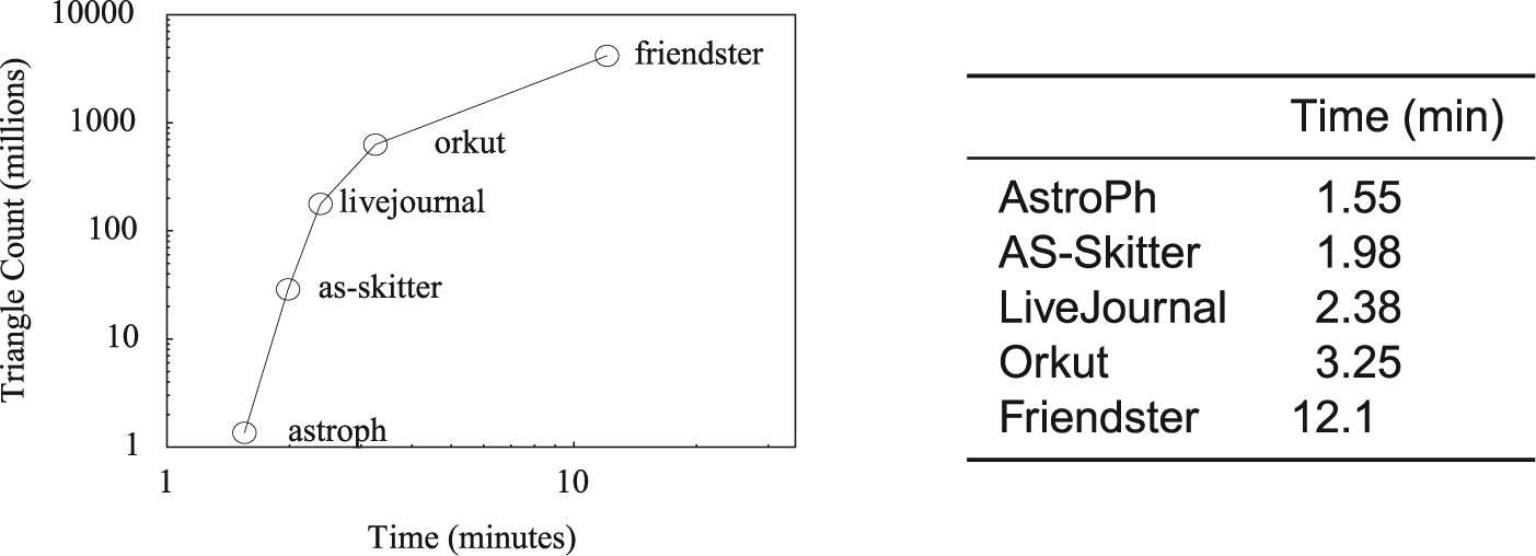
Triangle listing results for SNAP datasets.

Part 2

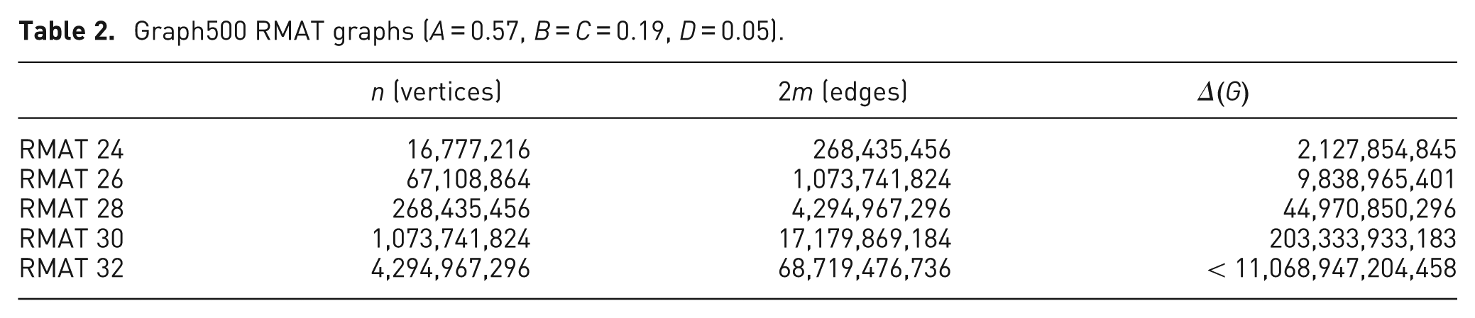
To test scalability, the Algorithm 1 was benchmarked on synthetically generated datasets using the Graph500 (www.graph500.org) benchmark parameters. Table 2 lists the sizes of the graphs and the triangle counts computed by the algorithm. The results of this benchmark are given in Figure 8. The top performance was listing 1.6 billion triangles per minute! This was achieved on the RMAT scale 30 graph with $Δ (G) > 200$ billion, which was 1.8 TB in size; to the best of this author’s knowledge it is the largest and fastest triangle listing experiment. The RMAT 28 and larger graphs have a maximum degree on the order of $10^{6}$ but because of the aforementioned load-balancing technique, the neighbor pairing for high-degree vertices was distributed across many reduce tasks, demonstrating the efficacy of the approach. Moreover, the number of 2-paths output from the RMAT 30 graph was nearly two trillion and for the RMAT 32 graph exceeded eleven trillion. The experiment on the RMAT 32 graph did not complete owing to time constraints and not failure.

Table 2.

Graph500 RMAT graphs ( $A = 0.57$ , $B = C = 0.19$ , $D = 0.05$ ).

	n (vertices)	2m (edges)	$Δ (G)$
RMAT 24	16,777,216	268,435,456	2,127,854,845
RMAT 26	67,108,864	1,073,741,824	9,838,965,401
RMAT 28	268,435,456	4,294,967,296	44,970,850,296
RMAT 30	1,073,741,824	17,179,869,184	203,333,933,183
RMAT 32	4,294,967,296	68,719,476,736	<11,068,947,204,458

Figure 8.

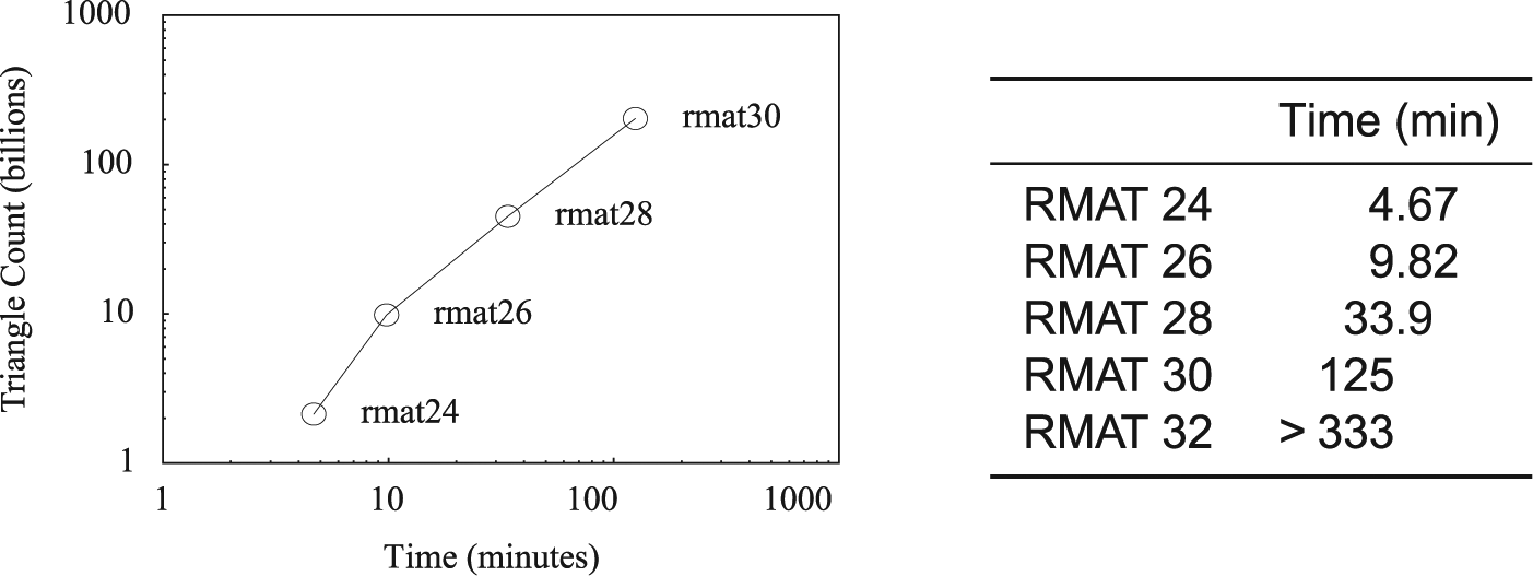
Triangle listing results for Graph500 datasets.

Visualizing trillions of triangles

Having established an algorithm capable of listing potentially trillions of triangles in a graph, the next step is to identify how to visualize the triangles. To begin, we need a scalable visual analytics platform but there are very few tools designed for large-scale graph exploration. The GreenHornet²⁶ visual analytics tool is designed for scalability and utilizes a hierarchical partitioning of the graph, exemplifying the importance of data representation. The data hierarchy in GreenHornet is a sequence of increasingly coarser partitions of the graph, generated by merging vertices of lowest degree to their neighbors. If this merging process also identified common neighbors of the merged vertices, it would identify triangles, performing what is widely-known as an edge iterator algorithm for counting or listing triangles where for every ${v, u}$ edge any $w \in N (v) \cap N (u)$ completes the ${v, u, w}$ triangle. Moreover, if any $u, w$ neighbors, to be merged into a vertex v, having degrees at most $\sqrt{m}$ , were instead tested for ${u, w} \in E$ , which is possible in $O (1)$ time, the runtime would be $O (m^{\frac{3}{2}})$ , which is optimal.²⁴

Recent development is now encroaching on trillion-edge scale graph exploration,²⁷ which could admit the navigation of trillions of triangles in a graph. The multiscale layout algorithm of Wong et al.²⁷ is reported to be similar to the merging algorithm in GreenHornet and could therefore be extended in the aforementioned merging proposal of neighboring vertices to identify triangles. This will pave the way forward to Big Graph exploration not only of the input graph but also of the overlay of the graph analytic products with the input.

Footnotes

Acknowledgements

The author thanks David G Harris and Louis W Ibarra for their helpful comments.

Funding

This research received no specific grant from any funding agency in the public, commercial, or not-for-profit sectors.

References

Burkhardt

. An overview of big data. The Next Wave 2014; 20(4): 4–10.

Burkhardt

. Big graphs. The Next Wave 2014; 20(4): 11–20.

Burkhardt

Waring

. An NSA big graph experiment. Technical Report NSA-RD-2013-056001v1, US National Security Agency, 2013.

Burkhardt

Waring

. A cloud-based approach to big graphs. In: Proceedings of the 19th annual IEEE conference on high performance extreme computing, Waltham, MA, 15–17 September 2015, pp.1–8. Piscataway, NJ: IEEE.

Watts

Strogatz

. Collective dynamics of ‘small-world’ networks. Nature 1998; 393(6684): 440–442.

Cohen

. Graph twiddling in a MapReduce world. Comput Sci Eng 2009; 11(4): 29–41.

Milo

Shen-Orr

Itzkovitz

. Network motifs: simple building blocks of complex networks. Science 2002; 298(5594): 824–827.

Becchetti

Boldi

Castillo

. Efficient algorithms for large-scale local triangle counting. ACM Trans Knowl Discovery Data 2010; 4: 1–28.

Eckmann

Moses

. Curvature of co-links uncovers hidden thematic layers in the World Wide Web. Proc Natl Acad Sci USA 2002; 99: 5825–5829.

10.

Fiedler

. Algebraic connectivity of graphs. Czech Math J 1973; 23: 298–305.

11.

Barnard

Pothen

Simon

. A spectral algorithm for envelope reduction of sparse matrices. In: Proceedings of the 1993 ACM/IEEE Conference on Supercomputing, Portland, OR, 15–19 November 1993, pp.493–502. Piscataway, NJ: IEEE.

12.

Grindrod

. Range-dependent random graphs and their application to modeling large small-world proteome datasets. Phys Rev E 2002; 66: 066702-1–066702-7.

13.

Higham

. Unravelling small world networks. J Comput Appl Math 2003; 158: 61–74.

14.

Le Gall

. Powers of tensors and fast matrix multiplication. In: Proceedings of the 39th International Symposium on Symbolic and Algebraic Computation, Kobe, Japan, 23 July 2014, pp.296–303. New York, NY: ACM.

15.

Burkhardt

. Internal NSA conference presentation, 2013.

16.

Dean

Ghemawat

. MapReduce: simplified data processing on large clusters. In: Proceedings of the 6th conference on symposium on operating systems design and implementation, San Francisco, CA, 2004, pp.137–150. Berkeley, CA: USENIX Association.

17.

Karloff

Suri

Vassilvitskii

. A model of computation for MapReduce. In: Proceedings of the 21st annual ACM-SIAM symposium on discrete algorithms, Austin, TX, 2010, pp.938–948. Philadelphia, PA, SIAM.

18.

Goodrich

Sitchinava

Zhang

. Sorting, searching, and simulation in the MapReduce framework. In: Asano

Nakano

Okamoto

. (eds) Algorithms and computation. Berlin: Springer, pp.374–383.

19.

Pietracaprina

Pucci

Riondato

. Space-round tradeoffs for MapReduce computations. In: Proceedings of the 26th ACM international conference on supercomputing, San Servolo Island, Venice, Italy, 2012, pp.235–244. New York, NY: ACM.

20.

Burkhardt

. Asking hard graph questions. Technical Report NSA-RD-2014-050001v1, US National Security Agency, 2014.

21.

Tsourakakis

Kang

Miller

. Doulion: counting triangles in massive graphswith a coin. In: Proceedings of the 15th ACM SIGKDD international conference on knowledge discovery and data mining, Paris, France, 2009, pp.837–846. New York, NY: ACM.

22.

Pagh

Tsourakakis

. Colorful triangle counting and a MapReduce implementation. Inf Process Letts 2012; 112: 277–281.

23.

Suri

Vassilvitskii

. Counting triangles and the curse of the last reducer. In: Proceedings of the 20th international conference on World Wide Web, Hyderabad, India, 28 March 2011, pp.607–614. New York, NY: ACM.

24.

Latapy

. Main-memory triangle computations for very large (sparse (power-law)) graphs. Theor Comput Sci 2008; 407: 458–473.

25.

Burkhardt

. Graph it! Vis it! Technical report, US National Security Agency, http://www.vacommunity.org/egas2015/papers/IEEEEGAS2015-PaulBurkhardt.pdf (accessed October 26, 2015).

26.

Wong

Mackey

Cook

. A multi-level middle-out cross-zooming approach for large graph analytics. In: Proceedings of the 2009 IEEE symposium on visual analytics science and technology, Atlantic City, NJ, 12–13 October 2009, pp.147–154. Piscataway, NJ: IEEE.

27.

Wong

Haglin

Gillen

. A visual analytics paradigm enabling trillion-edge graph exploration. In: Proceedings of the 2015 IEEE Symposium on Large Data Analysis and Visualization, Chicago, IL, 25–26 October 2015, pp.57–64. Piscataway, NJ, IEEE.

Graphing trillions of triangles

Abstract

Keywords

Introduction

An illustration of knowledge manifestation

Tabulating

Graphing

Graph data structures

Plotting

Spectral partitioning

Triangles in graphs

Counting triangles

Scalable triangle listing

MapReduce triangle listing algorithm

Load balancing

Triangle listing benchmarks

Part 1

Part 2

Visualizing trillions of triangles

Footnotes

Acknowledgements

Funding

References