
Abstract
Motivated by the analysis of chemical metal compounds and their properties for catalysis, we developed a gradient boosting model that explores graph structures to perform prediction tasks. Taking advantage of the iterative nature of boosting, our novel approach, called
Introduction
Understanding the relationship between the structure of a molecule and its properties is a cornerstone of numerous domains, such as medicinal chemistry (Dara et al., 2022) and materials science (Butler et al., 2018). These molecular structures embody graph-based information, where atoms are represented as nodes and the bonds as edges. Predicting molecular properties from these intricacies presents analytical challenges due to the data’s high dimensionality, non-linearity and inherent complexity.
The relationship between a molecular structure and a property of interest can be computed through complex quantum-mechanics computations (Balcells and Skjelstad, 2020), but the computations require many computer hours, resulting in an extremely time-consuming and environmentally unfriendly process. A different strategy consists of learning the relationships by exploiting a statistical learning approach, which is trained on existing data and used to predict unseen cases. Many approaches have been developed to this aim, including graph neural networks (GNNs, see, e.g. Jørgensen et al., 2018; Schütt et al., 2018; Kneiding et al., 2023) and boosting (e.g., Kudo et al., 2004; Saigo et al., 2009; Fei and Huan, 2010; Pan et al., 2017). The former (GNNs) provide very good results in terms of prediction and are therefore regarded as the state of the art. Nevertheless, they are black-boxes that do not allow to infer new information from the trained model (Scarselli et al., 2009). The inherent opacity of GNNs poses significant challenges to comprehending the mechanism regulating the property of interest, making their practical use particularly unattractive in chemistry applications (Wu et al., 2021).
In this article, we choose to follow a boosting strategy instead. Advantages of the proposed boosting procedure include variable selection, explainability (variable importance) and resistance towards overfitting. In contrast to the boosting approaches currently available in the literature to handle graph-structured input data, which first search for the optimal patterns and then apply a boosting algorithm (see, e.g., Kudo et al., 2004), we simultaneously perform the search for the relevant paths and the evaluation of their effects on the response. Our algorithm, indeed, updates the statistical learning model while exploring the graph. This is facilitated by the specific characteristics of the molecules we are investigating, namely the transition metal-organic compounds, which have a specific metal centre that we can use as the starting point for our search. The presence of distinct centres inspired us to explore parallelization during the training phase. We then devised an aggregation strategy that prioritizes genuinely relevant centres, rather than those that appear important merely due to the independent training performed on each centre. Our work is motivated by the analysis of the
The article is structured as follows: In Section 2 we describe our case of study and introduce the data; in Section 3 we describe the gradient boosting approach and our specific version for graph exploration and regression; the novel approach is illustrated and investigated through synthetic data in Section 4; and finally evaluated on the real data in Section 5. Section 6 concludes the article.
Motivating application
This work is motivated by the analysis of transition metal complexes. They make up a distinct category of chemical compounds that exhibit an extensive array of physical properties and consist of a metal centre, around which the molecular structure is developed. While transition metal complexes have been explored and utilized extensively in the past, more work is needed to fully understand their electronic properties. Knowing the latter, in particular, may lead to scientifically intriguing and practically beneficial discoveries (Khomskii, 2014), involving anti-diabetic compounds (Sodhi, 2019), bio-energy fuels (Yun, 2016) and electronic devices (Wang et al., 2012). In practice, in this study we use the data provided by Balcells and colleagues in their
The most relevant challenge in implementing a statistical learning algorithm in this context is arguably the data structure. As we mentioned in the introduction, the molecules are represented in the form of graphs, with the nodes representing the atoms and the edges the bonds. This means that the input information is not in the standard form of an n × p matrix. The 60 799 molecules have completely different sizes and the space of the possible paths is in practice too large for an exhaustive enumeration.
One important property of the molecular structure of the transition metal compounds that helps in our work is the presence of a uniquely identified metal centre. This property allows our algorithm to start the search for relevant structures from a specific point, the metal centre itself. The dataset contains compounds with 30 different metal centres, with different number of instances (see Figure S1 in the Supplementary Materials). Moreover, the relevant structures affecting the HOMO/LUMO gap of the molecule are not so far from the metal centre, supporting a sequential search that starts from the metal centre.
Here, the goal is to explore the molecular structure of the existing compounds and to use this information to predict the HOMO/LUMO gap of a new compound. The HOMO/LUMO gap is a continuous variable and we assume that its conditional distribution is Gaussian. Note that we aim to only use the topology of the molecular graph, without considering further information available for the nodes and the edges. This will be material for future work (see also Section 6).
PathBoost: Path-based boosting
In this section, we introduce PathBoost, as a scalable boosting algorithm for learning an additive regression model based on labelled paths. By transforming each graph into a vector of counts, where each count refers to a specific labelled path, the approach is able to deal with the issue of various-sized graphs, providing an interpretable representation of the original input graph. Moreover, the additive structure of the model maintains the interpretability of the transformed input in its predicted output. To enable efficient learning of the proposed model, we exploit the fundamentally iterative nature of boosting to sequentially build up the input space or the representation of the graphs, as part of the learning procedure.
Preliminaries and notation
At a general level, the considered problem is an instance of graph regression, where we want to predict a target response,
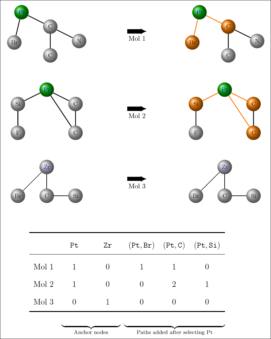
An illustration of how the feature matrix is expanded during training for a toy dataset containing three molecules. The first two feature columns represent the initial set of features Pt and Zr, as defined by the anchor node (i.e. the metal centre). After selecting Pt, all existing paths obtained by extending Pt by one node are (Pt,Br), (Pt,C), (Pt,Si) and these are added to the feature matrix and the corresponding feature values of each new path is the number of times the path occurs in the molecule.
An illustration of how the feature matrix is expanded during training for a toy dataset containing three molecules. The first two feature columns represent the initial set of features Pt and Zr, as defined by the anchor node (i.e. the metal centre). After selecting Pt, all existing paths obtained by extending Pt by one node are (Pt,Br), (Pt,C), (Pt,Si) and these are added to the feature matrix and the corresponding feature values of each new path is the number of times the path occurs in the molecule.
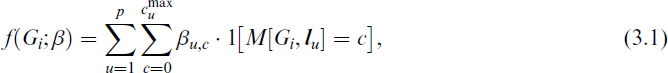
The graph regression problem amounts to learning a function

where u is the index or identifier of the labelled path. Moreover, we will use M[Gi,
Finally, and motivated by our application, we will assume that there is a single designated anchor node, denoted by v*, for each graph and we will focus on paths that start from this particular node. For a given set of training data,
The key challenge in graph regression, where the input graphs are of varying size, is to extract or construct features from the graphs that are informative for predicting the target response. By transforming each graph into a numerical vector of equal length,
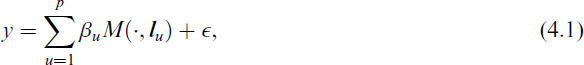
In this work we propose a hybrid feature learning approach where we define our feature space over all possible labelled paths, starting from the anchor node and define the associated features simply as the number of times the labelled path occurs in a graph. More specifically, using the above notation, each graph Gi will be mapped to a vector of counts with respect to a given collection of labelled paths, denoted by
where
In the assumed model class, the learning problem essentially consists of identifying the informative paths among all possible paths and fitting the path-specific coefficients,
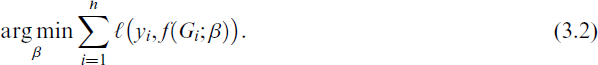
The above estimation problem is very challenging due to its high-dimensional nature. In practice, we assume that only a small fraction of the labelled paths are informative for predicting the target response and the key to efficient learning will rely on the ability to identify those paths as part of the learning procedure. To this end, we will employ boosting, which is a learning technique tailored to this type of setting.
More specifically, our algorithm is based on gradient boosting, which assumes a differentiable loss function and solves Equation (3.2) by iteratively approximating the negative gradient of the loss function with simple models, referred to as base learners. Then, to avoid overfitting, the algorithm is stopped at a certain iteration (mstop), which is typically estimated by cross-validation and the base learners are assembled into a final boosting model. In terms of the type of base learners, we focus on tree stumps which makes only a single split on a single variable. By using tree stumps we will avoid interactions between paths, which ultimately results in an additive model of the form in Equation (3.1). In addition, tree stumps have the property of being ‘weak’, meaning that one stump alone does not have too big of an improvement of the model, a property that has been proven to be fundamental for boosting (Bühlmann and Yu, 2003). For more information about the general technique of boosting, we refer the reader to the overview article by Mayr et al. (2014).
The main obstacle to a straightforward boosting procedure, as the one described above, is that the number of possible labelled paths quickly becomes too large for an exhaustive enumeration, even if we restrict the feature space to only the labelled paths observed in the given training set
We refer to the general algorithm that implements the above idea as
Path Importance
As a boosting algorithm,
PathBoost

PathBoost
The simplest way to define feature (or path) importance is to sum up the contribution of each selected path (that is, the one that leads to the largest reduction of the loss function) over all iterations. In the end, for each path, we will have a total reduction of the considered loss given by the inclusion of that path in the model. A different approach is to evaluate the difference in terms of the loss function not in absolute terms but relative to the second-best option. In this way, a path that could be substituted in the model by another path (with correlated feature values) and does not get an inflated importance, compared to almost equally important alternatives. On the other hand, the importance of two similarly informative paths may be underestimated, as they are interchangeable and a less relevant path is assigned a higher importance.
We will consider both of the above variants and we will rescale the path importance measure with respect to the most important path, such that final values range from 0 (no importance) to 100 (most important), as is standard in the statistical learning framework (Hastie et al., 2009, Ch. 10.13.1). In the adaptive setting, we note that only a small fraction of typically shorter paths are available for the algorithm to split on early in the learning phase, when most of the reduction in loss occurs. Thus, path importance measures based on loss reduction will implicitly favour shorter paths.
While the general method is fully described above, here we present the most relevant details of our particular implementation of
Simulations
Before applying our algorithm to the real data, we evaluate its behaviour in a controlled setting, that mimics the characteristics of the
Synthetic data
We generate synthetic data by following a simple procedure: We first identify some specific paths of the molecular structures that are present in a sufficiently large number (300) of compounds contained in the
where

and du is the length of the path. We added the latter term to simulate the chemists’ conjecture that the relevant structures are close to the metal centre.
We generate data in three different scenarios. Each scenario is run 200 times (replications), keeping the values of the regression coefficients fixed (they are generated only once). In every replication, the number of iterations, mstop, is computed via five-fold cross-validation and we set patience = 3.
Average true positive rate (TPR) as a function of the number of iterations. The shadowed area shows the range (interval between the smallest and highest value) of TPR in the 200 replications. Left panel: Scenario 1. Right panel: Scenario 2
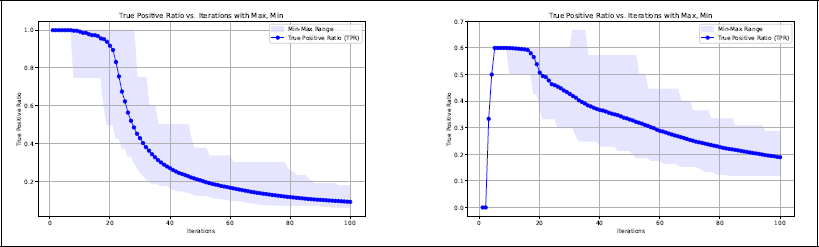
Scenario 1
As expected, the algorithm performs well in terms of variable selection in this highly simplified setting. The most complicated path,
Scenario 2
In this scenario, it is much more difficult for the algorithm to find the true paths. Although the relevant paths are nested in this case as well, they are farther from the metal centre and their effects are much smaller. Remember that the size of the coefficients β are inversely proportional to the path length (see Equation 4.2) and here we have one relevant path of length five. In addition, the algorithm necessarily needs to select some irrelevant paths, as the shortest relevant path
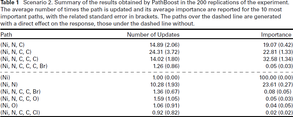
Scenario 2. Summary of the results obtained by PathBoost in the 200 replications of the experiment. The average number of times the path is updated and its average importance are reported for the 10 most important paths, with the related standard error in brackets. The paths over the dashed line are generated with a direct effect on the response, those under the dashed line without.
Scenario 2. Summary of the results obtained by PathBoost in the 200 replications of the experiment. The average number of times the path is updated and its average importance are reported for the 10 most important paths, with the related standard error in brackets. The paths over the dashed line are generated with a direct effect on the response, those under the dashed line without.
The above mentioned difficulties are reflected in the true positive rate (TPR), which is considerably lower than in the previous scenario, as shown in the right panel of Figure 2. From this figure, we can also see that in all 200 replications of the experiment the algorithm selects the noisy paths
After capturing the information of the relevant paths, the algorithm starts selecting noisy paths quite early, noticeably around the 17th iteration. The average stopping iteration mstop obtained by five-fold cross-validation in this scenario is 82.82 (SE = 20.85), meaning
Table 1 also shows the importance of the paths computed by
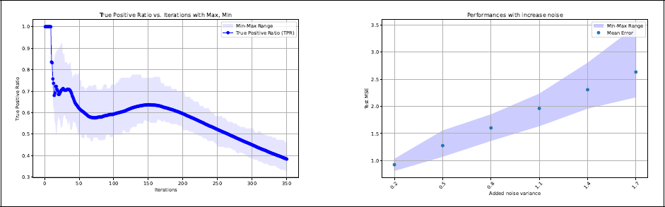
Scenario 3. Left panel: TPR as a function of the number of iterations. Right panel: Test error (mean squared error) as a function of the irreducible error. In both panels the shadowed area shows the interval between the smallest and the highest value (range) obtained in the 200 replications.
Finally, the error is relatively large, being on average 0.92 (SE = 0.19), compared to a generated irreducible error of σ2 = 0.2. This may again be partially explained by the selection of noisy paths close to the metal centre, in particular path
This is the most realistic scenario, with a higher level of difficulty for the algorithm to find the true generating model. This is reflected in a higher value of the stopping iteration obtained by the five-fold cross-validation procedure (average mstop = 312.32, with SE = 32.40). The increased number of iterations also led to an increase in the number of selected paths (on average 92.47, with SE = 10.83), including noisy ones (see left panel of Figure 3). As in Scenario 1,
We also evaluated the predictive performances of
Main application
We are now ready to apply
Implementation details
As is common in regression problems, here we use the squared error as the loss function. In terms of the boosting algorithm, we use tree stumps as base learners and a learning rate η = 0.3 to further ‘weaken’ them. The selected learning rate is the default value in many boosting implementations, including XGBoost (Chen and Guestrin, 2016).
Since gradient boosting is based on sequential improvements, it is usually not possible to parallelize the algorithm. In our case, however, each path grows from a specific anchor node or metal centre and paths that do not share the metal centre do not interact. In practice, this essentially means that our boosting algorithm fits a different sub-model for each specific class of compounds, where the class of compounds is defined by its metal centre. Importantly, this insight enables us to implement a form of parallelization that facilitates training on larger datasets. Specifically, we use the following computational trick: We first fit
Note that the above procedure is different from fitting 30 separate boosting models: By selecting the best update at each iteration, the algorithm potentially avoids updating paths that do not contribute to the general aim but are only useful for explaining a variation of a potentially irrelevant class of compounds, for example, all relevant information may already have been captured within that class. Moreover, it only requires the computation of a single mstop, that is, avoid performing 30 separate time-consuming cross-validation procedures.
To simplify the search for relevant paths, we also decided to limit the maximum path length to six. This is consistent with the conjecture that HOMO/LUMO gaps are mainly influenced by the characteristics of the molecules’ centres. Preliminary analyses (see Figure S3.2 in the Supplementary Materials) corroborated this idea. This simplification allows us to avoid long chains of carbon atoms, greatly speeding up the algorithm at a minimum cost (for more information, see Section 5.3).
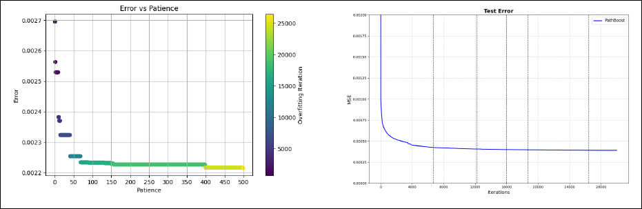
Regarding the tuning of the algorithm, the optimal number of iterations has been found by five-fold cross-validation, using a patience value equal to 68 following the elbow rule (this choice is discussed in Section 5.3, see also Figure 6). The mstop value obtained with this procedure is 15 948, resulting in a total of 64 186 considered paths, of which 9 700 were included in the final model.
Main application. Left panel: Test error as a function of the iterations. The vertical line shows the value of mstop obtained by five-fold cross-validation, the horizontal line the null model (only metal centres). Right panel: Scatter plot contrasting observed and predicted HOMO/LUMO gaps in the test set (at iteration mstop).
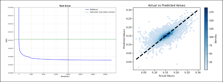
Main application. Left panel: Test error as a function of the iterations. The vertical line shows the value of mstop obtained by five-fold cross-validation, the horizontal line the null model (only metal centres). Right panel: Scatter plot contrasting observed and predicted HOMO/LUMO gaps in the test set (at iteration mstop).
Figure 4 summarizes the results of the case study. We obtained a test mean square error around 4 × 10⁻⁴, which is comparable to current competitors (see Section 5.3). Interestingly, from the left panel of Figure 4 we can also see that the test error continues to decrease after the stopping iteration has been reached. Therefore, in theory, our model would have profited from some additional iterations. However, the improvement after the selected iteration is limited and this early stop does not influence the quality of the prediction too much. Also note that, with very few exceptions, the predicted and the observed values of the HOMO/LUMO gap in the test set are in general reasonably similar (Figure 4, right panel).
As mentioned in Section 3, one relevant feature of
Main application. Top 30 paths by importance (left panel) and top 30 paths by importance when excluding the paths of length zero (right panel). Here the importance is defined as the sum of the overall improvements to the previous step and they are scaled in a way that the most important path has importance 100.
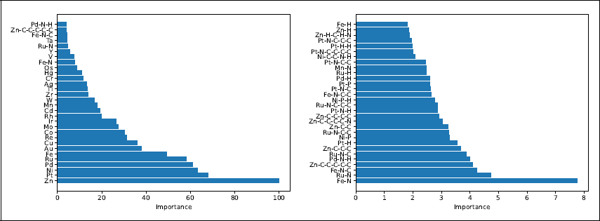
Main application. Top 30 paths by importance (left panel) and top 30 paths by importance when excluding the paths of length zero (right panel). Here the importance is defined as the sum of the overall improvements to the previous step and they are scaled in a way that the most important path has importance 100.
Main application. Left panel: Cross-validation error as a function of the patience. Right panel: Test error with the results of a few values of patience (namely 15, 41, 69, 157, 498) highlighted by vertical lines.
In addition to the main results, we can gain further insights into the algorithm’s performance by analysing the following points.
Conclusions
In this article, we proposed a boosting algorithm,
Concerning the target application, instead, it would be useful to increase the prediction ability of the model by incorporating the characteristics of the atoms and edges. Currently, our algorithm is only able to explore the molecular connectivity (graph topology), without considering quantities such as the atomic number of the atoms, the strength of the chemical bonds and so on. The inclusion of this additional information has been shown to be useful in the context of neural networks, where Kneiding et al. (2023) managed to reduce the error of a neural network by one order of magnitude. It seems very reasonable that the same will be true for a boosting algorithm and we are planning to extend
Considering the strength of a chemical bond in a boosting algorithm such as
One advantage of our algorithm is the ability to evaluate the variable importance. Our current implementation, based on the deviance, is simple and generally effective, but may face some difficulties in specific situations. For example, in the case of nested relevant paths, it is not guaranteed that the variable importance is correctly allocated among the paths (tendentially, shorter paths are favoured). Handling cases like this is not straightforward and the algorithm would benefit from future work on this issue.
Finally, one simplification directly connected to our chemistry application is the presence of a single anchor node, the metal centre. In theory, the algorithm can be extended to situations in which this assumption is relaxed, that is, working with multiple anchor nodes (though well-defined and limited in number). While the graph exploration could proceed similarly as here, additional care should be devoted to the paths’ definition, to avoid duplications when the paths contain multiple anchor nodes.
Footnotes
Acknowledgements
The authors would like to thank: Hannes Kneiding for his help with the data, Andreas Mayr for initial discussion and the two anonymous reviewers for their helpful comments.
Declaration of Conflicting Interests
The authors declared no potential conflicts of interest with respect to the research, authorship and/or publication of this article.
Funding
The authors disclosed receipt of the following financial support for the research, authorship and/or publication of this article: CM: CompSci (EU Horizon 2020 MSCA, n. 945371). JP: Integreat (RCN, n. 332645). DB: catLEGOS (RCN, n. 325003), Hylleraas Centre (RCN, n. 262695), NOTUR (n. NN4654K, NS4654K). RDB: Integreat (RCN, n. 332645), Plumbin’ (RCN, n. 323985).
Supplementary materials
References
Supplementary Material
Please find the following supplemental material available below.
For Open Access articles published under a Creative Commons License, all supplemental material carries the same license as the article it is associated with.
For non-Open Access articles published, all supplemental material carries a non-exclusive license, and permission requests for re-use of supplemental material or any part of supplemental material shall be sent directly to the copyright owner as specified in the copyright notice associated with the article.