Bivariate distributional copula regression for mixed non-time-to-event and time-to-event responses

Abstract

We propose a distributional copula regression modelling approach for bivariate responses comprised of non-commensurate (i.e. mixed) variables. In our case, the margins are a right-censored time-to-event outcome and a non-time-to-event variable. The underlying hazard rate of the time-to-event margin is modelled using discrete-time-to-event (DT) or piecewise-exponential (PW) methods. A flexible statistical model is achieved by relying on the correspondence of the likelihood of the aforementioned time-to-event approaches with well-known univariate distributions. We construct joint bivariate distributions for these mixed responses by means of parametric bivariate copulas. This allows for separate specification of the dependence structure between the margins and their individual distribution functions. All coefficients of the distributional copula regression models considered here are estimated simultaneously via penalized maximum likelihood. We showcase the versatility of our proposed approach in an analysis of red-light running behaviour of E-cyclists by modelling the joint distribution of a mixed response comprised of a binary response and a time-to-event outcome that indicates the time of red traffic light running.

1 Introduction

In many applications one may be interested in modelling the joint statistical behaviour of two random variables, such as Y and T, instead of just one of them. Separate analyses of the individual outcomes are prone to miss important characteristics of their interrelationship. Parametric bivariate distributions are attractive candidates since they provide an interpretable closed form of the joint behaviour of interest. For example, consider continuous variables Y and T quantifying children's malnutrition via stunting and wasting scores. In this case, the bivariate Gaussian distribution with correlation parameter becomes a natural choice, see Klein et al. (2014). For discrete Y and T, as in the number of goals in football matches, the bivariate Poisson distribution with strictly positive covariance parameter could be appropriate, see Karlis and Ntzoufras (2003) as well as Groll et al. (2018). While there exists a vast literature on bivariate distributions and their applications, see, for example, Lai and Balakrishnan (2009) and Kocherlakota and Kocherlakota (2017), cases where they lose their appeal occur regularly. If the margins follow univariate distribution families (e.g. Y Gaussian and T Gamma) and there is also interest in more complex dependence structures, finding a suitable bivariate distribution can become a challenging task. This problem is exacerbated when the marginal variables have different supports, for example, when Y is continuous and T is binary or discrete. Such non-commensurate or mixed outcomes are ubiquitous in health and medicine related applications (de Leon and Wu, 2011), but they are likely to be prevalent in other areas of research too. For example in transportation (Spissu et al., 2009), social sciences (Wagner and Tüchler, 2013), economics (Hohberg et al., 2021) and environmental sciences (Najib et al., 2022). Last, if one of the margins is subject to censoring (i.e. the actual response realisation is not observed), then the aforementioned bivariate distributions cease to be suitable tools for constructing a statistical model. To sidestep these limitations, we resort to parametric bivariate copulas to construct joint bivariate distributions with arbitrary (but suitable) margins and a separate specification of their dependence structure. Therefore, we aim to provide a tool to analyse complex phenomena via a single statistical model of the multiple dimensions that constitute it. Our main interest is to model jointly bivariate outcomes that are non-commensurable or mixed, that is Y and T which have different supports and in addition, the latter is subject to censoring.

Without loss of generality, for the remainder of this article we denote the first margin Y as non-time-to-event and the second margin T as time-to-event variables, respectively. We propose to model the underlying hazard rate of the time-to-event margin T using discrete time-to-event (DT, see Tutz and Schmid, 2016) and piecewise-exponential (PW, Bender et al., 2018) methods within a distributional copula regression framework, such that a highly flexible statistical model can be fitted to the response vector. This is achieved by exploiting the likelihood of the aforementioned time-to-event approaches, which correspond to well-known likelihood functions of univariate Bernoulli (DT) and Poisson (PW) random variables, respectively.

Statistical models that are most closely related to this approach are joint models for longitudinal and time-to-event outcomes (Rizopoulos, 2012) and landmarking models (Suresh et al., 2019). On one hand, joint models aim to study the distribution of a longitudinal marker and a (potentially censored) time-to-event variable. On the other hand, landmarking does not model the entire (longitudinal) history of the non-time-to-event margin and instead conditions the joint distribution on subjects still not having experienced the event in a current observation time period. The two aforementioned methods differ from our contribution in some aspects. One concerns the non-time-to-event response in the sense that we do not work with longitudinal data. Another aspect is that for joint models the longitudinal margin, broadly speaking, receives most of the attention, whereas our focus is equally on both time-to-event and non-time-to-event margins. Nevertheless, our contribution could be employed for example in landmarking in the presence of markers that may be continuous, binary or discrete, see Suresh et al. (2019) and Suresh et al. (2021) for continuous and binary markers, respectively. Most recently, the likelihood of DT models has been used in joint models with a discrete-time component (Medina-Olivares et al., 2023), whereas Rappl et al. (2023) used the likelihood of a PW approach for joint models as well. Related work in the realm of bivariate distributional copula regression models is Marra and Radice (2017, bivariate continuous margins). Moreover, for mixed outcomes see Klein et al. (2018, binary and continuous margins) and Marra et al. (2020, binary and discrete margins), respectively.

The remainder of this article is structured as follows: Section 2 reviews bivariate distributional copula regression and the considered time-to-event analysis methods. Our contribution is presented in Section 3. In Section 4, we apply our proposed method to analyse red-light running behaviour of E-cyclists using data from China (Gao et al., 2020). This is accomplished by modelling the joint distribution of a bivariate mixed outcome that consists of a binary non-time-to-event and a time-to-event margin, as well as their dependence. Last, a discussion is given in Section 5. Supplementary material containing methodological details, additional diagnostics of the application and simulation studies can be found at https://journals.sagepub.com/home/smja .

2 Methodology

In this section we introduce distributional regression for cases in which the joint distribution of a bivariate response is constructed by means of parametric copulas. Afterwards, we present discrete time and PW time-to-event models from a distributional regression perspective. The methods shown here apply for the i-th observation in a sample of size n, that is $i=1,\dots ,n$ . For clarity, this index is omitted to avoid clutter in the notation.

2.1 Bivariate distributional copula regression

The response is assumed to be an independent random draw from a parametric distribution. Our goal is to construct a model for the joint probability $P(Y\le y,T>t)$ of the non-time-to-event variable and the time-to-event margin (occurring after t). In the context of bivariate outcomes with distributions constructed by means of copulas, this may be written as

$$\begin{array}{c}P(Y\le y,T>t|\vartheta )=C\left(F_1\left(y;{\vartheta }^{\left(1\right)}\right),S_2\left(t;{\vartheta }^{\left(2\right)}\right)|{\vartheta }^{\left(c\right)}\right),\end{array}$$

(2.1)

where $C:{(0,1)}^2\to \left(0,1\right)$ is a parametric copula function that connects or binds the margins, but does not depend on them (Nelsen, 2006), $F_1\left(y;\cdot \right)$ denotes the cumulative distribution function (CDF) of Y and $S_2\left(t;\cdot \right)$ indicates the survival function of T. We do not assume that the true copula function is necessarily known in advance. The scalar quantity ${\vartheta }^{\left(c\right)}$ , commonly known as 'dependence parameter', determines the dependence structure between the margins. The range of the dependence parameter typically depends on the assumed or chosen copula function. However, it is possible to express the dependence between the margins in terms of Kendall's $\tau$ based on values of ${\vartheta }^{\left(c\right)}$ , see Table D1 in Supplementary Material D for the corresponding transformations. The margin-specific parameter vectors ${\vartheta }^{\left(•\right)}={\left({\vartheta }_1^{\left(•\right)},\dots ,{\vartheta }^{\left(•\right)}{}_{K_{\left(•\right)}}\right)}^{\top }$ contain the $k=1,\dots ,K_{\left(•\right)}$ , with $•\in \left\{1,2\right\}$ , parameters that completely specify the distribution of the margins. In turn, the bivariate distribution depends on the vector $\vartheta ={\left({\left({\vartheta }^{\left(1\right)}\right)}^{\top },{\left({\vartheta }^{\left(2\right)}\right)}^{\top },{\vartheta }^{\left(c\right)}\right)}^{\top }$ , which contains all parameters of the margins and the dependence parameter. Following the Generalized Additive Models for Location, Scale and Shape (GAMLSS; Stasinopoulos et al., 2017) approach, potentially all parameters of the joint distribution are modelled as functions of the covariates at hand $x={\left(x_1,x_2,\dots ,x_P\right)}^{\top }\in {ℝ}^P$ by means of a structured additive predictor ${\eta }_k^{(•)}$ in the following fashion:

$$\begin{array}{c}{\vartheta }_k^{\left(•\right)}=g_{\left(•\right)k}^{-1}\left({\eta }_k^{\left(•\right)}\right)\iff g_{\left(•\right)k}\left({\vartheta }_k^{\left(•\right)}\right)={\eta }_k^{\left(•\right)}={\beta }_{0k}^{\left(•\right)}+{\displaystyle \sum }_{r=1}^{P_k^{\left(•\right)}}{s}_r^{\left(•\right)}\left(x_r\right),•\in \left\{1,2,c\right\},\end{array}$$

(2.2)

where $g^{-1}\left(\cdot \right)$ is a response function with corresponding inverse or 'link' $g\left(\cdot \right)$ , guaranteeing that the distribution parameters lie in their respective range. The range of the dependence parameter ${\vartheta }^{\left(c\right)}$ depends on the copula. The summation limit $P_k^{\left(•\right)}$ emphasizes that the individual parameters must not be necessarily modelled using the same subset of covariates. The coefficient ${\beta }_{0k}^{\left(•\right)}$ denotes a parameter-specific intercept and $s_r^{\left(•\right)}\left(\cdot \right)$ are smooth functions that can accommodate a wide range of functional forms of the covariates such as linear, non-linear (e.g. P-splines, Eilers and Marx, 1996), random effects or spatial. The smooth functions can be represented as linear combinations of basis functions and unknown regression coefficients to be estimated: ${\eta }_k^{\left(•\right)}=Z_k^{\left(•\right)}{\beta }_k^{\left(•\right)}$ , where $Z_k^{\left(•\right)}$ is a design matrix of suitable dimensions, ${\beta }_k^{\left(•\right)}$ is a vector of coefficients and $•\in \left\{1,2,c\right\}$ . Hence, the model ultimately depends on the vector $\beta ={\left({\left({\beta }^{\left(1\right)}\right)}^{\top },{\left({\beta }^{\left(2\right)}\right)}^{\top },{\left({\beta }^{\left(c\right)}\right)}^{\top }\right)}^{\top }$ , which contains the coefficients corresponding to the models of the margins' parameters and the copula dependence parameter, respectively. Note that for some covariate effects the coefficients may be associated with a quadratic penalty and a smoothing parameter to enforce smoothness of the estimated functions, see Wood (2017) for more details. Distributional copula regression models as in Equations (2.1)-(2.2) can be fitted using either penalized maximum likelihood (Marra and Radice, 2017) (as in our case), fully Bayesian inference (Umlauf and Kneib, 2018) or boosting (Hans et al., 2022). Here we estimate all unknown coefficients in β simultaneously using penalized maximum likelihood and base our software implementation entirely on the R package Generalised Joint Regression Modelling (GJRM) (Marra and Radice, 2023).

2.2 Considered time-to-event analysis approaches

Recall that T denotes the event time and let $T^{\text{cens }}$ denote a random censoring time. In the case of right-censored data one observes $\tilde{T}=\text{min}\left\{T,T^{\text{cens }}\right\}$ and its censoring indicator $\delta =1\left\{T\le T^{\text{cens }}\right\}$ . We assume that the censoring time $T^{\text{cens }}$ is non-informative and independent of the event time T. Note that it is possible to relax the independent censoring assumption and allow for dependence between T and $T^{\text{cens }}$ , although this will result in a more complex model than the one we present here, see Czado and Van Keilegom (2022) for more details. In this article, we consider DT and PW approaches to model the underlying hazard function of the right-censored time-to-event variable. Let ${\mathcal{I}}_j$ with $j=1,\dots ,J$ denote an interval of finite length with respective left and right bounds ${\kappa }_{j-1}$ , ${\kappa }_j$ and ${\kappa }_0=0<{\kappa }_1<\cdots <{\kappa }_J<\infty$ . In the DT framework, T takes values in the set {1,2,…,J}. One may assume that the process generating the observed times is truly discrete or that there are J intervals ${\mathcal{I}}_j$ that 'cut' or discretize the underlying continuous follow-up. The conditional discrete hazard is defined as the following conditional probability (Tutz and Schmid, 2016): $\lambda \left(t\mid x\right)=P\left(T=t\mid T\ge t,x\right)$ .

When working with a PW approach, see Holford (1980) and Laird and Olivier (1981), the follow-up is decomposed into J intervals. The hazard rate, defined in this case as $\lambda \left(t\mid x\right)={\lim }_{\text{Δ}t\to 0}\frac{1}{\text{Δ}t}P(t\le T<t+\text{Δ}t\mid T\ge t,x)$ , is assumed to be constant within each interval. An illustration of the aforementioned discretized follow-up and hazard can be found in Figure 1 of Bender et al. (2018). To achieve correspondence with the Bernoulli or the Poisson log-likelihoods, we require an augmentation of the original dataset into a 'long' format. See Bender et al. (2018) (Table 1 and Table 2) as well as Berger and Schmid (2018) (Equations [3.9] and [3.10]) for an illustration of the augmented data for PW and DT approaches, respectively. In practice, we transform the data using the R packages discSurv (Welchowski et al., 2022 DT) and pammtools (Bender and Scheipl, 2018, PW). This produces the following auxiliary variable:

${\delta }_j=\left\{\begin{array}{ll}1,\hfill & \text{ if subject has an event in }{\mathcal{I}}_j,\hfill \\ 0,\hfill & \text{ else, }\hfill \end{array}\text{ with }{\mathcal{I}}_j=\left\{\begin{array}{ll}\left[{\kappa }_{j-1},{\kappa }_j\right)\hfill & \text{ if DT, }\hfill \\ \left({\kappa }_{j-1},{\kappa }_j\right]\hfill & \text{ if PW, }\hfill \end{array}\right.\right.$

Table 1

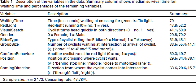
Description of the variables in the data. Summary column shows median survival time for WaitingTime and percentages of the remaining variables.

Variable	Description	Summary
WaitingTime	Time (in seconds) waiting at crossing for green traffic light.	79
RedLight	Red-light running (0 = no, 1 = yes).	47.8/52.2
VisualSearch	Cyclist turns head quickly in both directions (0 = no, 1 = yes).	41.1/58.9
Gender	0 = Female, 1 = Male.	29.8/70.2
RiderType	Type of cyclist riding the E-bike (0 = Normal, 1 = Takeaway).	51.9/48.1
GroupSize	Number of cyclists waiting at intersection at arrival of cyclist. (∈ {'none', '1 to 4' and ' 5 and more' }).	33.5/55.4/11.1
ConformBehaviour	Another cyclist runs the red light (0 = no, 1 = yes).	50.3/49.7
Position	Position at crossing where cyclist waits. (∈ {'behind stop line', 'middle', 'close to motorized lane'}).	29.5/34.4/36.1
ComingDirection	Direction from where the cyclist comes into intersection. (∈ {'through', 'left', 'right'}).	63.6/20.6/15.7
Sample size: n = 2173. Censoring rate: 47.78 %.

Table 2

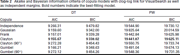
Akaike and Bayesian information criteria of copula models with clog-log link for VisualSearch as well as independent margins. Bold numbers indicate the best-fitting model.

Copula	DT		PW
	AIC	BIC	AIC	BIC
Independence	9266.31	9479.82	19544.90	19730.12
Gaussian	9159.60	9342.00	19825.64	20014.59
Frank	9157.01	9339.28	19442.84	19625.98
Clayton	9155.67	9338.02	19441.87	19625.11
Clayton (90∘)	9272.28	9454.43	19550.75	19733.74
Gumbel	9166.21	9348.63	19491.04	19674.13
Gumbel (90∘)	9272.12	9454.26	19548.36	19731.35

Figure 1

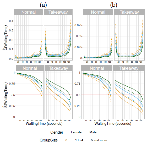
Estimated hazard rate and survival function across RiderType, GroupSize and Gender for DT (a) and PW (b) approaches. Red line indicates the median.

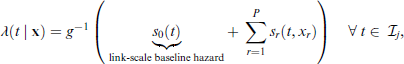
Using the augmented data, the log-likelihood of a DT model coincides with the Bernoulli log-likelihood (Tutz and Schmid, 2016). The discrete hazard is then $\lambda \left(j\mid x\right)={\vartheta }_j=g^{-1}\left({\eta }_j\right)$ , where ${\vartheta }_j\in \left[0,1\right]$ is the parameter of the Bernoulli distribution. If one follows a PW approach, the log-likelihood contribution coincides with the Poisson log-likelihood with offset $\text{ln}\left(t_j\right)=o_j$ , where $t_j$ is the time spent in the j-th interval (Bender et al., 2018). In this case, the hazard is $\lambda \left(j|x\right)=\text{exp}\left({\eta }_j\right)={\vartheta }_j/\text{exp}\left(o_j\right)$ , where ${\vartheta }_j=\text{exp}\left({\eta }_j\right)\text{exp}\left(o_j\right)$ is the parameter of the Poisson distribution. Note that both DT and PW approaches can accommodate time-dependent covariates, that is, $x_j$ . For either approach, a structured additive predictor is set as foundation for a regression model for the hazard rate:

$\lambda \left(t|x\right)=g^{-1}\left(\underset{\text{link-scale baseline hazard}}{\underbrace{s_0(t)}}+\sum _{r=1}^P{s}_r\left(t,x_r\right)\right)\forall t\in {\mathcal{I}}_j,$

where the baseline hazard is modelled as a smooth function of time and the functional form of the covariates can be any of those described in Section 2.1. For PW models $g\left(\cdot \right)$ is the natural logarithm function. In the DT framework, $g\left(\cdot \right)$ can be any suitable link function for for parameters with range $\left[0,1\right]$ , such as logit, probit and clog-log. We remark that our implementation currently features only the clog-log link but we plan to add others in the future. From a practical perspective, the clog-log link produces the 'grouped proportional hazards model', which can be seen as a discretized version of Cox's proportional hazards model (Tutz and Schmid, 2016).

3 Embedding DT and PW approaches into distributional copula regression

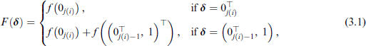
Using the DT or PW approach together with the augmented data, the i-th observation of the time-to-event margin is now represented by $j=1,\dots ,j\left(i\right)$ auxiliary variables, where $j\left(i\right)$ denotes the length of the sequence emanating from the i-th observational unit in the sample. We denote these as $\delta ={\left({\delta }_1,\dots ,{\delta }_{j\left(i\right)}\right)}^{\top }$ , which can have two possible expressions: $\delta =0_{j\left(i\right)}^{\top }$ in case of censoring or $\delta =\left(0_{j\left(i\right)-1}^{\top },1\right)$ in case of an event, that is, a non-censored observation, where $0_{j\left(i\right)}^{\top }$ and $0_{j\left(i\right)-1}^{\top },1$ denote zero vectors of length $j\left(i\right)$ and $j\left(i\right)-1$ , respectively.

We propose to use the following function based on the likelihood contributions of either DT or PW techniques:

$\begin{array}{c}F\left(\delta \right)=\left\{\begin{array}{ll}f\left(0_{j\left(i\right)}\right),\hfill & \text{if }\delta =0_{j\left(i\right)}^{\top }\hfill \\ f\left(0_{j\left(i\right)}\right)+f\left({\left(0_{j\left(i\right)-1}^{\top },1\right)}^{\top }\right),\hfill & \text{if }\delta =\left(0_{j\left(i\right)-1}^{\top },1\right),\hfill \end{array}\right.\end{array}$

(3.1)

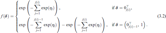
where $f\left(\delta \right)$ is the likelihood contribution for a right-censored or an observed time, respectively. Here we cumulate over the expressions $f\left(0_{j\left(i\right)}\right)$ and $f\left({\left(0_{j\left(i\right)-1}^{\top },1\right)}^{\top }\right)$ in case of an event, that is, $\delta =\left(0_{j\left(i\right)-1}^{\top },1\right)$ , to account for the auxiliary variables δ being discrete. The concrete expression of $f\left(\delta \right)$ depends on the adopted approach. For instance, choosing a DT model and setting the link function to the clog-log, that is, $\lambda \left(j\mid x\right)={\vartheta }_j=1-\text{exp}\left(-\text{exp}\left({\eta }_j\right)\right)$ , results in the following function based on the Bernoulli likelihood:

$$\begin{array}{c}f\left(\delta \right)=\left\{\begin{array}{ll}\text{exp}\left(-{\displaystyle \sum }_{j=1}^{j\left(i\right)}\text{exp}\left({\eta }_j\right)\right),\hfill & \text{if }\delta =0_{j\left(i\right)}^{\top }\hfill \\ \text{exp}\left(-{\displaystyle \sum }_{j=1}^{j\left(i\right)-1}\text{exp}\left({\eta }_j\right)\right)-\text{exp}\left(-{\displaystyle \sum }_{j=1}^{j\left(i\right)}\text{exp}\left({\eta }_j\right)\right),\hfill & \text{if }\delta =\left(0_{j\left(i\right)-1}^{\top },1\right).\hfill \end{array}\right.\end{array}$$

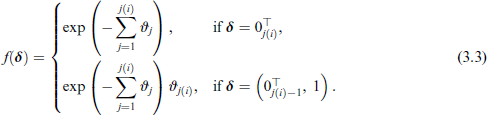
Using a PW approach, the conditional hazard corresponds to $\lambda \left(j\mid x\right)=\text{exp}\left({\eta }_j\right)={\vartheta }_j/\text{exp}\left(o_j\right)$ , leading to the following function based on the Poisson likelihood:

$\begin{array}{c}f\left(\delta \right)=\left\{\begin{array}{ll}\text{exp}\left(-{\displaystyle \sum }_{j=1}^{j\left(i\right)}{\vartheta }_j\right),\hfill & \text{if }\delta =0_{j\left(i\right)}^{\top },\hfill \\ \text{exp}\left(-{\displaystyle \sum }_{j=1}^{j\left(i\right)}{\vartheta }_j\right){\vartheta }_{j\left(i\right)},\hfill & \text{if }\delta =\left(0_{j\left(i\right)-1}^{\top },1\right).\hfill \end{array}\right.\end{array}$

We provide analytical first and second order partial derivatives of the proposed functions $f\left(\delta \right)$ and $F\left(\delta \right)$ based on DT and PW approaches with respect to a generic coefficient vector β in Supplementary Material B. These are required for the simultaneous estimation algorithm of our software implementation, which is based entirely on GJRM (Marra and Radice, 2023).

3.1 Bivariate additive copula regression for mixed non-time-to-event and time-to-event responses

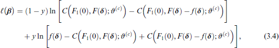
Recall that the bivariate non-commensurable outcome of interest is comprised of a non-time-to-event and a potentially right-censored time-to-event variable. We now replace the survival function of the potentially right-censored time-to-event margin with the proposed function $F\left(\mathit{\delta }\right)$ in Equation (3.1). Note that in this case Sklar's theorem is no longer used in its original form. We focus on cases when the non-time-to-event margin is binary, therefore the log-likelihood of the i-th observation has the following form (Marra et al., 2020):

$$\begin{array}{c}\mathcal{l}(\beta )=(1-y)\ln \left[C\left(F_1(0),F(\delta );{\vartheta }^{(c)}\right)-C\left(F_1(0),F(\delta )-f(\delta );{\vartheta }^{(c)}\right)\right]\\ +y\ln \left[f(\delta )-C\left(F_1(0),F(\delta );{\vartheta }^{(c)}\right)+C\left(F_1(0),F(\delta )-f(\delta );{\vartheta }^{(c)}\right)\right],\end{array}$$

(3.4)

where the copula C $(\cdot )$ is evaluated using the CDF of y at zero, that is, $F_1\left(0\right)$ and $F\left(\mathit{\delta }\right)$ .

Considerations for copula modelling: A crucial aspect of copula modelling is the fact that the dependence structure between the margins is preserved if a monotonic transformation is applied to them (Klement et al., 2002; Nelsen, 2006). If the proposed function $F\left(\mathit{\delta }\right)$ is a monotonic decreasing function of the time-to-event variable T, then the original dependence structure will be preserved and the use of our proposed approach would be justified. Otherwise, $F\left(\mathit{\delta }\right)$ will alter the original dependence structure, rendering our proposal not suitable for copula modelling. Supplementary Material A contains a proof that the proposed function $F\left(\mathit{\delta }\right)$ is a monotonic decreasing function of the original variable for both DT and PW approaches. Hence, replacing the survival function $S_2\left(t\right)$ with $F\left(\mathit{\delta }\right)$ in a bivariate copula model preserves the original dependence structure of interest. Additionally, we have conducted various simulation studies to assess the performance of the proposed approach using DT and PW likelihoods, these can be found in Supplementary Material D, available at https://journals.sagepub.com/home/smja . The R code used to conduct the simulations can be found in the following repository: https://github.com/GuilleBriseno/DTPW_DistCopulaReg.

4 Analysis of red-light running behaviour of E-cyclists

We study the behaviour of E-bike cyclists (E-cyclists) regarding traffic red-light running or traffic red light violation using a sample of n = 2173 subjects from Shanghai, China collected and previously analyzed by Gao et al. (2020). The margins of the bivariate mixed outcome consist of a binary non-time-to-event and a time-to-event variable, respectively. The binary response VisualSearch indicates whether a cyclist quickly turns their head in both directions while waiting at the crossing (0 = no, 1 = yes). This variable is considered a relevant factor in describing cyclists' red-light running and driving behaviour (Fraboni et al., 2018; Rupi and Krizek, 2019). The time-to-event variable WaitingTime gives the time in seconds until an E-cyclist crosses an intersection when the traffic light is red. The censoring indicator RedLight is equal to one if an E-cyclist runs the red-light and zero if they wait until the traffic light turns green. This means that those E-cyclists that arrived at the intersection during a red-light and only cross it until the signal turns green are treated as censored observations (Gao et al., 2020). This yields a censoring rate of 47.78%. It could be argued that those individuals that do not run the red traffic light in the data, that is, censored observations, will never commit such an infringement and should not be analyzed jointly with those that do so. However, we believe it is more reasonable to assume that any E-cyclist is capable of running a red traffic light under certain circumstances. Hence, for the censored observations in the sample, the conditions for violating the red traffic light were simply not met at the time of collecting the data and we assume that under different conditions such cyclists would cross an intersection given a red-light.

The covariates in the data describe three aspects of the E-cyclists: Individual characteristics, social influence and cycling information (Gao et al., 2020). Among the individual characteristics are the gender (female = 0, male = 1) of the cyclist and the factor variable RiderType which indicates whether the cyclist is a takeaway delivery driver or not. The social influence aspect is represented by two variables.

The categorical variable GroupSize, which says how many other cyclists were waiting at the intersection at the arrival of the subject ('none', '1 to 4 ' and ' 5 and more'), and ConformBehaviour which is equal to one if another cyclist runs the red light and zero otherwise. Social influence characteristics have been found to play an important role in decreasing the propensity of red-light running (Bai and Sze, 2020). Last the cycling information is described by the categorical variables Position and ComingDirection. Previous studies have found that Position plays an important role in determining driving behaviour (Tang et al., 2020). See Table 1 for a description of the variables.

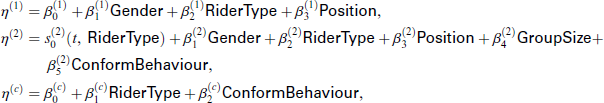
Model configuration: We aim to model the joint distribution of VisualSearch and WaitingTime using our proposed distributional copula regression approach. The binary response VisualSearch is modelled using a Bernoulli distribution with parameter ${\vartheta }^{\left(1\right)}\in \left[0,1\right]$ . The hazard rate of the time-to-event variable WaitingTime is modelled using the proposed functions based on the auxiliary variables $\mathit{\delta }$ using DT and PW approaches:

${(\text{VisualSearch },\text{WaitingTime })}^{\top }\sim C\left(F_1\left(\text{VisualSearch;}{\vartheta }^{\left(1\right)}\right),F\left(\delta ;\vartheta \right)|{\vartheta }^{\left(c\right)}\right),$

where $F_1(\cdot )$ is the CDF of the Bernoulli distribution and $F(\cdot )$ is the proposed function from Equation (3.1) with $\mathit{\vartheta }$ denoting the hazard rate built using either DT (clog-log link) or PW (natural logarithm link) methods. We omit the index k in the distribution parameters for the remainder of the article due to both margins depending only on one parameter. To construct the model of the hazard for WaitingTime, the follow-up is split using 20 intervals, resulting in intervals that are 6.5 seconds of length. We investigated alternative configurations with $\mathrm{130,65,35}$ and 13 intervals, but these did not change the results in a relevant way. The structured additive predictors of the model are:

$$\begin{array}{l}{\eta }^{(1)}={\beta }_0^{(1)}+{\beta }_1^{(1)}\text{ Gender }+{\beta }_2^{(1)}\text{ RiderType }+{\beta }_3^{(1)}\text{ Position,}\\ {\eta }^{(2)}=s_0^{(2)}(t,\text{ RiderType })+{\beta }_1^{(2)}\text{ Gender }+{\beta }_2^{(2)}\text{ RiderType }+{\beta }_3^{(2)}\text{ Position }+{\beta }_4^{(2)}\text{ GroupSize }+\\ {\beta }_5^{(2)}\text{ ConformBehaviour,}\\ {\eta }^{(c)}={\beta }_0^{(c)}+{\beta }_1^{(c)}\text{ RiderType }+{\beta }_2^{(c)}\text{ ConformBehaviour, }\end{array}$$

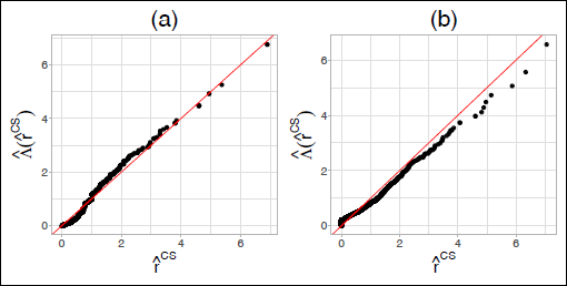
where the link-scale baseline hazard $s_0^{\left(2\right)}\left(\cdot \right)$ is modelled as a smooth function of time using P-splines with second order differences and is stratified depending on RiderType. Hence, we fit a separate baseline hazard for Normal and TakeAway E-cyclists. The remaining categorical covariates enter the model as linear effects with dummy coding. The dependence between the margins modelled via ${\eta }^{\left(c\right)}$ is allowed to change based on RiderType and ConformBehaviour. The variable ComingDirection is not included in the model due having no significant effect on any additive predictor. Note that the covariates were selected into the different additive predictors based on hypothesis testing (Marra and Radice, 2017). The copula function is selected out of the Gaussian, Frank, Clayton and Gumbel (with 90∘ rotations) copulas by means of the Akaike and Bayesian Information Criteria (AIC, BIC), see Table 2. We remark that GJRM supports more copula functions aside from the aforementioned, however we do not consider the entire catalogue in this article. All model coefficients are estimated simultaneously. Confidence intervals are obtained as described in Radice et al. (2016). The goodness-of-fit of δ is assessed using Cox-Snell residuals (Klein and Moeschberger, 2003) in Figure 2. Additional diagnostics of the fitted copula function can be found in Supplementary Material C2. The R code used to fit the models to the data can be found in the following repository: https://github.com/GuilleBriseno/DTPW_DistCopulaReg .

Figure 2

Cox-Snell residuals corresponding to the model of WaitingTime using the DT (a) and PW (b) approaches.

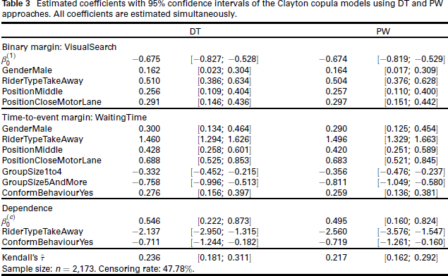
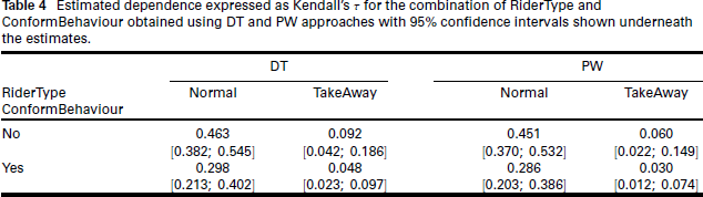
Results using DT approach: The best fitting model is a Clayton copula with clog-log link for VisualSearch, the estimated coefficients are shown in the DT column of Table 3. The column corresponding to the DT models in Table 2 shows that the Clayton copula fits the data better compared to using independent margins. We find that on average there exists a significant 'moderate' positive dependence between VisualSearch and WaitingTime with Kendall's τ estimated at $\widehat{\tau }=0.236\left[0.181,0.311\right]$ with $\alpha =0.05$ . The additive predictor of the dependence parameter ${\eta }^{\left(c\right)}$ decreases for takeaway relative to normal cyclists. A less pronounced decrease in the predictor ${\eta }^{\left(c\right)}$ is also observed when another cyclist at the intersection commits a red traffic light violation (ConformBehaviour = 1). These estimates indicate that the behaviour of E-cyclists is influenced by social or group factors while waiting at an intersection. Table 4 shows the values of the estimated Kendall's τ for the combinations of the binary variables RiderType and ConformBehaviour. It can be seen that the dependence between the margins decreases for takeaway cyclists whenever there is conforming behaviour. Comparatively, the estimated dependence between VisualSearch and ConformBehaviour is much stronger for normal cyclists and when no other driver crosses the junction. Regarding the model for VisualSearch, takeaway cyclists have on average a significantly higher probability of checking for traffic in both directions relative to normal cyclists, ceteris paribus. On average, male cyclists also have a significantly higher change of conducting VisualSearch relative to female cyclists, ceteris paribus. Figure 1 shows the estimated hazard rate and corresponding estimated survival function from the Clayton model based on different values of GroupSize and RiderType. Overall, a noticeable shift upwards in the hazard rate can be seen for takeaway cyclists. Conversely, the estimated survival function for takeaway cyclists lies below the one corresponding to normal cyclists. This phenomenon depicts the riskier behaviour that delivery-service cyclists exhibit to meet demand in the delivery-service industry (Gao et al., 2020; Zhang and Liu, 2023).

Table 3

Estimated coefficients with 95% confidence intervals of the Clayton copula models using DT and PW approaches. All coefficients are estimated simultaneously.

		DT		PW
Binary margin: VisualSearch
${\beta }_0^{\left(1\right)}$	-0.675	[-0.827; -0.528]	-0.674	[-0.819; -0.529]
GenderMale	0.162	[0.023; 0.304]	0.164	[0.017; 0.309]
RiderTypeTakeAway	0.510	[0.386; 0.634]	0.504	[0.376; 0.628]
PositionMiddle	0.256	[0.109; 0.404]	0.257	[0.110; 0.400]
PositionCloseMotorLane	0.291	[0.146; 0.436]	0.297	[0.151; 0.442]
Time-to-event margin: WaitingTime
GenderMale	0.300	[0.134; 0.464]	0.290	[0.125; 0.454]
RiderTypeTakeAway	1.460	[1.294; 1.626]	1.496	[1.329; 1.663]
PositionMiddle	0.428	[0.258; 0.601]	0.420	[0.251; 0.589]
PositionCloseMotorLane	0.688	[0.525; 0.853]	0.683	[0.521; 0.845]
GroupSize1to4	-0.332	[-0.452; -0.215]	-0.356	[-0.476; -0.237]
GroupSize5AndMore	-0.758	[-0.996; -0.513]	-0.811	[-1.049; -0.580]
ConformBehaviourYes	0.276	[0.156; 0.397]	0.259	[0.136; 0.381]
Dependence
${\beta }_0^{\left(c\right)}$	0.546	[0.222; 0.873]	0.495	[0.160; 0.824]
RiderTypeTakeAway	-2.137	[-2.950; -1.315]	-2.560	[-3.576; -1.547]
ConformBehaviourYes	-0.711	[-1.244; -0.182]	-0.719	[-1.261; -0.160]
Kendall's $\hat{\tau }$	0.236	[0.181; 0.311]	0.217	[0.162; 0.292]
Sample size: n = 2,173. Censoring rate: 47.78%.

The GroupSize covariate describes the social behaviour of the cyclist while waiting for green traffic light. The magnitude of the estimated effect on the link-scale hazard rate increases based on the level of GroupSize. Hence, the more individuals waiting at the crossing or the more crowded the crossing becomes, the less likely that the cyclist will violate the traffic red-light. Figure 1 column (a) depicts the estimated hazard rates and survival functions based on the DT approach. The effect of GroupSize can be seen to produce a shift downwards in the estimated hazards and upwards in the estimated survival functions. The estimated survival functions shown in Figure 1 column (a) exhibit different patters for normal and takeaway cyclists, respectively. It can be seen that the median survival time is dramatically lower for takeaway cyclists. The estimated hazard rate shown in Figure 1 column (a) shows that the hazard for takeaway E-cyclists has a 'U' or bathtub shape. This means that the risk of violating the red traffic light is higher at the cyclist's arrival at the intersection as well as close to the end of the red signal. The Cox-Snell residuals shown in Figure 2 (a) corresponding to the DT approach indicate that the fitted model with a stratified baseline hazard for RiderType fits the data well. Table C1 and Figure C1 in Supplementary Material C show the estimated coefficients as well as the estimated hazard and survival functions, respectively, when assuming independence between the margins. Overall, the estimated coefficients from univariate independent models exhibit some differences in their magnitude, but a similar trend can be seen for all of the considered covariates. The diagnostics regarding the fitted Clayton copula function in Supplementary Material C indicate that although the Clayton copula performs best among the considered parametric copula families, asymmetry can be seen in the joint tail dependence. Figure C2 in Supplementary Material C indicates that a parametric copula family likely struggles to adequately model the dependence between the margins. Histograms of the margins $F_1$ (VisualSearch) and $F\left(\delta \right)$ shown in Figure C 4 (a) show that the margin $F\left(\delta \right)$ does not resemble a uniform distribution, indicating that the fit of the lower tail of the aforementioned margin could be improved.

Table 4

Estimated dependence expressed as Kendall's τ for the combination of RiderType and ConformBehaviour obtained using DT and PW approaches with 95% confidence intervals shown underneath the estimates.

RiderType ConformBehaviour	DT		PW
	Normal	TakeAway	Normal	TakeAway
No	0.463 [0.382; 0.545]	0.092 [0.042; 0.186]	0.451 [0.370; 0.532]	0.060 [0.022; 0.149]
Yes	[0.213; 0.402]	[0.023; 0.097 ]	[0.203; 0.386]	[0.012; 0.074]

Results using PW approach: According to Table 2, the best-fitting copula is once again the Clayton copula. In addition, the column PW in Table 2 shows that the Clayton copula model delivers a better fit compared to fitting independent univariate margins. The estimated coefficients for the model based on the PW approach closely resemble those of the DT approach. The 95% confidence intervals shown in Table 3 are also very similar for both approaches. The estimated dependence quantified as Kendall's τ is also close to the DT approach-based model, sitting at $\widehat{\tau }=0.217\in \left[0.162;0.292\right]$ . See Table 4 for the estimated values of Kendall's τ for every combination of RiderType and ConformBehaviour. Once again, the estimated values resemble that of the model based on the DT approach. The estimated hazard rates and survival functions shown in Figure 1 (b) exhibit the same pattern as those based on the DT approach. The Cox-Snell residuals from Figure 2 (b) also suggest that the PW-based model fits the data well apart from some outliers in the upper tail of the data. The results from fitting independent univariate models shown in Table C1 and Figure C1 in Supplementary Material C exhibit some changes in the magnitude of the estimated coefficients. Similar trends to those found in the copula models can be observed. The diagnostics regarding the Clayton copula from Supplementary Material C point towards similar conclusions as those drawn from the DT approach, where asymmetry can be seen in the joint tail dependence. In addition, Figure C4 (b) in Supplementary Material C shows that the fit of lower tail of the margin $F\left(\delta \right)$ can be improved. One possible solution to accommodate the aforementioned asymmetry while keeping a parametric model for the dependence would be to implement Khoudraji's device (Genest et al., 1998). This approach modifies parametric copula functions by introducing one or two scalar asymmetry parameters. Another option would be to pursue a non-parametric approach, such as using kernel density-based bivariate copulas, as proposed in Nagler and Czado (2016). This approach would have the advantage of being more flexible than the parametric copula families considered so far. However, these are outside of the scope of this article.

5 Discussion

We have proposed a distributional regression model that embeds DT as well as PW modelling approaches into a copula regression framework for bivariate mixed outcomes. This allows to cast highly flexible regression models for the hazard rate of the time-to-event margin, which can include smooth functions of time, time-dependent covariates as well as time-varying effects. From a computational point of view, since our regression model for the time-to-event margin is based on the hazard rate, it does not require any constraints on the estimated smooth functions of time. Hence, we can avoid adding penalties or reparameterisations to impose such constraints, for example, that the baseline function of time must be monotonically decreasing, see Liu et al. (2018) and Marra and Radice (2019) for more details. The data transformation into long format depends on the configurations set by the analyst. Instead of treating the number of intervals as a tuning parameter, we suggest to set the number of intervals that cut the follow-up to a rather large value (e.g. 20 intervals) and let the penalty term of the baseline hazard take care of the compromise between overfitting the data and smoothness of the estimated function.

We embedded the DT and PW approaches into a bivariate distributional copula regression framework and implemented them in the convenient open source R library GJRM, allowing practitioners to cast flexible statistical models for mixed outcomes as well as bivariate time-to-event (implemented, but not presented here). Although not shown in this article, the proposed approach can also be used for modelling bivariate right-censored time-to-event responses as in Marra and Radice (2019), using DT or PW methods. This would involve modifying the log-likelihood to one based on bivariate discrete data shown in van der Wurp et al. (2020). We have demonstrated the versatility of the proposed approach by analysing the joint bivariate distribution of a non-commensurable outcome that consisted of binary and time-to-event margins using DT and PW approaches. The analysis showed that takeaway E-cyclists have a higher propensity to conduct a visual search, that is to inspect both directions of an intersection, as well as to run traffic red lights compared to normal E-cyclists. The model shows a moderately strong estimated dependence between visual search and the time to red-light running for all E-cyclists. Our results also show that the red-light running of another cyclist waiting at the same intersection decreases the dependence between the responses.

Our approach has several potential avenues for future developments. One of them would be to adapt our software implementation to support other non-time-to-event margins such as ordinal outcomes following Hohberg et al. (2021). Another aspect could be the inclusion of a cure fraction (i.e. cure models, Peng and Yu, 2021) to account for subjects that will never experience the event. This phenomenon appears to be present in the data analyzed in Section 4, where cyclists that did not violate the traffic light are considered censored observations. Instead, one could argue that those cyclists belong to a sub-population that does not commit such infractions. An indication of the presence of such a cure fraction can be seen in the fact that the estimated survival function of normal (non-takeaway) E-cyclists remains far from zero. Thus, there may be E-cyclists that 'never' violate red traffic lights. We may consider relaxing the assumption of non-informative censoring times and model their distribution similar to Dettoni et al. (2020). Alternatively, we could explore relaxing the assumption of independent censoring and allow for dependent censoring as in Czado and Van Keilegom (2022). By doing so we would need to not only account for the dependence between the margins but also between the censoring and event times, which would result in a model that uses two copula functions. Another potential extension is modelling recurrent events based on Ramjith et al. (2022), which could require modifications of the proposed PW functions, but it would greatly extend the applicability of our methods. Data-driven variable selection could be tackled, for example, using a quadratic approximation of LASSO-type penalized models as in van der Wurp and Groll (2021) or boosting for distributional copula regression following Hans et al. (2022) and Strömer et al. (2023). Last, more flexible types of copula functions could be explored. For instance, Khoudraji's device (Genest et al., 1998) allows to model asymmetry in the dependence or alternatively a fully non-parametric approach could be pursued for modelling the dependence between the margins in cases where parametric copula families struggle to accommodate the data. These type of copulas are an attractive candidate for future work due to their parametric nature.