
Abstract
We address the challenge of correlated predictors in high-dimensional generalized linear model (GLMs), where regression coefficients range from sparse to dense, by proposing a data-driven random projection (RP) method. This is particularly relevant for applications where the number of predictors is (much) larger than the number of observations and the underlying structure—whether sparse or dense—is unknown. We achieve this by using ridge-type estimates for variable screening and RP to incorporate information about the response–predictor relationship when performing dimensionality reduction. We demonstrate that a ridge estimator with a small penalty is effective for RP and screening, but the penalty value must be carefully selected. Unlike in linear regression, where penalties approaching zero work well, this approach leads to overfitting in non-Gaussian families. Instead, we recommend a data-driven method for penalty selection. In a simulation study, this data-driven RP improved prediction performance over conventional RPs, even surpassing benchmarks like elastic net. Furthermore, an ensemble of multiple such RPs combined with probabilistic variable screening delivered the best aggregated results in prediction and variable ranking across varying sparsity levels in our simulation study at a rather low computational cost. Final, three applications with count and binary responses demonstrate the method’s advantages in interpretability and prediction accuracy.
Keywords
Introduction
High-dimensional data in a regression context, where the number of variables exceeds the number of observations (i.e., p > n or even
The generalized linear model (GLM) extends the linear model to both continuous and discrete responses while maintaining interpretability. In high-dimensional settings, GLMs are typically regularized (e.g., Tibshirani, 1996; Fan and Li, 2001; Zou and Hastie, 2005). Alternatively or complementarily, the dimensionality of the feature space can be reduced to a moderate size while learning and inference is performed in this reduced predictor space. One fast way to achieve this is variable screening, that is, selecting a subset of the predictors based on their utility. Methods for screening often rely on parametric (such as the maximum likelihood estimates of univariate GLMs, Fan et al., 2009; Fan and Song, 2010) or nonparametric (e.g., Fan et al., 2011; Mai and Zou, 2013, 2015; Ke, 2023) measures but typically ignore predictor correlations. Fan et al. (2009) suggest an iterative procedure to address this issue, while Wang and Leng (2016) propose screening variables in linear regression using the high-dimensional ordinary least squares projection (HOLP), a ridge-type estimator with a closed form solution when the penalty converges to zero. However, screening approaches based on ridge-type estimators are still rare in the context of GLMs.
An approach similar in scope to variable screening is random projection (RP), which reduces the dimensionality of the feature space by linearly projecting the features onto a lower-dimensional space, rather than employing a reduced set of the original features. Conventional RPs contain i.i.d. entries from a suitable distribution and are oblivious to the data to be used in the regression. Such projections have been used in a classification setting, for example, by Cannings and Samworth (2017), while Guhaniyogi and Dunson (2015); Mukhopadhyay and Dunson (2020) focus on linear regression. On the other hand, Ryder et al. (2019) propose a data-informed RP using an asymmetric transformation of the predictor matrix without using information of the response. Parzer et al. (2025) propose a data-driven projection for linear regression which incorporates information from the estimated HOLP coefficients, that is, about both the predictors and the response.
In this article, we leverage the computational advantages of variable screening and RP and introduce a data-driven RP method for GLMs that accounts for the relationship between predictors and the response, while addressing the potentially complex correlation structure among the predictors. The manuscript extends Parzer et al. (2025) to the GLM family of models, by proposing a ridge-type estimator which can be integrated into a sparse RP matrix and can also be employed for screening the variables prior to projection, as it performs well in preserving the true relationship between predictors and the response.
A key aspect of the proposed ridge-type estimator is the selection of the penalty term. We extend the HOLP estimator to GLMs with canonical link, deriving a closed-form solution and explore if it retains the same benefits for RP and screening in GLMs as in linear regression. We find that for non-Gaussian families, a ridge estimator with zero penalty can overfit, making penalty selection a non-trivial task. While small penalty values reduce bias, a data-driven approach to choosing the penalty works best. Specifically, we propose selecting the smallest penalty value for which the deviance ratio in the fit stays under a certain threshold (e.g., 0.8 for non-Gaussian families and 0.999 for Gaussian). Simulations show that using these ridge estimates in the sparse RP matrix outperform conventional RP techniques.
Given the randomness in the RP matrix, variability can be reduced by building ensembles of multiple RPs. For example, Guhaniyogi and Dunson (2015) propose repeatedly sampling RPs of different sizes and estimating an ensemble of linear regressions on the reduced predictors, while Cannings and Samworth (2017) generate various RPs for each classifier in an ensemble and pick the best one based on an appropriate loss function. Additionally, ensembles of multiple RPs and variable screening steps have also been proposed that achieve better predictive performance in linear regression (Mukhopadhyay and Dunson, 2020; Parzer et al., 2025).
In a similar fashion, we extend the variable screening and RP procedure by building an ensemble of GLMs and averaging them to form the final model, adapting the algorithm in Parzer et al. (2025) to GLMs. An extensive simulation study reveals that this ensemble improves predictive performance, ranks predictors effectively and is computationally efficient, particularly with increasing predictor dimensions. It consistently performs well against state-of-the-art approaches such as penalized regression, random forests and support vector machines (SVMs) across a range of sparsity settings and yields the best overall performance when aggregated across all scenarios. This broad applicability makes the method versatile for high-dimensional regression with correlated predictors, especially when the sparsity of the underlying data-generating process is unknown and capable of computationally handling datasets with small n and a (very) large number of predictors.
The integration of the GLM framework with probabilistic screening improves model interpretability, as the coefficients in the marginal models can be extracted and their reliability and relevance can be assessed. The GLM framework also offers modeling flexibility, facilitating seamless comparison across different family–link combinations.
The article is organized as follows: Section 2 presents the GLM model, data-informed RP, variable screening and the ensemble algorithm. Section 3 provides simulations comparing the method with state-of-the-art approaches. Applications are shown in Section 4 and Section 5 concludes.
Method
This section begins by presenting the GLM model class, followed by an introduction to the dimension reduction tools RP and variable screening. Then, we propose a novel coefficient estimator useful for both these concepts and state how this estimator can be used to extend the algorithm in Parzer et al. (2025) to GLMs. Throughout the section, we use the notation
Generalized linear models
We assume to observe high-dimensional data

where θi is the natural parameter, a(.) > 0 and c(.) are specific real-valued functions determining different families, ϕ is a dispersion parameter and b(.) is the log-partition function normalizing the density to integrate to one. If ϕ is known, we obtain densities in the natural exponential family for our responses. It can be shown that b(.) is twice differentiable and convex with
The responses are related to the p-dimensional predictors through the conditional mean, that is, the conditional mean of yi given

where
but for maximization with respect to β, it suffices to use

and treat ϕ as a nuisance parameter. In our general high-dimensional setting p > n, the predictor matrix
RP can be used as a dimension-reduction tool for high-dimensional regression by creating a random matrix
When using random sign diagonal elements
Variable screening aims at selecting a small subset of variables based on some marginal utility measure and using the ones with the highest utility for further analysis. This procedure can complement the RP approach and further reduce the dimensionality of the problem by first screening for the important variables and then performing the RP. A seminal contribution in variable screening is the sure independence screening (SIS) of Fan and Lv (2008), who proposed to use the absolute marginal correlation of the predictors to the response in linear regression, which was later extended to GLMs in Fan et al. (2009); Fan and Song (2010) by employing the maximum likelihood coefficient estimates of univariate GLMs instead of the correlation coefficient. However, in the presence of predictor correlation, screening based on a conditional utility measure (i.e., conditional on all the other variables in the model) is to be preferred to the unconditional one. To tackle this issue, Fan and Lv (2008) propose iterative SIS, which involves iteratively applying SIS and penalized regression to select a small set of variables, computing the residuals of a model fitted with the selected variables and using these residuals as a response variable to continue finding relevant variables. This procedure was later extended to more general model classes in Fan et al. (2009).
Similar to the linear regression case, the absolute value of the true coefficients in a GLM (assuming all predictors have the same scale) can be employed as a measure of variable importance. Therefore, another approach is to find a screening coefficient that is capable of detecting the correct order of magnitudes of the regression coefficients (but not necessarily their signs). We note that an estimator that performs well for the purpose of RP (as discussed above) would also be a good candidate as a screening coefficient. In the next section, we propose such an estimator for GLMs.
Proposed estimator for random projection and screening
In general, a ridge-type estimator

with the scaled log-likelihood

where
Motivated by (2.5) and Kobak et al. (2020), who showed that the optimal ridge-penalty in linear regression can be negative due to implicit regularization from high-dimensional predictors, we first investigate whether

for
The proof can be found in the Supplementary Materials A. The intercept-free assumption can be avoided by appropriate centering of
As an alternative that can cover all cases, we propose to approximate
Furthermore, in order to understand whether more penalization (i.e., through higher values of λ) is needed for other families as compared to the Gaussian case, we investigate alternative strategies for choosing the penalty value. In a simulation example in Section 3.3, we investigate the choice of this λmin for different families. It shows that for non-Gaussian families, it is beneficial to use a higher λmin to avoid a saturated fit. We also show that the resulting estimator allows good recovery of sign and magnitude of the true non-zero coefficients, while also performing well in terms of prediction when employed in the RP matrix.
Employing a single data-driven RP with the proposed estimator and then estimating a GLM on the reduced predictors can lead to high variability due to randomness. We address this by adapting the Sparse Projected Averaged Regression (SPAR) algorithm from Parzer et al. (2025) to GLMs, which builds an ensemble of GLMs in the following way: (a) randomly sampling predictors for inclusion in the RP based on the proposed screening coefficient, (b) projecting the sampled variables to a randomly chosen lower dimension using the proposed RP, (c) estimating penalized GLMs with the reduced predictors and (d) averaging them to form the final model. The adapted algorithm is given below, where * indicates changes compared to the linear regression formulation:
1.* Choose family with corresponding log-likelihood ℓ(.) and link and standardize covariate inputs 2.* Calculate 3. For k = 1, …, M:
3.1. Draw 2n predictors with probabilities 3.2. Project remaining variables to dimension mk randomly drawn with 3.3.* Fit a GLM of 4. For a given threshold ν ≥ 0, set all entries 5. Combine via simple average on link-level 6. Optionally, select M and ν via cross-validation by evaluating a two-dimensional grid of values. For each training fold, repeat Steps 2–6 using fixed index sets 7. Output the estimated coefficients and predictions for the chosen M and ν.
Our goal is to select the smallest penalty that maintains good predictive performance in the context of screening and RP for GLMs. In our experiments, the estimator in Equation (2.6) (or its approximation) does not consistently achieve the best predictive performance across all family–link function combinations. The strategy for selecting the penalty parameter λmin is detailed in Section 3.3. Specifically, we recommend choosing the smallest λ for which the deviance ratio remains below a predefined threshold. Using a threshold on the deviance ratio has the advantage of being invariant to the data scale and link function.
In Step 3.2 the dimension mk is random for the purpose of introducing more variability in the ensemble and reducing the reliance on a fixed (possibly arbitrarily chosen) goal dimension, in line with previous literature (e.g., Mukhopadhyay and Dunson, 2020).
In fitting the marginal models in Step 3.3, we also obtain intercept estimates, which can also be averaged and translated back to the original predictor scale to give an overall estimate
This algorithm allows for several variations: (a) Different measures can be used in the cross-validation, such as mean squared error instead of the family-dependent deviance. (b) If more sparsity in the coefficients is desired, (M, ν) can be chosen by the one-standard-error rule, which yields the sparsest
Simulation study
In a first simulation study, we compare how well the estimator (2.4) recovers the true active β across different penalty choices and evaluate the predictive performance of the data-driven RP with these estimators. We then compare SPAR algorithm’s predictive performance and variable ranking ability against various benchmarks in a comprehensive simulation study.
Setup
We generate data from Equation (2.1) for five family–link combinations with n = 200 and use additionally ntest = 1 000 observations as a test sample. The p-dimensional predictors are simulated as
We consider p = 500, 2 000, 10 000 and three sparsity settings for β: sparse (a = [2 log(p)]), medium (a = [2 log(p) + n/2]) and dense (a = p/4), where a is the number of non-zero entries in β. These entries are independently set as
Measures
Prediction performance is assessed on the independent test samples

where

where
Furthermore, we evaluate variable ranking performance using the partial AUC (pAUC) where the true binary labels indicate whether a variable is truly active and the absolute estimated coefficients serve as ranking scores. To ensure fair comparison between sparse methods and dense methods, we limit the number of false positive to n/2 (see Wang et al., 2019), implicitly limiting the false positive rate to n/(2(p − a)) with p − a truly inactive variables. To obtain an interpretable measure in the interval (0, 1), we divide the resulting pAUC by n/(2(p − a)) so that a perfect method would obtain a pAUC of 1.
Simulations for screening and random projection
Recovery of true active β
We investigate whether the ridge estimator in (2.4) is appropriate for the purpose of screening and data-informed RP in the sense that it is able to recover the true active coefficients well by considering the correlation to the true active β.
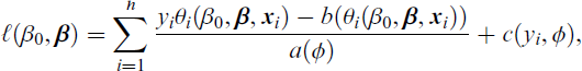
In the following, we present results for the scenario n = 200, p = 2 000 and The screening coefficient in Fan and Song (2010), where each βj is estimated by the slope of a marginal GLM (marGLM) with an intercept and only one predictor Ridge estimator from (2.4) with λ chosen by cross-validation based on the deviance criterion (L2_cv) Ridge estimator from (2.4) with λ converging to zero (L2_limit0). In the binomial–logit case, we use the exact limit for Ridge estimator with a data-driven approach to choosing λ as the smallest value for which the fraction of (null) deviance explained does not exceed 60% (L2_dev06), 80% (L2_dev08), 95% (L2_dev095) and 99.9% (L2_dev0999). Fixed deviance thresholds are used instead of fixed λ values, since the latter varies strongly across families. Table 2 in the Supplementary Materials shows average λ resulting from the cross-validation and the deviance cut-offs; higher deviance cut-offs lead to smaller λ, with large variation in the actual values across families.
Figure 1 shows the distribution of the correlation coefficient of the true active coefficients to different screening coefficients over 100 replications. We observe that L2_limit0 did not deliver the best results for all investigated family–links (for conciseness, we omit the results for binomial–cloglog as they are similar to binomial–logit). L2_cv also underperformed and the marGLM coefficients were the least effective at recovering the true coefficients. For binomial, differences among the ridge estimators were minor, but for Poisson, the performance declined as the deviance ratio threshold increases or λ becomes too small. While the cross-validated penalty seems to be too large for the purpose of screening, using a 0.8–0.95 deviance ratio for non-Gaussian families and 0.999 for Gaussian responses yields good results. The corresponding estimates are therefore well-suited as diagonal elements approximately proportional to the true β in our data-informed RP from Definition 2.1. In this comparison, we also computed the pAUC of these coefficients and the ratio of true active variables within the highest 3a absolute estimated values, but omitted these results as they are similar to those based on correlation.
Correlation of true active coefficients to different screening estimators for 100 replications (n = 200, p = 2 000, medium sparsity and block-diagonal Σ ).
Correlation of true active coefficients to different screening estimators for 100 replications (n = 200, p = 2 000, medium sparsity and block-diagonal Σ ).
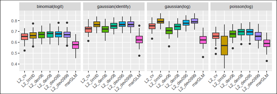
Next, in the same setting as above, we investigate the predictive performance of a model where the predictors are first projected onto a m = n/4 = 50 lower-dimensional space using the proposed data-informed RP with different screening coefficients, namely L2_cv, L2_limit0, L2_dev06, L2_dev08, L2_dev095 and L2_dev0999 from the previous section. Additionally, we also show the oracle performance of our proposal using the true β in the RP (True_Beta). We also consider models where conventional RPs (i.e., Gaussian with iid standard normal entries and SparseCW, the matrix from Definition with random sign diagonal elements) are used. Furthermore, we estimate the models with adaptive LASSO (AdLASSO; Zou, 2006) and elastic net (α = 1/2) with penalty chosen by cross-validation based on deviance (ElNet) as performance benchmarks.
In Figure 2, we present the rMSLE and the prediction error (1 AUC for binomial, rMSPE for Gaussian and Poisson) for ntest = 1 000 over 100 repetitions and see that the proposed data-informed projection with ridge estimates in the diagonal generally increases the performance with respect to both metrics over the conventional RPs (Gaussian and SparseCW), reaching a lower link estimation error and prediction error. The differences between the ridge estimators are less obvious, but generally, we see that the performance of the estimators in terms of screening also translates to the prediction power, namely that L2_dev0999 or L2_limit0 deliver the best results for the Gaussian family with both identity and log link, while L2_dev08 and L2_dev095 achieve the best prediction performance for the other families. Furthermore, for this example, it can be seen that this adaptation of the diagonal of the projection matrix suffices to reach a better performance than high-dimensional regression benchmarks, adaptive LASSO and elastic net, but there is a noticeable gap to the oracle performance.
We note that we assessed the sensitivity of the results in Figure 2 regarding the choice of the goal dimension m = n/4 but observed that results are stable for values of m between log(p) and n/2 (see also Figure 9 in the Supplementary Materials).
Link estimation error (MSLE) and prediction error (1 − AUC for binomial, MSPE otherwise) for 100 replications (n = 200, p = 2 000, medium sparsity, block Σ ). All projected methods use a single projection (without screening or ensembling).
Link estimation error (MSLE) and prediction error (1 − AUC for binomial, MSPE otherwise) for 100 replications (n = 200, p = 2 000, medium sparsity, block Σ ). All projected methods use a single projection (without screening or ensembling).
We consider n = 200, p = 2 000 in sparse, medium and dense settings for the five family–link combinations and a block structure for
We compare the following methods. As GLM-based methods, we use LASSO, elastic net (ElNet; α = 1/2), ridge, adaptive LASSO ((AdLASSO; using package glment by Tay et al. 2023) and SIS (Fan and Song, 2010). The penalty in the GLM-based methods is chosen by cross-validation using deviance and by employing the one-standard-error rule. Then, as general regression benchmarks, we use random forest (RF implemented R-package
Final, as a set of methods using RPs, we use an ensemble of 50 models with the conventional RP from Definition with random sign entries without any screening and random goal dimensions as in Step 3.2 of the SPAR algorithm in Section 2.4 (RP_CW_Ensemble), Targeted Random Projections (TARP), which is an adaptation of Mukhopadhyay and Dunson (2020) to GLMs where we perform screening based on marginal GLM coefficients and use the conventional RP of Achlioptas (2003) with ψ = 1/6 for an ensemble of M = 20 models, as well as our proposed SPAR algorithm from Section 2.4 in two configurations: (a) Without cross-validation, using a fixed number of M = 20 models and selecting the thresholding parameter ν from a predefined grid of 20 values (starting at 0 and followed by quantiles of the absolute values of all non-zero standardized coefficients, computed at evenly spaced probability levels from 1/(20 1) to 1) based on the best model deviance on the training set; and (b) with cross-validation over a grid of 20 ν values and a grid M = 10, 20, 30, 50 models. For both SPAR methods, the screening coefficient is the L2_dev08 for binomial and Poisson family and L2_dev0999 for Gaussian family. Furthermore, link-level averaging is employed in the ensembles, as it has the advantage of preserving the interpretability of the coefficients.
Predictive performance
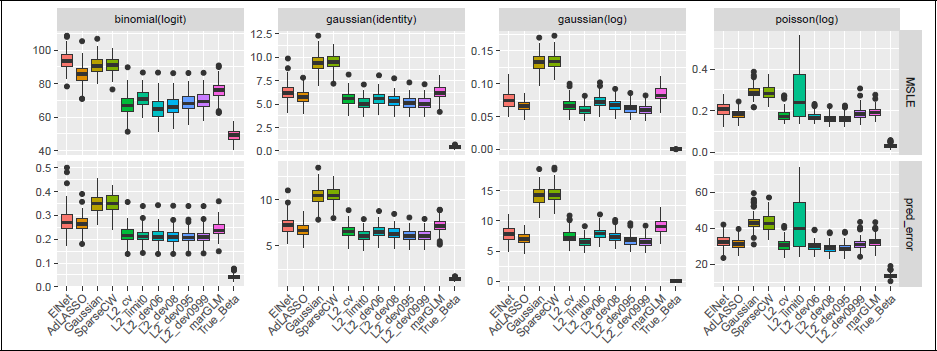
Figure 3 shows prediction and link estimation performance for 100 replications of n = 200, p = 2 000 in the block covariance setting. LASSO and SIS are excluded for brevity, as they were consistently outperformed by AdLASSO and elastic net, respectively. For the binomial family, we consider 1 AUC as the prediction error, for all other families the rMSPE. AUC is a measure of discrimination power rather than calibration (i.e., how well the probabilities are estimated). For measuring calibration, the rMSPE (scaled Brier score) can be employed. While the choice of the prediction measure is highly dependent on the application context, we note that the Brier score will be more sensitive than the AUC to the type of averaging in the ensemble methods (link versus response-level averaging). Note that, even if the link estimation is excellent, especially probabilities in the tails of the distribution can be over/underestimated by averaging on the link level, given the non-linear link function. We therefore consider AUC as the prediction measure in the subsequent analysis but provide results with rMSPE and AUC for the binomial family in different settings, as well as results for SPAR using response-level averaging, in Figure 11 in the Supplementary Materials.
Comparison of prediction performance (1 − AUC for binomial family, rMSPE for all other families) and link estimation (rMSLE, not reported for SVM and RF) over 100 repetitions (n = 200, p = 2 000, medium sparsity and block Σ ).
Comparison of prediction performance (1 − AUC for binomial family, rMSPE for all other families) and link estimation (rMSLE, not reported for SVM and RF) over 100 repetitions (n = 200, p = 2 000, medium sparsity and block Σ ).
Generally, SPAR and SPAR-CV were among the best-performing methods in all settings, except the sparse ones, where it was outperformed by AdLASSO and elastic net in terms of prediction and link estimation. In particular, SPAR seems to inherit strong prediction performance in dense cases from the L2-estimator in the screening (also used in the RP), while yielding stronger predictions compared to dense methods in medium and sparse settings. Especially, the performance in link estimation for the logistic regression is remarkable.
Comparison of variable ranking (pAUC rescaled to [0, 1] for better comparison) over 100 repetitions for n = 200, p = 2 000, medium sparsity and block Σ .
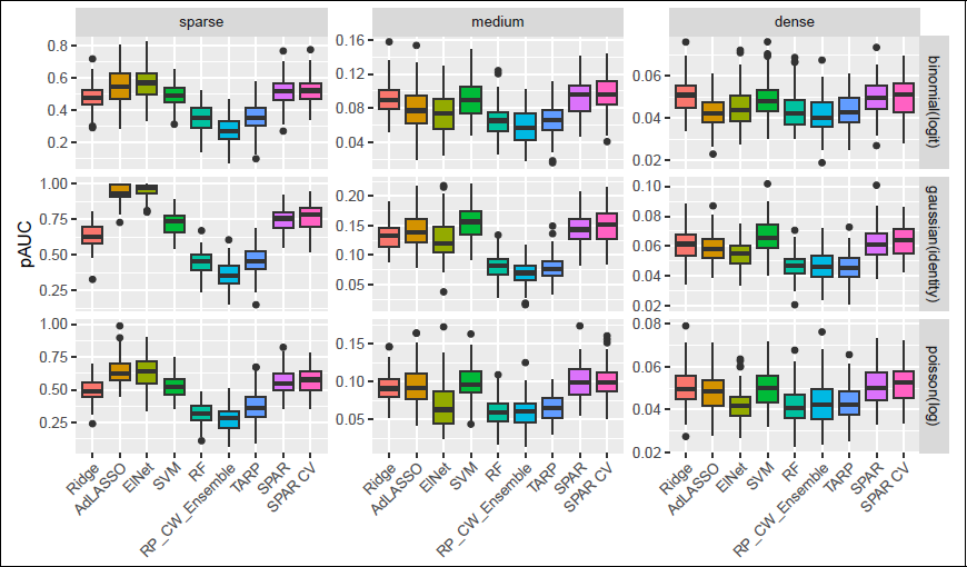
Figure 10 in the Supplementary Materials provides further results for prediction error for the five family–link combinations across the different covariance settings in the medium setting and p = 2 000 as well as for increasing p in the block covariance and medium sparsity. Results for AR(1) and block covariance were similar in both prediction performance and method ranking. All methods performed best under compound symmetry and worst under independence, likely reflecting the information content in the covariance. SPAR and SPAR CV are (among) the best methods for all covariance settings, except for the Poisson family in the compound symmetry and independent covariance settings. Compared to the block or ar1 setting, SVM performed worse under compound symmetry, except for the Gaussian identity case, while RF ranked higher for compound symmetry and independent settings, particularly for Gaussian and Poisson families. Performance declined with increasing dimensionality, with adaptive LASSO and elastic net most affected.
Figure 4 shows that SPAR and SPAR-CV both perform well in terms of variable ranking as measured by pAUC, where only SVM yielded a similar performance across all settings. For the ensemble methods, we here compute the pAUC of the final averaged
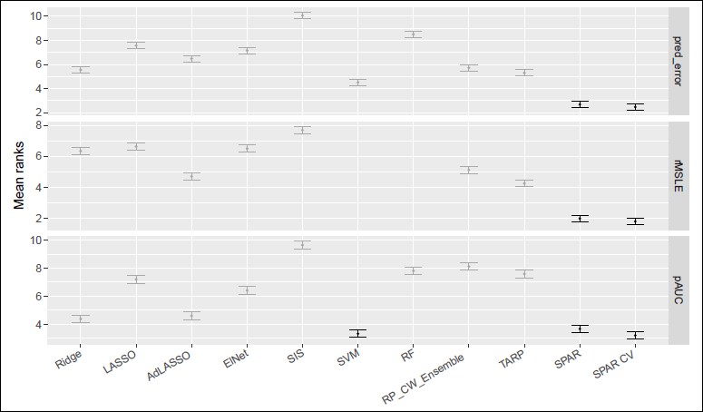
Mean ranks with 99% confidence intervals for prediction error (1 − AUC for binomial, rMSPE otherwise), link estimation (rMSLE), and variable ranking (pAUC) across all settings and nrep = 100. Methods not significantly worse than the best are shown in black.
Mean ranks with 99% confidence intervals for prediction error (1 − AUC for binomial, rMSPE otherwise), link estimation (rMSLE), and variable ranking (pAUC) across all settings and nrep = 100. Methods not significantly worse than the best are shown in black.
To evaluate overall performance, we ranked methods from best (1) to worst (11) across all settings and replications, including those in the Supplementary Materials. Figure 5 shows the average ranks (with 99% confidence intervals) across all investigated settings for each of prediction (1 AUC for binomial, rMSPE for all other families), link estimation (rMSLE) and variable ranking (pAUC). Aside from SVM in variable ranking, we find that SPAR-CV and SPAR achieved the best ranks on average over all simulation scenarios for all three measures. Using the Friedman and the post-hoc Nemenyi tests for multiple comparisons (Hollander et al., 2013), we can also report that SPAR and SPAR-CV were significantly better than all other methods for prediction and link estimation and, together with SVM, they were also significantly better for variable ranking. Even if SPAR and SPAR-CV are not best in every scenario, they perform well across the board, making them especially suitable when the degree of sparsity is unknown.
Computing time
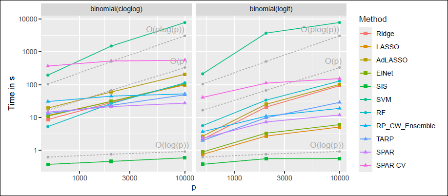
Figure 6 shows computing time for three increasing values of p for the binomial family for the medium sparsity setting with block covariance. Most methods, except RF, SVM and SIS, inherit computational efficiency from
Comparison of average computing time for increasing p, n = 200, medium sparsity and block Σ , for the binomial family.
Comparison of average computing time for increasing p, n = 200, medium sparsity and block Σ , for the binomial family.
Mean prediction metrics (with standard deviations) over 100 three-to-one train/test splits. The top three methods per dataset and metric are bolded. Note that these standard deviations do not represent formal variability estimates (e.g., confidence intervals) due to the inherent dependence across splits.
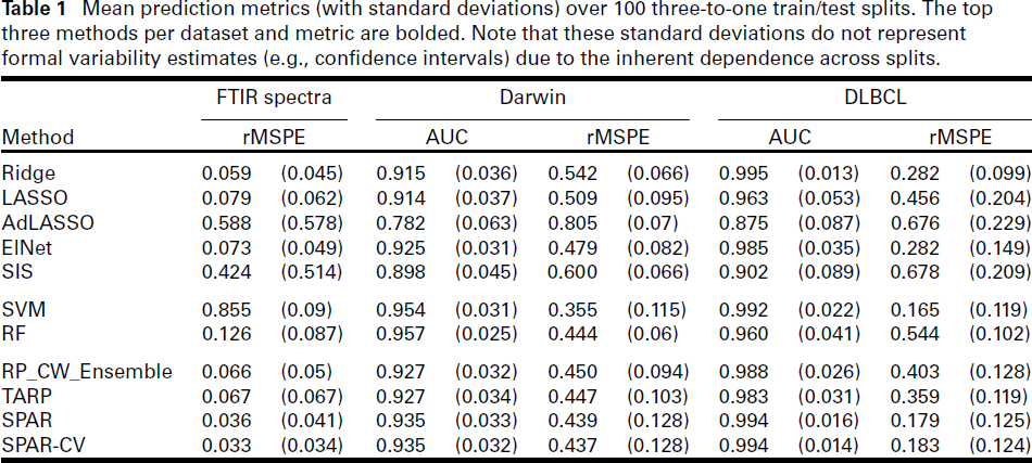
We demonstrate the proposed method on one high-dimensional dataset with a count response and two with binary responses. Results are detailed in the following sections and summarized in Table 1, which reports average prediction metrics over 100 random train/test splits (3:1 ratio). Note that while the stated standard deviations can serve as indicators for performance variation, they do not represent formal variability estimates (e.g., confidence intervals) due to the inherent dependence across splits. SPAR-CV uses deviance for cross-validation, while other methods are tuned as described in Section 3.4.
Difference FTIR spectrum for one oil sample in the tribology dataset (top) and coefficients of p = 1 814 wavenumbers estimated by SPAR-CV in each of M = 50 marginal models (bottom). Marked intervals represent non-informative variables.
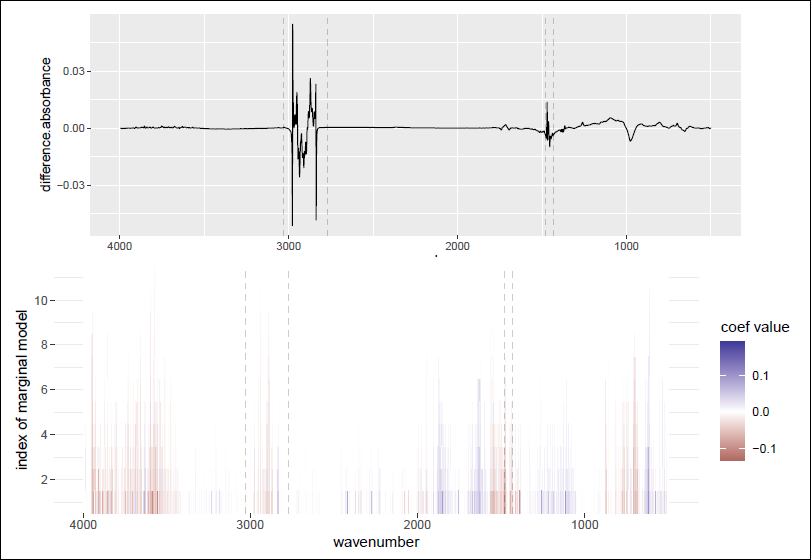
Difference FTIR spectrum for one oil sample in the tribology dataset (top) and coefficients of p = 1 814 wavenumbers estimated by SPAR-CV in each of M = 50 marginal models (bottom). Marked intervals represent non-informative variables.
Fourier transform infrared (FTIR) spectroscopy is used in tribology to analyze changes in oil samples during use. The dataset introduced in Pfeiffer et al. (2022) comprises n = 34 automotive engine oil samples that were artificially degraded under controlled laboratory conditions. Two types of artificial alteration were applied—by heating the oil and exposing it to dried air—to mimic real-world oil degradation. For each sample, the predictor variables consist of difference FTIR spectra, calculated as the absorbance difference between fresh and degraded oil, measured at p = 1814 distinct wavenumbers. The target variable is the alteration duration in hours (as integers), which quantifies how long each sample was subjected to the degradation process.
Table 1 shows the relative MSPE for various methods. SPAR-CV was estimated using Poisson, quasipoisson and Gaussian families with log links. We only present results for the Gaussian model in Table 1, as it had the best predictive performance (results for the other link functions are given in Table 3 in the Supplementary Materials). Moreover, SPAR-CV performed best overall, followed by ridge regression.
Figure 7 (top panel) displays the difference spectrum for one sample, highlighting intervals with high or total absorption. These regions, typically non-informative due to hydrocarbon properties, are often pre-processed or discarded from analysis. The bottom panel shows the standardized coefficients estimated by SPAR-CV across M = 50 marginal models (y-axis) for all variables (x-axis), where the coefficients for each variable are sorted by their absolute values and displayed vertically as a colour gradient. The distribution of coefficients across the marginal models indicates which wavenumbers correlate positively or negatively with longer alteration durations. Even without pre-processing, non-informative variables rarely appear in the models and have low coefficients when they do, demonstrating the reliability of the SPAR method.
Darwin Alzheimer dataset
The dataset, introduced in Cilia et al. (2022), contains a binary response for Alzheimer’s disease (AD) together with p = 450 extracted variables from 25 handwriting tests (18 features per task) for 89 AD patients and 85 healthy people (n = 174) and can be downloaded from the UC Irvine Machine Learning Repository. The dataset has been reported to contain outliers. We first screened for multivariate outliers and imputed them using the detect deviating cells algorithm of Rousseeuw and Bossche (2018) implemented in R package
Table 1 presents the area under the ROC curve (AUC) and the relative MSPE (rMSPE; scaled Brier score) as prediction metrics for the binary classification task. For all GLM-based methods (i.e., except SVMs and RFs), results are shown for the binomial family with logit link function. We also investigated the use of the complementary log–log (cloglog) link for these methods, but the observed performance is generally slightly worse and only Ridge and RP_CW_Ensemble achieved marginally better results with this link. Table 4 in the Supplementary Materials shows the results for both considered links.
SPAR and SPAR-CV performed similarly and were outperformed in AUC by both SVM and RF and in rMSPE by SVM alone. This suggests SPAR is a viable option for modelling this dataset, while offering low computational cost. SPAR-CV was, however, slower than RF. Table 6 in the Supplementary Materials shows the average computing time of all methods for all three data applications.
Figure 8 displays the estimated standardized coefficients for the p = 450 variables grouped by feature, across all marginal models. Feature blocks generally show either a positive or negative impact on the probability of AD across all 25 tasks (see online version for colour figures). For example, the probability of AD increases with the total time spent on a task (total_time). The number of pendowns (num_of_pendown, the number of times the pen hits the paper) is positively associated with the AD likelihood for the first few tasks, but negatively correlated for the remaining tasks, with a strong negative association observed for the task ’Copy the fields of a postal order’, which requires many pendowns when copying the individual fields. This may suggest that a lower number of pendowns in this task indicates failure to complete the task and thus a higher likelihood of AD.
Diffuse Large B-Cell Lymphoma (DLBCL)
This microarray dataset has been introduced in Shipp et al. (2002) and is available at the OpenML platform. It contains expression data for p = 5 469 genes of n = 77 patients diagnosed with two different types of lymphomas: Diffuse Large B-Cell Lymphoma (DLBCL) (58 cases) and follicular lymphoma (FL, 19 cases), making this a rather imbalanced dataset.
Again, Table 1 presents the AUC and rMSPE (scaled Brier score) as prediction metrics and for all methods based on GLMs, results are shown for the binomial family with logit. Due to the imbalance of the response, we also used the cloglog link function for these methods again, but only Ridge, LASSO and RP_CW_Ensemble achieved slightly better results with this link. Table 5 in the Supplementary Materials shows the results for both considered links.
Estimated coefficients for the p = 450 variables in the Darwin dataset, for each of the M = 50 marginal models in the SPAR-CV algorithm.
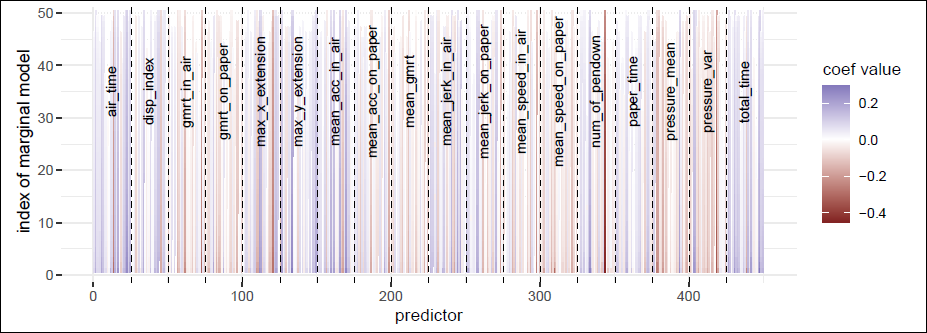
Estimated coefficients for the p = 450 variables in the Darwin dataset, for each of the M = 50 marginal models in the SPAR-CV algorithm.
On this very high-dimensional dataset, SPAR and SPAR-CV perform very well, being slightly outperformed only by SVM in terms of rMSPE and by ridge in terms of AUC.
In this article, we propose a novel data-driven random projection method to be employed in high-dimensional GLMs, which efficiently reduces the dimensionality of the problem while preserving essential information between the response and the (possibly correlated) predictors. We achieve this by using ridge-type estimates of the regression coefficients to construct the random projection matrix, which should approximately recover the true regression coefficients. These coefficients can also be employed for variable screening, which can be used before random projection to further reduce the dimensionality of the problem.
A critical aspect of the proposed method is the selection of the penalty term for the ridge-type estimator. The penalty should generally be small to avoid over-regularization. However, determining the optimal size of the penalty has proven to be a non-trivial task. For linear regression, a ridge estimator with penalty converging to zero has shown good properties (Wang and Leng, 2016; Parzer et al., 2025). In this article, we derive the analytical formula for such an estimator in GLMs with canonical links and find that this estimator leads to lower predictive performance for non-Gaussian families, likely due to overfitting. More generally, there is no one-size-fits-all penalty value for all families. Instead, we advocate for a data-driven approach by decreasing the penalty value as long as the improvement in a goodness-of-fit criterion (e.g., deviance) exceeds a certain threshold (e.g., 0.8 for non-Gaussian families and 0.999 for Gaussian).
Through extensive simulations, we show that integrating multiple probabilistic variable screening and projection steps into an ensemble of medium-sized GLMs can improve prediction accuracy and variable ranking, without too much computational cost. To implement this method, we adapt the SPAR algorithm from Parzer et al. (2025), ensuring that it is tailored to the specific requirements of high-dimensional GLMs and the method achieved good overall performance regarding ranks aggregated over all investigated scenarios, making it a valid choice when the true degree of sparsity is not known in practice. We note that the figures showing prediction and variable ranking metrics complement the aggregated ranks. While the metrics reflect performance across all replications and are influenced by data randomness, the ranks highlight consistent performance differences per replication, even if subtle. At the cost of higher computation time, which still scales well with p, the method can, to some degree, benefit from cross-validation, most notably in terms of ranking the variables based on their relevance. Even with the extensive simulation study trying to cover the most common settings, it is not certain whether the obtained results will always be generalizable to any other data-generating process encountered in practice. Final, the proposed method achieved a strong prediction performance while retaining interpretability on three real datasets, supporting the simulation results.
A potential extension includes adapting the method to multivariate GLMs (e.g., multinomial) and multivariate responses (e.g., multivariate linear regression). A key extension in this direction would be designing a data-driven random projection that can preserve the multivariate structure in the data while also being straightforward and fast to compute. Additionally, ways of incorporating non-linearities in the random projection could be explored.
Footnotes
Acknowledgement
The authors acknowledge TU Wien Bibliothek for financial support through its Open Access Funding Programme.
Declaration of Conflicting Interests
The authors declared no potential conflicts of interest with respect to the research, authorship and/or publication of this article.
Funding
The authors disclosed receipt of the following financial support for the research, authorship and/or publication of this article: Roman Parzer and Laura Vana-Gür acknowledge funding from the Austrian Science Fund (FWF) for the project ‘High-dimensional statistical learning: New methods to advance economic and sustainability policies’ (ZK 35).
Supplementary materials
References
Supplementary Material
Please find the following supplemental material available below.
For Open Access articles published under a Creative Commons License, all supplemental material carries the same license as the article it is associated with.
For non-Open Access articles published, all supplemental material carries a non-exclusive license, and permission requests for re-use of supplemental material or any part of supplemental material shall be sent directly to the copyright owner as specified in the copyright notice associated with the article.