
Abstract
Ordinal data are quite common in applied statistics. Although some model selection and regularization techniques for categorical predictors and ordinal response models have been developed over the past few years, less work has been done concerning ordinal-on-ordinal regression. Motivated by a consumer test and a survey on the willingness to pay for luxury food products consisting of Likert-type items, we propose a strategy for smoothing and selecting ordinally scaled predictors in the cumulative logit model. First, the group lasso is modified by the use of difference penalties on neighbouring dummy coefficients, thus taking into account the predictors’ ordinal structure. Second, a fused lasso-type penalty is presented for the fusion of predictor categories and factor selection. The performance of both approaches is evaluated in simulation studies and on real-world data.
Keywords
Introduction
Ordered categorical variables arise commonly in regression modelling. Still, proper treatment of the underlying scale level and appropriate statistical modelling is an issue of discussion. In many applications, particularly, the nature of ordinal predictors such as rating scales is neglected and a classical linear model is fit instead, thus assuming a metric scale level (Tutz and Gertheiss, 2014). On the other hand, statistics textbooks often transform ordinal covariates into dummy variables, thus using the variables’ nominal scale level only. Ignoring that categories are ordered implies, however, that we do not make full use of all the information contained in the data. Sometimes, when using dummy-coded ordinal predictors, monotonicity in the corresponding regression parameters is assumed to exploit the categories’ ordering (compare, for example, Young et al., 1976; Linting et al., 2007; Rufibach, 2010), which is also known under the name ‘isotonic regression’ (Barlow et al., 1972), but the assumption of monotonicity is not always plausible (Linting et al., 2007). If the dependent variable is ordinal, ordered response models as treated in most advanced textbooks on statistical modelling (e.g., Fahrmeir et al., 2013) can be used. These models are typically recommended in the statistics literature but far less used in applications; compare, for example Christensen and Brockhoff (2013). Liddell and Kruschke (2018), for instance, demonstrated that applying metric models to ordinal data can lead to significant errors, such as Type I and Type II errors and argued for the use of ordered-probit models to ensure more accurate and reliable analyses. Although modelling of ordinal response variables has been well investigated, ordinal-on-ordinal regression is hardly mentioned. A comprehensive overview of statistical models for ordinal cross-sectional data is provided by Bartolucci et al. (2015), who offer a unified framework for analyzing such data using R and Stata. To investigate the relationship between two ordinal variables, basically, any statistical tool designed for analyzing the relationship between two categorical variables arranged in a contingency table could be used. Those tools include so-called association models. For instance, the row-column (RC) model (Goodman, 1979) is a type of association model that allows us to study the interaction between the row and column categories. Such models are particularly useful in understanding how different categories of one variable are associated with the categories of another variable. However, when the number of covariates and/or the number of levels per variable becomes large, RC models are no longer practically manageable. In this work, we hence focus on ordinal regression models to analyze the effects of a set of ordinal explanatory variables on an ordinal response variable. To give an example of such a setting, let us consider a survey on luxury food (Hartmann et al., 2016, 2017), which will be the primary case study here. This survey collected data on various items measured on a five-point Likert-type scale. The primary goal of the original study was to segment German consumers based on their perceived dimensions of luxury food and the shift of consumer consumption motives toward indulgence, quality and sustainability. In what follows, we will focus on a regression problem where the response variable is the willingness to pay for luxury food products, which is also evaluated on an ordinal five-point scale. The set of predictors considered contains 43 ordinally scaled statements (items) on eating habits, shopping places and habits, the importance of price, eating style and the subjective definition of luxury food. In high-dimensional settings such as this, however, with ordinal data both on the left and right-hand side of the regression, the full regression model, such as a cumulative logit model, is often hard to fit by common maximum likelihood. Penalty-based regularization has been shown to be a viable means to handle such situations and various regularization techniques have been proposed for regression models with categorical variables over the last two decades. Meier et al. (2008), for instance, used the group lasso penalty (Yuan and Lin, 2006) for factor selection in logistic regression. Tutz and Gertheiss (2014, 2016) proposed methods for the selection of ordinally scaled independent variables in the classical linear, the logistic and the log-linear (Poisson) models. Regularized ordinal regression has been considered by Archer and Williams (2012) and Wurm et al. (2021) using a lasso-type (Tibshirani, 1996) and elastic net (Zou and Hastie, 2005) penalty, respectively.
The limitation of the penalty approaches above, however, is that they assume either the response or the predictors to be of metric scale or binary. In this article, we propose a penalty-based strategy for model selection with ordinally scaled covariates and smoothing across covariate levels in ordinal regression, specifically, the cumulative logit model. For doing so, the original group lasso is modified by the use of a difference penalty on neighbouring dummy coefficients, thus taking into account their ordinal structure. As an alternative, the use of a fused lasso-type penalty (Tibshirani et al., 2005) will be discussed.
The remainder of the article is organized as follows. Section 2 introduces two motivating data examples on food products and the corresponding modelling framework. In Section 3, we will describe in detail the two penalty methods for ordinal predictors mentioned above. Some illustrative simulation studies in Section 4 examine the quality of the proposed methodology. In Section 5, the proposed methods are applied to data from a consumer test and the study on luxury food expenditure. In Section 6, we conclude with a summary and discussion. All computations were done using the statistical programme R (R Core Team, 2021). The proposed methods are implemented in the open-source R add-on package ordPens (Gertheiss and Hoshiyar, 2023) available on CRAN and Github (
Data examples and modelling framework
Two case studies
Perception and acceptance of boar-tainted meat
For illustrative purposes, we first consider a consumer test about the perception and acceptance of boiled sausages from strongly boar-tainted meat, conducted by the Department of Animal Sciences, University of Göttingen (Meier-Dinkel et al., 2016). Due to the European call for alternatives to surgical castration of male piglets, as this practice was proven to be cruel (European Commission, 2010, 2019), there is rising interest in the production and processing of boar meat. However, there is a disadvantageous risk that off-flavors occur, the so-called boar taint, which is to be dealt with. An effort is being put into improving the processing of tainted raw material in a sustainable way with the primary aim of making it ‘fit for human consumption’. Specifically, one challenge lies in masking the undesirable odor—and the associated flavor—by combining spices, herbs and aromas and developing meat products that are palatable and accepted by consumers. The study at hand examined six sausages of different types (raw smoked-fermented or boiled emulsion-type sausages) with varying proportions of tainted raw material (50%, 100%, plus a control product without tainted material). A total of 120 participants were recruited to consume and evaluate the products with regard to different features; see Meier-Dinkel et al. (2016) for details on the recruited consumer sample. For illustrational purposes, we focus on boiled sausages here with a proportion of 50% tainted boar meat (product six). In order to process highly tainted meat sustainably, we aim to detect the relevant factors for the consumers’ overall liking. The six ordinal predictors considered ‘expected liking’, ‘appearance’, ‘odour’, ‘flavour’, ‘texture’, ‘aftertaste’ and the ordinal response ‘overall liking’ are measured on a nine-point scale (1 = ‘dislike extremely’ to 9 = ‘like extremely’). The data is summarised through barplots for selected variables in Figure 1 (top). Using a regression model, the effect of the ordinal covariates on the ordinal factor overall liking is to be investigated.
Consumers’ willingness to pay for luxury food
As a second and main case study, we consider the before-mentioned survey concerning, among other things, the consumers’ willingness to pay for ‘luxury food’ (Hartmann et al., 2016, 2017). The data was collected by a commercial panel provider and is representative of the German population with respect to age, gender and education (see Hartmann et al., 2016, 2017, for details). The part of the dataset we examine consists of 821 observations of 44 Likert-type items on personal luxury food definitions, eating and shopping habits, diet styles and food price sensitivities. One such item is, for example, ‘I associate a high price in food with particularly good quality’, with coding scheme −2 = ‘strongly disagree’, …, +2 = ‘fully agree’. The coding scheme of the remaining items is similar and given in Table C3 in the online supplements. Our response of interest is whether participants would be willing to pay a higher price for a food product that they associate with luxury, measured again on the ordinal −2 to +2 scale. The subset of the data that is analyzed here has been made publicly available at
Illustration of the sensory data. Top: frequency distribution for the covariates with levels 1 = ‘dislike extremely’ to 9 = ‘like extremely’, segmented by frequencies of response y (‘overall liking’), with colors corresponding to response categories 1 = ‘dislike extremely’ to 9 = ‘like extremely’ (see top left). Bottom: polr estimates of the regression coefficients as functions of class labels for the sensory data from Section 2.1.1. The estimated thresholds are: −34.22, −1.20, 4.84, 7.32, 8.86, 11.29, 15.75 and 21.98.
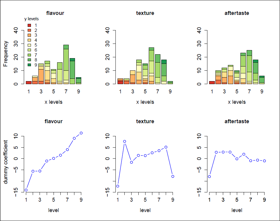
Illustration of the sensory data. Top: frequency distribution for the covariates with levels 1 = ‘dislike extremely’ to 9 = ‘like extremely’, segmented by frequencies of response y (‘overall liking’), with colors corresponding to response categories 1 = ‘dislike extremely’ to 9 = ‘like extremely’ (see top left). Bottom: polr estimates of the regression coefficients as functions of class labels for the sensory data from Section 2.1.1. The estimated thresholds are: −34.22, −1.20, 4.84, 7.32, 8.86, 11.29, 15.75 and 21.98.
The cumulative model (McCullagh, 1980) is probably the most popular regression model for ordinal response variables; compare, for example, Agresti (2010, 2013), Fahrmeir and Tutz (2001), Fahrmeir et al. (2013), Tutz (2022). It can be motivated such that the observable response variable y ∈ {1, …, c} is a categorized version of a latent continuous variable u. The link between the response variable yi (i.e., y for subject i = 1, …, n) and the corresponding latent variable ui is then defined by the threshold mechanism
With ordinal covariates, without loss of generality, each
where vector
Groupwise selection and smoothing
With categorical predictors included in the model, resulting in a large (potentially enormous) number of parameters to be estimated, typically, two challenges arise. The first step is to decide on the variables to include in the regression model. Second, we have to decide which categories within one categorical predictor should be distinguished. Furthermore, if maximizing the likelihood using (2.1), only the nominal scale level of the predictor variables is used. As already discussed by Tutz and Gertheiss (2014, 2016) for other types of regression models (namely, models with numerical, one-dimensional response), it can be beneficial to use special penalties to incorporate the predictors’ ordinal scale level. In particular, penalizing differences between coefficients that belong to adjacent categories in combination with a group lasso as done by Gertheiss et al. (2011) seems promising. The rationale behind this approach is as follows. If the levels of a categorical predictor are ordered, it may be assumed that the (expected) response does not change drastically but rather smoothly between neighbouring predictor categories. For simulation studies showing that this method is highly competitive in the classical linear model both in terms of variable selection and estimation accuracy, see Tutz and Gertheiss (2014) and Gertheiss and Tutz (2023). To implement the approach in the cumulative logit model, we will extend the logistic group lasso estimator for binary responses (Meier et al., 2008) to the class of cumulative logit models. This type of estimator is given by the minimizer of the function
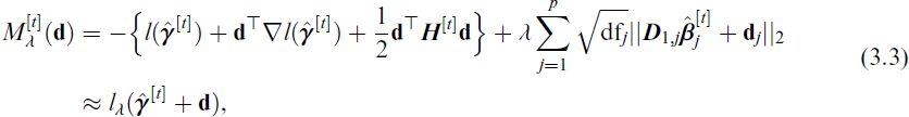
where l(θ, β) is the log-likelihood of the cumulative logistic distributionin (2.2); vectors θ and β collect all thresholds θ1, …, θc−1 and subvectors β1, …, βp, respectively. In order to take into account the ordinal structure of the predictors, we modify the usual L2-norm of the group lasso by the first-order difference penalty functions
with kj being the number of levels of the jth covariate and
To find the final solution, we can utilize the block coordinate gradient descent method of Tseng and Yun (2009), as described in Meier et al. (2008). Namely, it combines a quadratic approximation of the log-likelihood with an additional line search. Based on the coordinate descent algorithm, the R package grplasso (Meier, 2020) provides (standard) group lasso estimation for the Poisson, the logistic and the classical linear models. For penalized ordinal-on-ordinal regression in terms of a cumulative logit model with ordinal predictors and corresponding ordinal smoothing penalty (3.2) some modifications have to be made. Using a second-order Taylor series expansion at
with

the minimizer of
The strength of penalization is controlled by the parameter λ. With λ = 0, unpenalized maximum likelihood estimates for categorical variables as described in Section 2.2 are obtained. If λ → ∞ one obtains the extreme case that coefficients that belong to the same predictor are estimated to be equal, which means that the corresponding predictor has no effect on the response. In fact, with any of the restrictions (reference category set to zero or effect coding), all parameters except for thresholds are estimated to be zero if λ → ∞. Further, note that penalized estimates as proposed here are invariant against the concrete choice of the restrictions because the values of both the likelihood and penalty at (3.2) do not depend on the restriction chosen. Note that we do not penalize thresholds θr.
If a variable is selected by the smoothed group lasso (3.2), all coefficients belonging to that selected covariate are estimated as differing (at least slightly). However, it might be useful to fuse certain categories. Fusion of dummy coefficients of ordinal predictors has already been discussed by Tutz and Gertheiss (2014, 2016) for regression models with numerical, one-dimensional response; namely, the classical linear model and a generalized linear model with binary or count data (Poisson) response. Having data such as those described in Section 2.1 in mind, we extend this previous work to the multivariate case of multi-categorical, ordinal response models; specifically, the framework of the cumulative logit model. Fusion is done by a fused lasso-type penalty (Tibshirani et al., 2005) using the L1-norm on adjacent categories. That is, adjacent categories may end up with exactly the same coefficient values and one obtains clusters of categories. The idea is to maximize lλ(θ, β) from (3.1) above with
Using the L1-norm for neighbouring categories encourages that adjacent parameters are set exactly equal rather than just being close (as done by penalty (3.2)). Penalty (3.5) thus has the effect that neighbouring categories may be fused (namely, if they have the same β values). The fused lasso also enables the selection of predictors: A predictor is excluded if all its categories are combined into one cluster. As already pointed out in Section 3.1 above, any of the restrictions considered here then means that all parameters belonging to the respective predictor are set to zero. As before, penalty (3.5) is invariant against the concrete choice of restriction. After reparametrization, our fused lasso variant can be fit using existing software for the lasso. Technical details can be found in Appendix A.3.
An alternative to the one-step, penalized likelihood methods presented in this article would be to use regularization for model selection only (i.e., identification of the relevant covariates and relevant differences between predictor levels). Afterward, the final model would be re-fit on the reduced and collapsed data through common, unpenalized maximum likelihood. Such an approach was, for example, used in Gertheiss and Tutz (2010) and is also known under the name ‘post-lasso’ (Belloni et al., 2012; Belloni and Chernozhukov, 2013).
Cross validation
In the definitions and algorithms above, the penalty parameter λ was fixed at some specific value. However, the choice of an optimal value for λ should be made using the data at hand. A common strategy in penalized regression is K-fold cross-validation as described in many textbooks, for example, Hastie et al. (2009). As a measure of performance, we calculate the Brier score (Brier, 1950)
Stability selection
The previous section described a potential process for selecting the regularization parameter, with the selection of this parameter also implying the particular set of features being selected. Particularly for high-dimensional data, cross-validation techniques can be quite challenging as cross-validated choices may include too many variables (Leng et al., 2006; Meinshausen and Bühlmann, 2006). If we are mainly interested in feature selection, we can alternatively apply stability selection as suggested by Meinshausen and Bühlmann (2010), a promising subsampling strategy combined with high-dimensional variable selection. In general, instead of selecting/fitting one model, the data are perturbed or subsampled many times and we choose those variables that occur in a large fraction of runs. Specifically, for the jth variable, the estimated probability
Numerical experiments
Study design
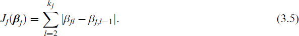
Before applying the presented methodology to the real-world data in Section 5, we carry out a simulation study to investigate the properties of the proposed ordinal-on-ordinal selection approach using penalties (3.2) and (3.5). We generate p = 50 ordinally scaled covariates X1, …, X50, including 38 noise variables as follows: X1, …, X4 have non-monotone effects, X5, …, X8 are monotone but non-linear and the effect of X9, …, X12 is linear across categories. The remaining 38 predictors are irrelevant, that is, with zero effects. Each predictor is assumed to have the same number of levels, either five or nine, depending on the concrete setting considered. Factor levels are then randomly drawn from {1, …, 5} or {1, …, 9}, respectively. The (true) covariate effects are shown in Figure 2. Using those predictors, we construct the ordinal response (with five levels) through the cumulative logit model with linear predictor (2.1) and thresholds θ = (5.5, 6.5, 7.5, 8.5)⊤ and consider three different sample sizes n = 200, 500 and 1 000.
True effects of influential predictors in the simulation study. (a) five levels without fused effects; (b) nine levels without fused effects; (c) five levels with fused effects; (d) nine levels with fused effects.
True effects of influential predictors in the simulation study. (a) five levels without fused effects; (b) nine levels without fused effects; (c) five levels with fused effects; (d) nine levels with fused effects.
We assign ranks to the predictor items according to the order of non-zero ordinal group lasso coefficients in the coefficient path and call this ordinal rank selection (ORS). Similarly, we proceed with the non-zero ordinal fused lasso coefficients in the corresponding coefficient path and call this ordinal rank fusion (ORF). We compare these two approaches to two competitors: (a) the standard POM fit by polr and combined with AIC-based forward stepwise selection where the ordinal covariate is treated as nominal, that is, it is dummy-coded without any penalization and (b) treating the predictor as numeric and employing ordinalNet with a standard lasso penalty for selection. Note that the usual ordinalNet function offers no (nominal/ordinal) group lasso option. Thus, the selection of ordinal responses is only accessible if we ignore the categorical nature of the covariates. The entire data generation and estimation/selection process was repeated 100 times. The results are discussed below.
Variable selection
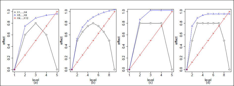
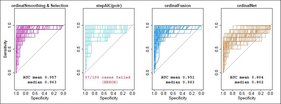
To evaluate the methods’ performance in terms of variable selection, we construct the Receiver Operating Characteristic (ROC) (Fawcett, 2006) by varying selection thresholds λ (for ORS, ORF and ordinalNet) and calculate the area under this curve (AUC) in each iteration. Briefly, we evaluate the estimated models as a binary classification task, where covariates are predicted to be present or absent. For polr, the order of variables entering the (forward) stepwise selected model is used for ranking. Variables that were not selected at all are randomly coerced to the back. We only discuss the results of scenario (a) from Figure 2 in detail here, where true effects contain unfused effects of five levels. Due to a lack of space, we refer to the online supplementary material for the other settings’ results. Figures 3 and 4 show the performance in terms of the ROC as obtained with varying λ values, for n = 200 and n = 500, respectively. Additionally, the mean and median AUC for each method are given. The results for the remaining scenarios can be found in the online supplementary material (Figures C1–C12). Even with the relatively large sample size of 500, polr failed in 37 of the datasets (zero cases with n = 1 000, but all cases with n = 200). This result is in line with the issues that we observed with the standard POM for the boar-taint data in Section 2.2. The mean and median AUC over the 63 successful runs with n = 500 were 0.908 and 0.919, respectively. By contrast, the ordinal penalties work very well and both account for the ordinal-on-ordinal nature. In general, the choice between penalties (3.2) and (3.5) depends on the concrete application and personal preferences. While both enforce the selection of predictors, ORS yields smooth effects of predictors, whereas ORF yields parameter estimates that tend to be flat over some neighbouring categories, which represents a specific form of smoothness, too. The classical ordinalNet approach, however, is inferior for model selection since it offers no group lasso option for categorical or ordinal predictors. With n = 1 000 (not shown here), all methods—except for classical lasso—work (almost) equally well in scenarios (a) and (c). In scenarios (b) and (d), that is, with predictors having nine levels each, polr performs even worse than Figure 4, as estimation now fails in all cases with n = 500. Even with n = 1 000, polr is inferior to penalized selection and fusion in the nine predictor level setting (compare the online appendix for details, Figures C4–6 and C10–12).
ROC curves when using ORS, polr, ORF or ordinalNet for finding the relevant variables in terms of a binary ‘classification’ task with n = 200 according to simulation setting (a) from Figure 2 (five levels without fused effects).
ROC curves when using ORS, polr, ORF or ordinalNet for finding the relevant variables in terms of a binary ‘classification’ task with n = 200 according to simulation setting (a) from Figure 2 (five levels without fused effects).
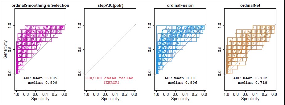
ROC curves when using ORS, polr, ORF or ordinalNet for finding the relevant variables in terms of a binary ‘classification’ task with n = 500 according to simulation setting (a) from Figure 2 (five levels without fused effects).
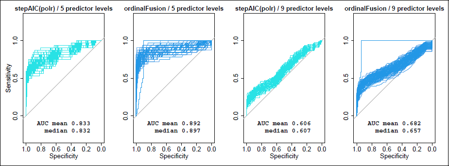
ROC curves when using polr or ordinalFusion concerning the identification of relevant differences (i.e., fusion) of dummy coefficients for n = 1 000. Left: five levels with fused effects; right: nine levels with fused effects; that is, setting (c) and (d) from Figure 2, respectively.
To gain more insights into the different behaviours of the competing methods, we tested whether differences in AUC values are statistically significant. Table C2 in the online appendix presents the p-values of the corresponding (paired) t-tests, Table C3 shows fractions of p-values ≤ .05 of the DeLong test (DeLong et al., 1988). It is seen that the performance of the proposed penalties ORS and ORF does not significantly differ in most cases. Graphical comparisons of AUC values confirm these findings (Figures C13 and C14 in the online appendix). It is a positive result that the ROC and AUC of the considered fusion and smoothing/selection penalty are very similar, indicating that the fusion penalty performs well for variable selection purposes, too.
The results discussed so far concern the identification of relevant predictors. In scenarios (c) and (d), however, we are also interested in comparing the performance regarding the identification of relevant differences (i.e., fusion between adjacent dummy coefficients). For this purpose, we consider estimates using penalty (3.5). Figure 5 shows the performance in terms of ROC as obtained with varying λ and n = 1 000. In addition, we run stepAIC(polr) as a competing model, but on the re-coded design matrix (Walter et al., 1987), thus selecting (presumably relevant) differences between neighbouring categories. The run time of polr increases dramatically as contrasts of factor levels now enter and leave the model in each step separately. Figure C15 in the supplementary material illustrates the false positive/negative rates (FPR/FNR). With five underlying levels (scenario (c)) and n = 500, stepAIC(polr) only converged in 23 cases and, not surprisingly, in zero cases for n = 200. This is why we only present results for the largest sample size n = 1 000 in Figure 5. With nine underlying levels (scenario (d)), estimation with polr failed in all cases with n = 200 and n = 500. The poorer performance compared to variable selection (see also Figures C9 and C12, online appendix) is due to the fact that with selection, it is sufficient for a correct result (in terms of a ‘true positive’) if at least one contrast was selected. For identification of the relevant differences, however, all contrasts of neighbouring categories are checked individually. The finding that AUC-values in Figure 5 tend to be lower in the nine-levels case (right) than in the five-levels case (left) can at least partly be explained by the fact that the former model has much more parameters and that contrasts that were not selected at all are coerced to the back in a random order before drawing or calculating the ROC/AUC. However, the fusion penalty still works better than polr with stepwise selection.
Application to case studies
Perception and acceptance of boar-tainted meat
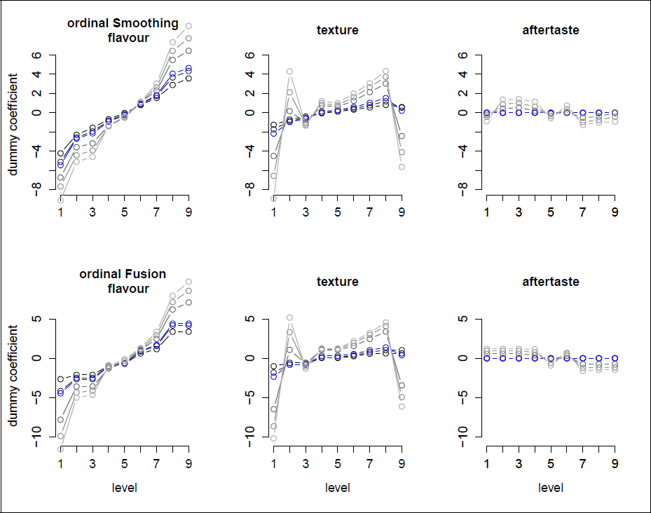
To illustrate the application of penalized ordinal-on-ordinal regression in practice, we first consider the boar-taint example from Section 2.1.1. The study aimed to identify important factors for consumer acceptance of boar-tainted meat. Determining the most important predictors of overall liking would be of great interest for the development of palatable products. Figure 6 (top) shows the resulting parameter estimates for the selected covariates and different values of tuning parameter λ when applying the proposed groupwise selection and smoothing method. Results of the remaining variables can be found in Appendix D. It is seen that for smaller λ (light gray), the estimates are more wiggly (and more extreme) and become more and more smoothed out/shrunken as λ increases. It is also seen that, at some point, the entire group of dummy coefficients belonging to one variable is set to zero, which means that the corresponding variable is excluded from the model. Figure 6 (bottom) shows the fitted coefficients when the fusion penalty (3.5) is employed. It is seen that some of the categories are fused, indicating that, at least for some variables, fewer rating categories would be sufficient to model the effect on overall liking. In general, the overall liking increases with the liking level of the covariates, with flavour apparently having the largest effect, followed by appearance and texture. On the other hand, the expected liking, the odour and the aftertaste seem to be much less relevant. The obvious consequence of these findings is that, to make meat from entire male pigs more attractive to consumers, the producers (of processed meat) should try to make their products look and, most importantly, taste better, for example, using spices masking the boar taint (Mörlein et al., 2019).
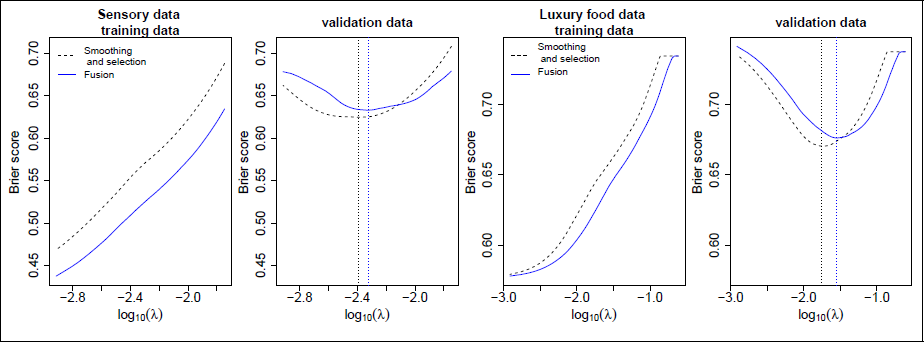
The predictive performance according to five-fold cross-validation on the boar-taint data for both the smooth group and fused lasso as a function of λ is given in Figure 7 (left panels). On the training data, this function is monotonically increasing in λ, as with smaller λ, more emphasis is put on the data. On the validation data, however, we see that the unpenalized POM (see λ → 0, i.e., log10(λ) → −∞) is worse than smoothed selection or fusion. Cross-validation results thus indicate that predictive performance can be enhanced using the suggested penalized method(s). Performance improves on the validation data up to a certain λ value and deteriorates from there. Note that the shift in the curves for the training data is not to be understood in the y-direction but in the x-direction. This is because the penalties are not directly comparable with each other. The optimal smoothing parameter, as determined on the validation set(s), is indicated by the dotted lines in Figure 7. Based on those results, we can use the optimal λ (where the Brier score on the validation data reaches its minimum) to fit the final model. The resulting estimates are marked in blue in Figure 6. The stability paths for the selection penalty (3.2) and the fusion penalty (3.5), indicating the order of relevance of the predictors according to stability selection are found in the supplementary material (Figure C27).
Estimation results for the sensory data from Section 2.1.1. Top: Cumulative group lasso estimates of the regression coefficients as functions of class labels (λ ∈ {10, 5, 1, 0.5, 0.25}/n). Light grey indicates smaller λ. Blue lines correspond to cross-validated/optimal λ = 3.5/n. Bottom: Cumulative fused lasso estimates of the regression coefficients as functions of class labels (λ ∈ {10, 5, 1, 0.5, 0.25}/n). Light grey indicates smaller λ. Blue lines correspond to cross-validated/optimal λ = 4/n.
Estimation results for the sensory data from Section 2.1.1. Top: Cumulative group lasso estimates of the regression coefficients as functions of class labels (λ ∈ {10, 5, 1, 0.5, 0.25}/n). Light grey indicates smaller λ. Blue lines correspond to cross-validated/optimal λ = 3.5/n. Bottom: Cumulative fused lasso estimates of the regression coefficients as functions of class labels (λ ∈ {10, 5, 1, 0.5, 0.25}/n). Light grey indicates smaller λ. Blue lines correspond to cross-validated/optimal λ = 4/n.
We use penalties (3.2) and (3.5) when modelling the luxury food data as described in the Introduction and Section 2.1.2. The descriptive statistics on the data analyzed can be found in the online supplementary material, covering, among other things, a description of the items along with observed frequencies (Table C4 and Figure C16) and the correlation plot (Figure C22). The code used for the presented case study is given in the vignette of our R package ordPens (
Brier score (averaged over all folds) with ordinal smooth selection penalty (black dashed) and with ordinal fusion penalty (blue solid) for the sensory data from Section 2.1.1 (left panels) and for the luxury food data from Section 2.1.2 (right panels).
Brier score (averaged over all folds) with ordinal smooth selection penalty (black dashed) and with ordinal fusion penalty (blue solid) for the sensory data from Section 2.1.1 (left panels) and for the luxury food data from Section 2.1.2 (right panels).
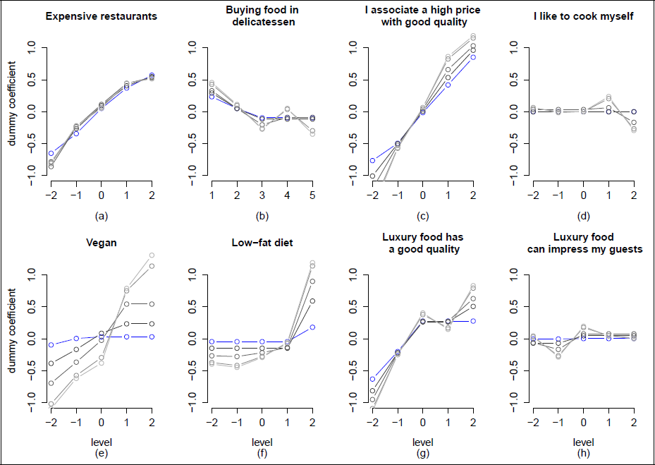
Figure 8 illustrates the resulting parameter estimates for selected covariates and different values of tuning parameter λ when applying the ordinal group lasso. Figure 9 shows the corresponding results for the ordinal fused lasso. Similarly to the boar data example, the estimates are more wiggly for smaller λ (light grey) but become smoother and shrunken as λ increases. Especially, the willingness to pay tends to increase among people who (a) eat out frequently in expensive restaurants, (c) associate a high price with good quality and (g) associate luxury with high quality. Our findings thus contribute to the literature on food and luxury by providing additional information about the kind of consumer who may be willing to pay a higher price for ‘luxury food’. For some items, for example, ‘I like to cook myself’ and ‘Luxury food can impress my guests,’ however, we observe rather flat effects that quickly go to zero as soon as λ increases (compare the most right panel in Figure 9), indicating that those items and, hence, corresponding attitudes, provide only limited information regarding the respondent’s willingness to pay for luxury food. As a consequence, for example, a producer of luxury food, it might not be worth targeting consumers (e.g., through a TV ad where a party host impresses the guests by serving luxury food) who primarily want to ‘show off’ (compare Figure 9, bottom right). Instead of that, the food producer should rather emphasize the food’s high quality (compare Figure 9, third panel). From a more general perspective, Wiedmann et al. (2009) and Shirai (2015) already discussed the perceived association of luxury, quality and price. Alfnes and Sharma (2010) and Parsa et al. (2017) specifically considered customers in restaurants, highlighted price as a perceived positive indicator for the quality of food and investigated ways to increase the willingness to pay, respectively. An overview of the estimated effects of all items considered in our study is given in the supplementary material (Figures C17–C21). Since the effects of penalties (3.2) and (3.5) are quite similar, only the results of the fused lasso are presented there.
Cumulative group lasso estimates of the regression coefficients as functions of class labels (λ ∈ 14.5, 10, 5, 1, 0.25/n) for the luxury food data from Section 2.1.2. Light grey indicates smaller λ. Blue lines correspond to cross-validated/optimal λ = 14.5/n.
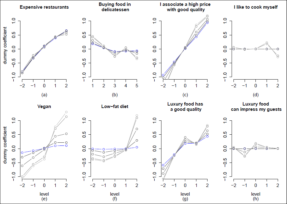
Cumulative group lasso estimates of the regression coefficients as functions of class labels (λ ∈ 14.5, 10, 5, 1, 0.25/n) for the luxury food data from Section 2.1.2. Light grey indicates smaller λ. Blue lines correspond to cross-validated/optimal λ = 14.5/n.
The (fivefold) cross-validated predictive performance in terms of the Brier Score as a function of λ is given in Figure 7 (right panels). If using the fused lasso and choosing the amount of penalty through (fivefold) cross-validation, we obtain an optimal λ around 18.5/n (marked by the dotted blue line in Figure 7). The corresponding estimates of the covariates’ effects are highlighted in blue in Figure 9. For the variable (g) ‘Luxury food has a good quality,’ for example, it is seen that the upper three categories are fused. If using the ordinal group lasso instead, the optimal (cross-validated) λ is around 14.5/n (marked by the dotted black line in Figure 7), with the resulting estimates in Figure 8 indicated by the blue lines. If choosing λ = 14.5/n to obtain a final model, 17 variables are removed and 26 variables are selected by the ordinal group lasso (with some showing very small effects, though). The most influential factors are those already shown in Figure 8: (a) Expensive restaurants, (c) associating a high price with good quality and (g) associating luxury with high quality. With the fused lasso, however, we might be more interested in detecting significant differences. To understand the fitted model’s complexity, we refer to the degrees of freedom (df). For the fused lasso, an approximation is given by the number of non-zero parameters, that is, non-zero differences of adjacent (dummy) coefficients (cf. Tibshirani et al., 2005). If using λ = 18.5/n for the ordinal fused lasso, we detect 51 relevant differences, which corresponds to about one-third compared to a total of 43 × 4 = 172 parameters in the full model.
Cumulative fused lasso estimates of the regression coefficients as functions of class labels (λ ∈ 18.5, 10, 5, 1, 0.25/n) for the luxury food data from Section 2.1.2. Light grey indicates smaller λ. Blue lines correspond to cross-validated/optimal λ = 18.5/n.
With the fusion penalty, in total 3.9 seconds elapsed when estimating the final model (i.e., using the optimal amount of penalization according to Figure 7) on a MacBook with a 2.3 GHz processor and 16 GB RAM. With the smoothing/selection penalty, 5.7 seconds elapsed. It should be noted, though, that the computation for a grid of λ values does not increase the computational time by a factor of the length of the grid compared to a single λ. This is because our algorithm sorts the provided λ in decreasing order and utilizes the results from the previous λ value for a ‘warm start’. This approach significantly reduces the computational burden when working with multiple λ values. For instance, running our ordinal group lasso algorithm (on the complete dataset) on a grid of five different λ values (as done to create Figure 8) took approximately 14.9 seconds.
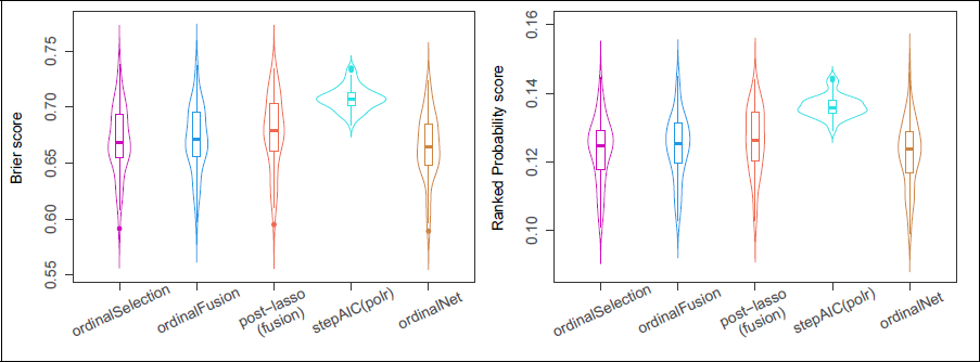
Prediction accuracy (lower values are better) in terms of the test set Brier (left) and ranked probability (right) score for 50 random splits of the luxury food data from Section 2.1.2.
Prediction accuracy (lower values are better) in terms of the test set Brier (left) and ranked probability (right) score for 50 random splits of the luxury food data from Section 2.1.2.
In order to evaluate the prediction accuracy of the models obtained using the proposed penalties (3.2) and (3.5), including ‘post-(fused) lasso’, we performed repeated random splitting of the luxury data into training and test sets. That means all regression parameters are estimated on the training data (including the choice of the tuning parameter) and then used to predict the test data. As the test set size, we choose 100 and the procedure is independently repeated 50 times. As before in the simulations studies, we compare our ordinal group and fused lasso with the ordinalNet and a common POM/AIC-based stepwise selection. Resulting violin plots are shown in Figure 10. Performance is measured in terms of the test set Brier Score (left) and ranked probability score (right). In the simulation studies in Section 4.2.1, we saw that the common POM with factor variables performed well in large samples and was superior to ordinalNet. In the simulation studies, however, we had a controlled setting with partially non-linear and even non-monotonic effects. Results on the luxury dataset are somewhat different. Although the dataset has a moderate sample size, the unpenalized POM seems to attribute too much importance to random noise in the data and, therefore, tends to overfit. The considered penalty methods, on the other hand, perform equally well, indicating that the covariates’ effects are approximated reasonably well by linear functions of the integer-valued predictor levels (as the latter is done by ordinalNet). The post-lasso does not provide any (further) benefit on this dataset.
In the present work, we proposed two ways of regularization in ordinal-on-ordinal regression. By use of tailored penalty terms, these methods effectively extract information from ordinally scaled predictors and account for ordinal response variables. In particular, an L2-difference penalty of first order for the selection of relevant factors and an L1 variant for fusion of categories were presented. These approaches are more flexible than the methods existing so far for ordinal responses in combination with ordinal predictors and allow for smoothing of covariate effects. The proposed methodology is implemented in R and publicly available on CRAN through add-on package ordPens.
To motivate and illustrate the proposed methods and to show their potential benefits, we presented two real-world examples of item-on-items regression. First, we considered a consumer test on the acceptance and perception of boar-tainted meat. The corresponding dataset consisted of seven Likert-type items with nine levels each. In summary, our presented results suggest that penalized regression works well in the cumulative logit model with ordinally scaled predictors and ordinal group or fused lasso penalty. We combined the penalty approach with stability selection to gain additional information about a variable’s probability to be included in the model, given a certain amount of penalization. Namely, if trying to predict the product’s overall liking score, the stability path revealed that the probability to be selected (within resampling) is highest for the flavour, the texture and the appearance of the meat product.
For comparison, we considered the standard POM implemented in the polr() R-function, which simply treats categorical/ordinal covariates as dummy-coded factors and offers no option for smoothing. We found that the use of polr can cause problems as (a) the employed fitting routine often fails (even for moderately dimensioned setups) and (b) often results in wiggly/implausible estimates of the (categorical) covariates’ effects. Our numerical experiments distinguished between settings involving five or nine predictor levels. In summary, polr only worked well when the sample size was large enough and (often) failed otherwise. Ordinal selection and ordinal fusion worked equally well and outperformed polr in most scenarios. Overall, performance deteriorated with an increasing number of category levels, that is, increasing model complexity. In addition, we compared our smoothing/selection and fusion penalties to the classical lasso for the cumulative logit model as implemented in ordinalNet(). This method offers no group lasso option for the selection of categorical predictors. In our numerical experiments, it was thus not particularly surprising that in terms of AUC values, standard ordinalNet with linear effects performed worst and therefore seems somewhat unsuited for ordinal-on-ordinal regression if at least some of the effects may be non-linear across factor levels or even non-monotone.
Our main interest was in a high-dimensional survey on luxury food expenditure, again consisting of Likert-type items. On the one hand, it can be assumed that in a dataset of this size, not all of the (43) items will be relevant for explaining the response, making variable selection a primary concern. On the other hand, we would like to have estimates that are rather smooth and interpretable while taking the covariates’ ordinal scale level into account. In summary, penalized (cumulative logit) regression appeared to be a sensible approach in studies of this type. For some items, we could observe that most categories were fused. For some (presumably) less relevant items, it could be seen that they reached effects equal to zero quickly as the amount of penalization increased. To obtain a final model, an appropriate penalty parameter was chosen using cross-validation. With the group lasso, eventually, about 40% of the covariates were removed from the model. With the fused lasso, we detected about one-third of the parameters to be relevant (in the sense of non-zero differences between adjacent categories).
Footnotes
Declaration of Conflicting Interests
The authors declared no potential conflicts of interest with respect to the research, authorship and/or publication of this article.
Funding
The authors disclosed receipt of the following financial support for the research, authorship and/or publication of this article: A. Hoshiyar’s and J. Gertheiss’ research was supported by Deutsche Forschungsgemeinschaft (DFG) under Grant GE2353/2-1.
Supplementary materials
References
Supplementary Material
Please find the following supplemental material available below.
For Open Access articles published under a Creative Commons License, all supplemental material carries the same license as the article it is associated with.
For non-Open Access articles published, all supplemental material carries a non-exclusive license, and permission requests for re-use of supplemental material or any part of supplemental material shall be sent directly to the copyright owner as specified in the copyright notice associated with the article.