
Abstract
A general random effects model is proposed that allows for continuous as well as discrete distributions of the responses. Responses can be unrestricted continuous, bounded continuous, binary, ordered categorical or given in the form of counts. The distribution of the responses is not restricted to exponential families, which is a severe restriction in generalized mixed models. Generalized mixed models use fixed distributions for responses, for example the Poisson distribution in count data, which has the disadvantage of not accounting for overdispersion. By using a response function and a threshold function, the proposed mixed threshold model can account for a variety of alternative distributions that often show better fits than fixed distributions used within the generalized linear model framework. A particular strength of the model is that it provides a tool for joint modelling, responses may be of different types, some can be discrete, others continuous.
Introduction
Random effects models are a strong tool to model the heterogeneity of clustered responses. By postulating the existence of unobserved latent variables, the so-called random effects, which are shared by the measurement within a cluster, correlation between the measurements within clusters is introduced. The clusters or units can refer to persons in repeated measurement trials or to larger units as, for example, schools with measurements referring to performance scores of students.
Detailed expositions of linear mixed models, which are typically used for continuous dependent variables, are found in Hsiao (1986), Lindsey (1993) and Jones (1993). Models for binary variables and counts are often discussed within the framework of generalized mixed models, see, for example, McCulloch and Searle (2001). Random effects models for ordinal dependent variables were considered by Harville and Mee (1984), Jansen (1990), Tutz and Hennevogl (1996) and Hartzel et al. (2001). Mixed model versions for continuous bounded data in the form of rates and proportions that take values in the interval (0, 1) have been considered by Qiu et al. (2008) based on the simplex model and by Bonat et al. (2015) who propagate beta distribution models. Several R packages are available to fit generalized mixed linear models, for example,
Generalized mixed models within the generalized linear model framework as well as extended approaches as the models for bounded continuous data postulate familiar fixed distributions for the responses. This is different in the approach propagated here, although there is some overlap with generalized linear models. The mixed threshold model used here gains its flexibility concerning distributional assumptions by using two components, a response function, which is a distribution function, and a threshold function that modifies the distribution. In the simplest case, by assuming a linear threshold function, the distribution of the responses follows the response function. Thus, familiar linear Gaussian response models are obtained but also linear models with quite different, possibly skewed distribution functions are available. Distributions with a restricted support, for example if responses are observed in an interval or are positive only, are obtained by using non-linear threshold functions. They are also useful when modelling discrete data, which typically are restricted to a specific range, for example, count data take only values 0, 1, … and ordered categorical responses, can be coded by 0, 1, …, k, where numbers only represent the order of values. In the case of binary and ordered categorical responses, the cumulative generalized mixed model is a special case of the proposed threshold model.
More concretely, let

where F(.) is a strictly increasing distribution function and δj(.)) is a non-decreasing measurement-specific function defined on the support S of the dependent variables, referred to as threshold function. The function δj(.) is a function to be specified whose parameters are estimated jointly with the other model parameters. In addition, it is assumed that the observations
The predictor
The term
The term
The distribution of the dependent variables is crucially determined by the choice of the distribution function F(.), also referred to as response function, and the threshold function δj(.). Specific choices yield models that are in common use in random effects modelling. Other choices widen the toolbox yielding models that show better fits than classical approaches. Threshold models have been considered before in the form of item threshold model (Tutz, 2022), which are latent trait models that aim at measurement and do not contain any covariates. In the item response model, it is assumed that the responses on a collection of items depend on the latent abilities or attitudes of persons and the difficulties of the items. Items are considered tools to measure the ability or attitude. In the random effects models considered here, the objective is quite different. The focus is on the effect of covariates on responses, random effects are used to account for the heterogeneity of respondents and covariates, and their effects are explicitly included. The role the response and the threshold functions play in modelling the response distribution will become obvious when considering specific choices.
The strengths of the modelling approach are in particular:
The model provides a common framework for different types of responses, which may be continuous or discrete. If responses are continuous, the model allows for alternative distributions that can fit much better than the typically used normal response mixed model. In particular, restrictions on the responses can be adequately modelled. Responses can be bounded, that is, restricted to an interval providing flexible alternatives to fixed distribution approaches as the beta distribution. Specific choices of the threshold functions provide alternative models for positive-valued responses. Within the model framework, discrete responses can be finite or have infinite support. In the case of binary or ordered categorical data, familiar models as the random effects version of the proportional odds model are special cases. In the case of count data, the model is an alternative to fixed distribution models as the Poisson model. The common framework allows to develop software that fits all the models that are included. The model does not assume that the form of the distribution is the same across measurement. In general, the type of the distribution can be specified measurement-specific allowing in particular for the joint modelling of discrete and continuous distributions.
In Section 2 the case of continuous responses is considered with linear and non-linear threshold functions. Section 3 is devoted to discrete data with infinite and finite support. Joint modelling, which allows for different types of responses, in particular a mixture of continuous and discrete responses, is considered in Section 4. Marginal likelihood estimation methods are given in Section 5. Several small examples are used to demonstrate the versatility of the approach. They are meant for illustration, and no in-depth investigation of effects is given.
We start with models that contain linear threshold functions. The model class comprises the classical normal response model but allows for alternative distributions. Then we consider models for restricted support, which call for non-linear threshold functions.
Linear random effects models for Gaussian data and other distributions
Let the dependent variables be continuous with support
Let F(.) denote a fixed, typically standardized, distribution function with support

where
It is seen from equation (2.1) that the means of dependent variables are simple linear functions of
The distribution of responses is easily derived since the density fij(.) of variable Yij is given by

where f(.) denotes the density linked to F(.),
A simplified version is the homogeneous MTM, in which δj does not depend on the measurement, that is,

where
A special case of the MTM is the classical linear random effects model with normally distributed dependent variables. Let F(.) denote the standardized normal distribution function and assume that dispersion homogeneity holds

where
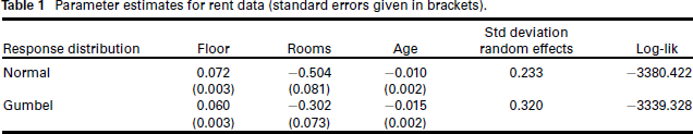
Parameter estimates for rent data (standard errors given in brackets).
The more general model with varying dispersion parameters δj is an extension of this classical model. It is more flexible and can be more appropriate, in particular when repeated measurements on a unit are time-dependent and the variance changes over time.
Within the MTM framework there is no need to assume that dependent variables are normally distributed. Any strictly monotone distribution function F(.) can be used in the model. With linear threshold function δj(.) one obtains a linear form of the expectation and simple terms for the variance. In particular, skewed distribution can be used. This extends the usual normal distribution approach to modelling clustered data to a wider class of models with a simple link between covariates and measurements.
Rent data
For illustration we use the Munich rent index data. The variables are rent (monthly rent in Euros), floor (floor space), rooms (number of rooms) and age in years. There are 25 districts (residential areas) which have an effect on rents and are modelled as random effects. For an extensive description of the rent data, see Fahrmeir et al. (2011). The rent is the dependent variable. Floor space, number of rooms and age are explanatory variables, which are assumed to have global effects, that is,
Monthly rents tend to have a right-skewed distribution since there are typically some houses that are much more expensive than the average house. Thus, the normal distribution might not be the best choice for modelling this kind of data. A candidate for a right right-skewed distribution is the Gumbel distribution
In many applications the dependent variable can take only positive values, for example if responses are response times. Although often used, the assumption of a normal distribution or any other distribution with support
In the MTM the support of the dependent variable can be restricted by using an appropriate threshold function δj(.). If the difficulty function is chosen such that 
Threshold functions of this type combine linearity with a transformation function. The general form of threshold functions of this type, which are used throughout the paper, is

where g(.) is a non-decreasing function. Threshold functions of this form are simply named after the transformation function g(.).
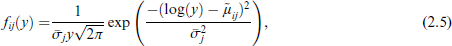
If the threshold function is logarithmic a familiar distribution is found if F(.) is chosen as the standard normal distribution function. Then, one can derive that the density of yij denoted by fij(.) is given by
where
Sleep data
In a sleep deprivation study, the average reaction time per day for subjects has been measured (data set sleepstudy from package
Instead of using a normal distribution model with linear effect of days a threshold model with normal response function and logarithmic threshold function is used. In the model

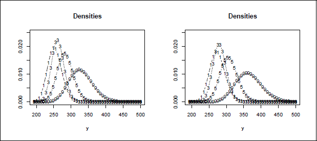
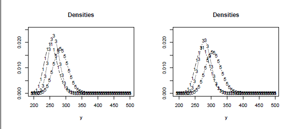
the random effect bi refers to the person and δ0 j accounts for the effect of days. It is not assumed that the mean is a linear function of days, as is common in typical random effects models. Instead, the basic variation of responses over repeated measurements is captured in the parameters δ0 j . The parameters δj account for possible heterogeneity of variances. The log(y) function, which makes the dependent variables follow a log-normal distribution, shows slightly better fit than the common normal distribution model. The log-likelihood was 872.96 with the log(y) function and 875.50 for the identity function (Gaussian distribution). Figure 1 shows the fitted densities for days 1, 3, 5, and 9 for bi = 0 and bi = 1. The latter value is approximately the same as the estimated standard deviation of the random coefficients, which was 1.08. It is seen that the distributions have quite different forms and variances vary across days. The mean reaction time as well as the variances increase over days of sleep deprivation.
Reaction time for days 1, 3, 5, and 9 of sleep deprivation for bi = 0 (left) and bi = 1 (right).
Various regression models have been proposed for continuous bounded data in the form of rates and proportions that take values in the interval (0, 1), see, for example, Kieschnick and McCullough (2003) and Bonat et al. (2019). Also mixed model versions for repeated measurement have been developed, in particular the simplex mixed model (Qiu et al., 2008) and beta mixed models (Bonat et al., 2015).
Let us more generally consider the case where 
Instead of
While simple terms for means and variances of the dependent variable can be found only for simple threshold functions as the linear one, it is straightforward to show that for any (non-decreasing) transformation function g(y) means and expectations of the transformed variables g(Yij) are given by

see Proposition 2 for a proof. That means the mean of the responses is a linear function of covariates and variances can vary over measurements.
Densities for predictor are
with binary predictor
and
, a = 0, b = 10; left: bi = 0; right: bi = 0.5; drawn line: xi = 0, dashed line: xi = 1.
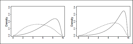
To illustrate the restriction to intervals generated by properly chosen thresholds functions, Figure 2 shows the obtained distributions if F(.) is the normal distribution, the predictor is
Discrete data come in two forms, with infinite support and finite support. We will consider first the case of infinite support and then the case where the response is in categories. In the latter, typically only an ordinal scale level is assumed for the dependent variable.
Random effects models for count data
Let the responses be counts, that is, Yij takes values from
In the mixed threshold model, the discrete density or mass function is given by
Parameter estimates for epilepsy data (p-values given in brackets).
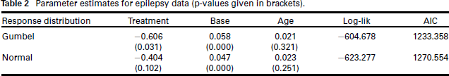
Parameter estimates for epilepsy data (p-values given in brackets).
A threshold function that ensures that the responses have support 0, 1, … is the shifted logarithmic threshold function

The resulting model is as flexible as models that account for overdispersion. In particular, the varying slopes δj make it very flexible and able to account for changes in distributional shape over measurements.
Epilepsy data
The response in the data set epil from R package
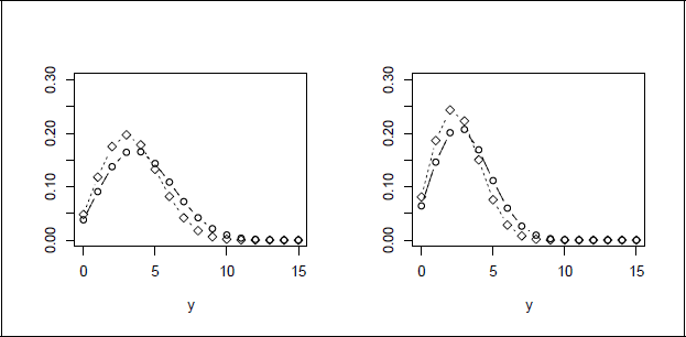
In the study, the most interesting effect is the treatment effect. For illustration Figure 3 shows the densities for period, 2 and 4 for placebo (left) and treatment (right) when using the Gumbel distribution, The other variables were chosen by bi = 0, base = 20, age = 20, diamonds indicate period four, circles period two. It is seen that treatment distinctly reduces the number of seizures.
The threshold model fits much better than the Poisson model, which yields log-likelihood −651.8071 and AIC 1313.614. It also fits better than the more general negative binomial model, which yielded log-likelihood −609.711. AIC values of the Gumbel threshold model and the negative binomial model are comparable (AIC for negative binomial model: 1231.423). Fitting of the Poisson and the negative binomial model was done by using the R package
Let Yij take values from {1, …, k} and assume that categories are ordered. The typical mixed model for this type of data is the cumulative mixed model considered among others by Jansen (1990) and Tutz and Hennevogl (1996) for univariate random effects. It has the form

with ordered intercepts
Densities for epileptics data with bi = 0, base = 20, age = 20; left: placebo, right: treatment, diamonds indicate period four, circles period two.
The model is equivalent to the threshold model

with the special choices
However, the model (3.2) without restrictions is more general than the simple cumulative model (3.1). In the simple cumulative model, the thresholds
Since the range of outcomes is bounded, similar threshold functions as in the case of bounded continuous data should be used. We use the logit type function

with a < 1 but close to 1, b = k.
An advantage of using a threshold function of the form
Fears data
As an illustrating example, we consider data from the German Longitudinal Election Study (GLES). The data originate from the pre-election survey for the German federal election in 2017 and are concerned with political fears. The participants were asked: ‘How afraid are you due to the …’: (1) refugee crisis? (2) global climate change? (3) international terrorism? (4) globalization? (5) use of nuclear energy? The answers were measured on Likert scale from 1 (not afraid at all) to 7 (very afraid).
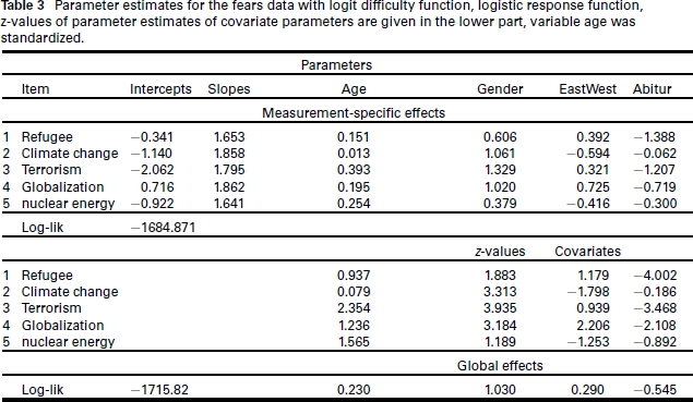
We fitted a discrete threshold with logistic response function and logit difficulty function including covariates, gender (1: female; 0: male), standardized age in decades, EastWest (1: Eastern German countries/former GDR, 0: Western German countries/former FRG) and Abitur (high school degree for the admission to the university, 1: yes, 0: no). Table 3 shows the estimates of item parameters. The parameters given are the intercept and the slope of the difficulty function
The model fits better than the common cumulative model (3.1), in which thresholds do not depend on j. By default the package
A strength of the threshold model is that dependent variables can be of various types. It allows for some of the measurements to be continuous while others are binary, ordinal or given as counts. Also the combination of continuous measurements with differing support can be modelled in a joint random effects model. There have been some approaches to joint modelling of different types of responses in specificsettings, see, for example, Ivanova et al. (2016) with a focus on ordinal variables or Loeys et al. (2011), where a joint modelling approach for reaction time and accuracy in psycholinguistic experiments has been proposed. However, no general random effects model that allows to combine different types of responses seems available.
The flexibility of threshold models to account for various types of measurement, is due to the general form of the model. Since the same model form, which specifies
Parameter estimates for the fears data with logit difficulty function, logistic response function, z-values of parameter estimates of covariate parameters are given in the lower part, variable age was standardized.
Parameter estimates for the fears data with logit difficulty function, logistic response function, z-values of parameter estimates of covariate parameters are given in the lower part, variable age was standardized.
Sleep data
As an illustrative example, let us again consider the sleep deprivation data. Instead of using the average reaction time per day in all 10 measurements, the last two measurements were transformed to ordered categorical data. More concretely, the interval (200, 500), which covers the reaction times, has been divided into six equidistant intervals and responses were coded as 1, …, 6 according to the responses in intervals. For the first eight measurements, the logarithmic threshold function has been chosen, and they are specified as continuous. For the last two measurements, the logit threshold function has been chosen and the measurements are specified as discrete with values 1, …, 6. The fitting of the model with normal response function yielded log-likelihood −768.597, which has to differ from the likelihood of the model with continuous responses considered earlier (−875.50) since now a combination of continuous and discrete distributions is assumed.
However, the variation of reaction times over days remains essentially the same. Figure 4 shows the densities for days 1, 3, 5 for bi = 0 (left) and bi = 1 (right). They are practically the same as the densities given in Figure 1, which shows the densities if all variables are considered as continuous.
Reaction time for days 1,3,5 of sleep deprivation for bi = 0 (left) and bi = 1 (right) for mixed responses.
A general form of the threshold function term is given by 
For continuous measurement j the density is

where 
For discrete data with 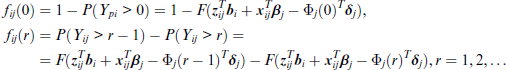
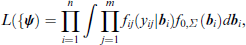
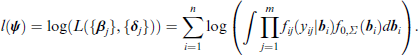
When assuming that random effects are normally distributed with mean zero and covariance matrix Σ the marginal log-likelihood has the form
where
The corresponding log-likelihood is given by
Maximization of the marginal log-likelihood can be obtained by using the Gauss–Hermite quadrature, as used, for example, by Anderson and Aitkin (1985), Rodríguez (2008) and Gueorguieva (2001). The Gauss–Hermite quadrature is typically based on the standardized random effects 
where ⊗ is the Kronecker product and
Then, the log-likelihood for the standardized random effects 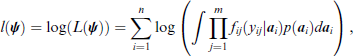
where p(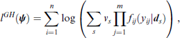
where
By building the derivatives to obtain the score function
An alternative is the adaptive Gauss–Hermite quadrature, which typically is more efficient and needs fewer quadrature points to obtain a good approximation, see Liu and Pierce (1994) and Rabe-Hesketh et al. (2005). A further alternatively is the EM algorithm, which was considered for mixed models among others by Bock and Aitkin (1981) and Anderson and Aitkin (1985). Overviews on inference tools for generalized mixed models are found in Jiang and Nguyen (2007) and McCulloch and Searle (2001).
It has been demonstrated that the threshold model is very versatile and can be adapted to quite different distribution functions. Moreover, it can be used in the joint modelling of different responses in a straightforward way. Joint modelling has been used in particular in the modelling of survival times and longitudinal data, see, for example, Hsieh et al. (2006). Mixed model approaches that are able to handle continuous, binary and ordinal responses can be based on a latent multivariate normal distribution. Goldstein et al. (2009) typically use the normal distribution only when modelling continuous responses.
We used marginal estimation based on integration methods, but alternative estimation from the toolbox of mixed models could be used. Regularization methods could be useful when trying to find sparser representations, for example by identifying those variables for which the effects do not vary over measurements. An overview on basic regularization method including boosting has been given by Hastie et al. (2009), and strategies to select those effects that do not vary over measurements have been considered, for example, by Tutz (2025).
The class of mixed threshold models could be made even more flexible by letting the data decide which threshold function is appropriate. In particular, B-splines as considered extensively by Eilers and Marx (2021) could be useful, which has been demonstrated by Tutz (2022) in the item-response setting without covariates.
Alternative flexible regression models that are in common use are quantile regression approaches and generalized additive models for location, scale and shape (GAMMLSS). Extension of quantile regression approaches that include random effects has been considered Koenker (2004) and Geraci and Bottai (2007) and Hsieh et al. (2006) but with a focus on continuous data for which quantile regression is most appropriate. Random effects within the GAMMLSS have been considered briefly in Stasinopoulos et al. (2024).
R programs that can be used to fit models by maximization of the marginal log-likelihood are available on github (
Footnotes
Appendix
For simplicity, let the model be given in the form
where
Where
Proof: For linear threshold function the threshold model has the form
which has the density
Thus, the mean is given by
With
where
The variance is given by
where
Proof: The mean is given by
With
since
The variance is given by
Acknowledgements
I want to thank the associate editor and two unknown reviewers for their helpful comments.
Declaration of Conflicting Interests
The author declared no potential conflicts of interest with respect to the research, authorship and/or publication of this article.
Funding
The author received no financial support for the research, authorship and/or publication of this article.