
Abstract
A novel approach is proposed for analysing multilevel multivariate response data. The approach is based on identifying a one-dimensional latent variable spanning the space of responses, which then induces correlation between upper-level units. The latent variable, which can be thought of as a random effect, is estimated along with the other model parameters using an EM algorithm, which can be seen in the tradition of the 'nonparametric maximum likelihood' estimator for two-level linear (univariate response) models. Simulations and real data examples from different fields are provided to illustrate the proposed methods in the context of regression and clustering applications.
Keywords
Introduction
When data possess a repeated measures structure, such as pupils nested within schools, or longitudinal measurements of individuals over time, the use of random effects to account for the ensuing correlations is now a commonplace technique. Specifically, the idea is to equip each upper-level unit with a random intercept which is shared by all lower-level units pertaining to it, and which induces the required correlations.
While these methods are well-developed and well-understood, and well supported by statistical software, they are typically restricted to univariate response scenarios. When the space of responses is multivariate, it is however not very clear how to actually adopt the idea mentioned above: Should there be a single or multiple random effects per upper-level unit, or in other words, shall the random effect distribution also be multivariate, and in either case, what is the shape of this distribution and how to estimate its parameters?
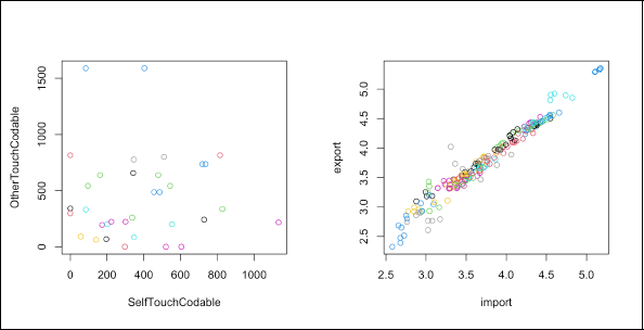
Before we begin with presenting our answer to these questions, we will briefly outline three examples for such problems which will serve as case studies later in this exposition. First in research on the effects of maternal mental health on prenatal movements in fetuses (Reissland et al., 2021), two touch movement types of twin fetuses were recorded during 4D ultrasound scans: self touch (the fetus touching itself) and other touch (the fetus touching the other twin). Figure 1 (left) shows the scatter plot of the two response variables symbolized by values of the upper-level variable 'mother'. The objective is to investigate the effect of maternal mental health (depression, stress and anxiety) onto the movement profile of twins, taking the correlation of the measurements of fetuses belonging to the same mother into account.
Left: Fetal twins' touch movements data, coloured by mothers. Right: Import and export data, coloured by countries.
Left: Fetal twins' touch movements data, coloured by mothers. Right: Import and export data, coloured by countries.
Second we consider data from the OECD (Organisation for Economic Co-operation and Development, 2023b) concerning trade in goods and services, providing country-wise percentages of imports and exports in relation to the overall GDP in 44 countries, for the time period between 2018 and 2022, during which between 3 and 5 observations are available for each country. Figure 1 (right) visualizes the data where the observations from the same country have the same colour. This can be considered as a multivariate repeated measures scenario, with unbalanced measurement occasions, and without covariates. We are particularly interested in clustering the countries with respect to their overall export/import activity relative to GDP size, taking within-country correlations across the repeated measurements into account. In recent related work, albeit employing a different methodology involving hidden Markov models, Pennoni et al. (2024) propose an algorithm for selecting the most important variables to cluster and classify countries by socio-economic development.
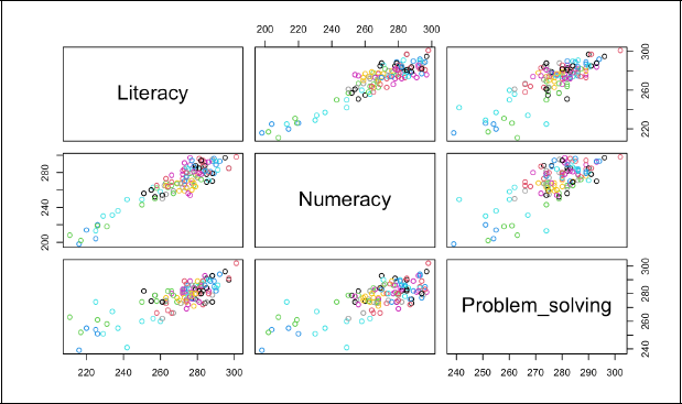
Third we consider the Programme for the International Assessment of Adult Competencies (PIAAC) survey of adult skills, carried out in 2011 and 2012 by the OECD. The PIAAC survey was designed to assess the proficiency of adults in the key information-processing skills of literacy, numeracy and problem solving (in technology-rich environments). All three skill types are provided on a continuous scale ranging from 0 to 500. For our analysis, we extracted from the PIAAC explorer (
Pairs plot of PIAAC data, coloured by countries.
We provide a modelling approach which will allow us to tackle the problems above, taking into account both the multivariate and the multilevel character of the outcome data. The approach is based on Zhang and Einbeck (2024a)’s latent variable model for dimension reduction and simultaneous clustering of highly correlated data, requiring only a single, one-dimensional random effect term. This paper develops the upheaval of that approach to two-level scenarios which is required to be able to deal with repeated measures data. We will give equal importance to the applications of clustering (of upper-level units) and multivariate regression for two-level data.
Some related model classes have been developed in the wider context of item response theory, most notably latent class models (Goodman, 1974). These models are commonly used for the clustering of observed multivariate categorical data (such as questionnaire outcomes on Likert scales) into latent classes. An obvious difference to our methodology is that in latent class models the response variables are categorical rather than continuous. A multilevel version of latent class models was developed by Vermunt (2003). A model selection procedure for deciding the number of latent classes at both levels is proposed by Lukočiené et al. (2010). Gnaldi et al. (2016) introduced a multilevel version latent class-item response theory model applied for educational data in which the collected response variables are dependent of each other. The latent class analysis also allows the inclusion of covariates; Di Mari et al. (2023) proposed a two-step estimator for the multilevel latent class model in which two categorical random effects are used to account for both the upper and lower-levels, allowing for clustering of the latent classes on both levels. It remains the case that due to the restriction on categorical outcomes, latent class models cannot be applied or compared with the situations dealt with in this work. However, it should not be left unstated that continuous-outcome versions of multilevel latent class models have also been developed, and are available in specialized commercial software such as Latent GOLD (Vermunt, 2008). Further related work includes Masci et al. (2022) who proposed a semiparametric mixed-effects model for multinomial data with hierarchical structure, in which a discrete random effect distribution is used to obtain the marginal density, and Bartolucci et al. (2011) who proposed a multilevel extension of latent Markov Rasch model and applied this on educational data with three-level structures. Verbeke et al. (2014) gave a general overview over longitudinal models for multivariate outcome data.
The structure of this paper is as follows. In Section 2 we introduce the proposed two-level model for multivariate response data. In Section 3, we present an EM algorithm for the proposed model, resembling the nonparametric maximum likelihood method. Section 4 shows simulation results that demonstrate the performance and accuracy of this algorithm for the estimation of model parameters. Section 5 provides real data examples that illustrate the main applications of our model, including the fitting of a multivariate response model resulting in reduced standard errors, the construction of league tables and the clustering of upper-level units based on the fitted model.
Some additional simulation results and complementary information have been relegated to the supplementary material. R Codes of the implemented methods, as well as of several of the presented examples, are available in R package mult.latent.reg, which is available on CRAN (Zhang and Einbeck, 2024b).
We consider a scenario where multivariate data

where

the data grouping process is carried out on the upper-level, while the lower-level units within the same upper-level unit share a common random effect term
For the distribution of random effects
Likelihood and estimators
Let
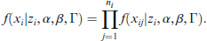
According to model (2.1), the marginal distribution of
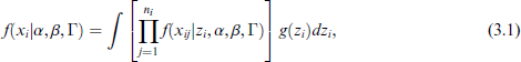
where
The marginal distribution can then be approximated as
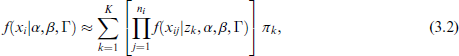
in which, by virtue of (2.2),

with the component-specific densities
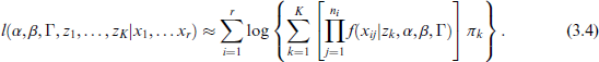
Now, the
Building on equation (3.2), the approximated marginal log-likelihood can be obtained as
In preparation of the EM algorithm (e.g., Dempster et al., 1977) to be used for the parameter estimation, we define by
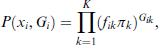
where for simplicity of notation we here used
Hence, we obtain the complete log-likelihood,
which may take values in
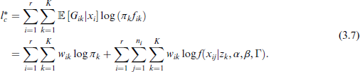
Plugging the expression for
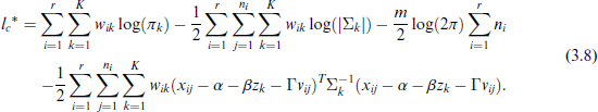
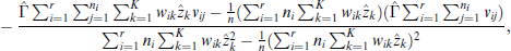
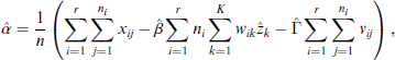
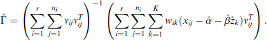
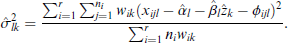
By taking partial derivatives of
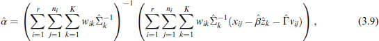

The solution for

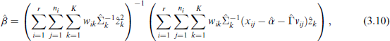
We furthermore find the general solution for

for

We note that this set of equations (3.9) to (3.14) is rather impractical to use directly, because the equations depend on each other in a complex manner, they involve multiple inversions of the estimated matrices

To avoid potential identifiability issues, certain restrictions are imposed on the model. First, we enforce
The resulting EM algorithm, which makes some further simplifications which are however of computational rather than model-related character, is presented in the next subsection.
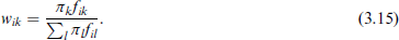
We have the following expectation (E) and maximization (M) steps resulting from the previous considerations.

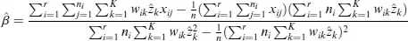
with the estimator for
These four equations are then iterated for a small number of times between each other, where the
This completes the M-step, and the procedure continues with the E-step (3.15).
Several options for selecting starting values have been implemented in the R package mult.latent.reg, which we described in Zhang and Einbeck (2024c). The required number of iterations is usually small, so that automated assessment of convergence is not necessary. The implementation in mult.latent.reg uses by default 20 iterations, which is generally sufficient. It is worth noting that due to the sequential nature of the updates within the M-step, this algorithm can be considered an ECM algorithm, for which convergence is, however, still guaranteed (Meng and Rubin, 1993). Choosing the number of mixture components K is a model selection process. Here, we use the AIC
Evaluate the accuracy of parameter estimation
We first conduct a simulation study to examine the accuracy of our parameter estimation using the simplified update expressions for the EM algorithm as described in Section 3.2. Another objective of this simulation is to investigate whether an increase in the number of upper- or lower-level units will effectively reduce the variance of the parameter estimates. We simulate data from bivariate two-level scenarios with a single covariate, where the number of mixture components is K = 2. We first consider a scenario with
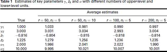
Estimates of key parameters
and
with different numbers of upper-level and lower-level units.
Estimates of key parameters
and
with different numbers of upper-level and lower-level units.
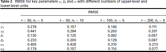
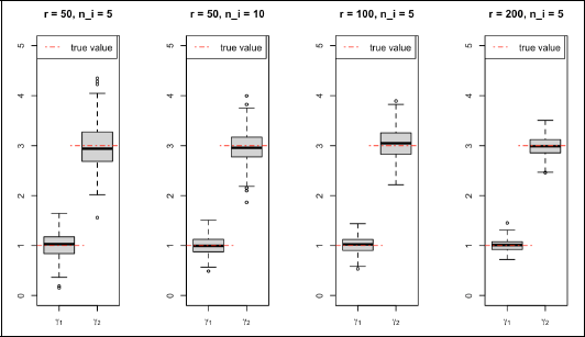
For the estimation from the simulated data, we also use K = 2. The effect of misspecifying K is considered in the supplementary materials. The simulation results, which are presented in Tables 1 and 2 and Figure 3, indicate that the true parameters are well estimated, and when we increase the number of upper-level units, the parameters' RMSE decreases stronger than when increasing the number of lower-level units. Note that, for a univariate parameter
RMSE for key parameters
and
with different numbers of upper-level and lower-level units.
Estimates of key parameter
with different number of upper-level and lower-level units.
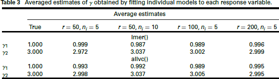
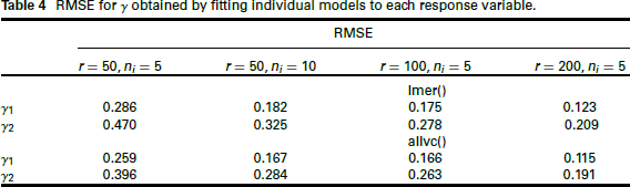
We also compare the
Averaged estimates of
obtained by fitting individual models to each response variable.
RMSE for
obtained by fitting individual models to each response variable.
Further analyses concerning the impact of misspecification of the number of mixture components and the random effect distribution are relegated to the supplementary material B and C. In brief, these simulation results confirm that the regression parameter
Analyses of case studies
In this section we analyse the real data sets from our case studies briefly introduced in Section 1. We focus on regression in the first case study and on clustering in the second case study, while in the third case study both regression and clustering are of interest.
Fetal twins' touch movements
The data set considered here was originally collected for research on the effects of maternal mental health on prenatal movements in twins and singletons (see Reissland et al., 2021). Since we are interested in a joint modelling of the two touch dimensions 'self touch' and 'other touch', we work here with slightly reduced data where the singletons are omitted (because singletons can't touch the 'other' twin). In the remaining twins' data, from 14 mothers who were pregnant with twins, 11 mothers were available for one scan and 3 were available for two scans, that is, in total there are 34 observations. Besides the two touch movement types, at the ultrasound scan appointment, the mothers' mental health status was collected on three variables: depression, perceived stress scale and anxiety. The data set as used in this case study is available as twins_data from R package mult.latent.reg.
For our analysis of the twins data set, we consider the two types of touches, self touch and other touch, as a bivariate response, and include the three mental health variables as covariates into model (2.1). Under this model, the observations within upper-levels (we consider each mother as an upper-level unit) share a common, mother-specific, random effect
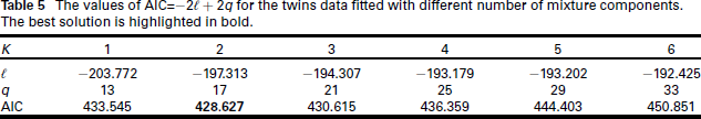
An examination of the AIC values across different values of
The values of
for the twins data fitted with different number of mixture components. The best solution is highlighted in bold.
The values of
for the twins data fitted with different number of mixture components. The best solution is highlighted in bold.
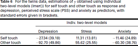
For the twins data, estimations of
obtained using individual two-level models (Imer()) for self touch and other touch as response and depression, perceived stress scale (PSS) and anxiety as predictors, with standard errors given in brackets.
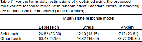
For the twins data, estimations of
obtained using the proposed multivariate response model with random effect. Standard errors (in brackets) are obtained via the bootstrap (1000 replicates).
The considered data set provides country-wise percentages of imports and exports, measured in million USD, in relation to overall GDP, for 44 countries, between 2018 and 2022. A varying number of observations has been available for different countries during this time. Specifically, Australia, Japan, Korea, Mexico, New Zealand, Turkey, the United States, China and Colombia have four observations each, while India, Russia and Brazil have three observations each. The remaining countries have five observations each. The data are extracted from the OECD website (Organisation for Economic Co-operation and Development, 2023b) and are available as trading_data in R package mult.latent.reg. In our analysis, the logs of imports and exports constitute a bivarate response variable, with
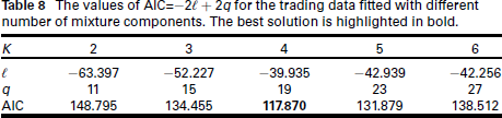
Fitting a bivariate response model of type (2.1), but without covariate, the minimum AIC is attained for
The values of
for the trading data fitted with different number of mixture components. The best solution is highlighted in bold.
The values of
for the trading data fitted with different number of mixture components. The best solution is highlighted in bold.
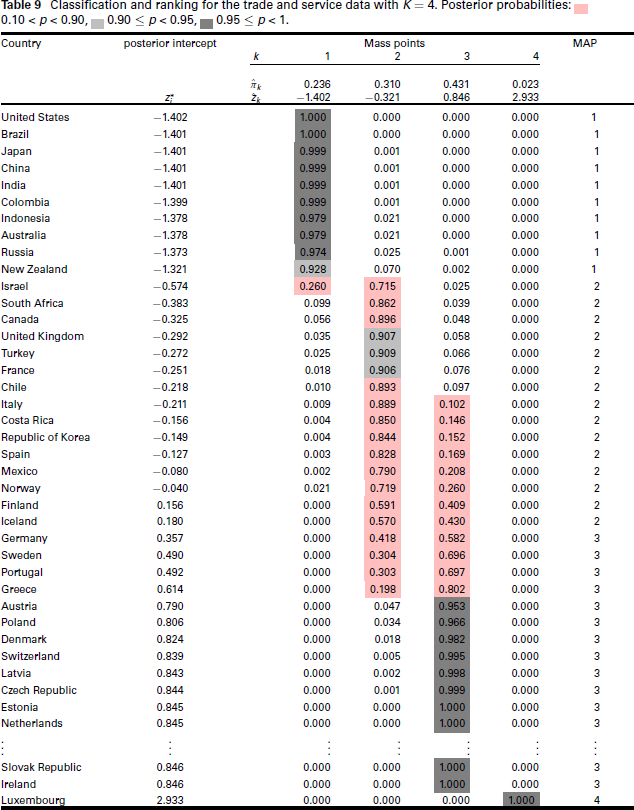
A sensible way of clustering the observations is to follow the MAP rule, that is, each upper-level unit (country) i is assigned to the cluster k to which it belongs with the largest probability
Classification and ranking for the trade and service data with
. Posterior probabilities:
.
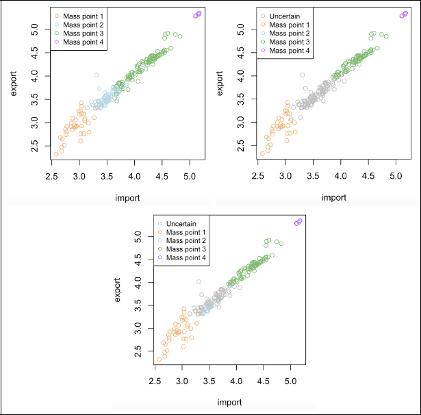
Clustering of the imports and exports data; top left using the MAP rule; top right with 95% confidence; bottom with 90% confidence. Note that three to five observations correspond to each country.
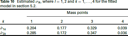
The second mass point
Estimated
, where
and
for the fitted model in section 5.2.
We note that neither the ranking (by posterior intercepts) nor the clustering (by the MAP rule) gives clear evidence on how well two countries, or two clusters, can actually be distinguished. However, the posterior probabilities available in the inner part of Table 9 help us to provide a principled way of doing so. If the largest posterior probability of the observation exceeds a certain level of confidence, say 0.95, it is clustered into that specific cluster with 95% confidence. That is, it can be robustly distinguished from observations (countries) that are allocated to other mass points at this level of confidence. This enables us to produce a 'robust' clustering of countries, as illustrated in Figure 4 top right. For example, Luxembourg is classified to the highest mass point 4 with a probability of 1, and it can be reliably distinguished from countries such as Ireland, Slovak Republic, …. Austria that all have a posterior probability >0.95 of belonging to mass point 3. Conversely, all countries for which the largest posterior probability is less than 0.95 are considered an uncertain observation that does not belong to any specific mass point, coloured as grey points in Figure 4 top right. This specifically concerns the countries of France, Turkey and the United Kingdom with their largest probabilities being below 0.95. At this level of confidence, the second mass point is eradicated entirely. However, changing the confidence level to 90% allows a robust clustering of these countries to mass point 2, as shown in Figure 4 bottom. Further conclusions could be drawn with careful reasoning: for instance, even under a 95% level of confidence, all countries from Greece to the United Kingdom can be robustly distinguished from both mass points 1 and 4, as they feature >95% probability mass between them. They just cannot be robustly distinguished between mass points 2 and 3 at that level.
We have seen that different levels of confidence lead to different 'confidence-adaptive' allocations of observations to clusters. While the most appealing choices of the confidence level for this purpose appear to be 1 (certain allocation), 0.95 and 0.90 (as illustrated), values down to even 0.5 could be of interest in certain situations as they would ensure a more certain allocation than the MAP estimate. It is also noteworthy that, as we have seen by the example of cluster 4, which, according to Table 9, only consists of one element, the size of a subpopulation is not of relevance for it being robustly clustered.
We now analyse the PIAAC data set, where literacy, numeracy and problem solving constitute a three-variate response, and gender and employment status serve as two covariates. Again this is a two-level model, with 30 countries defining the upper-level. The lower-level is defined through the different combinations of the covariate factor levels within each country; that is, there are four lower-level 'observations' for each country corresponding to the average score for this combination of covariates. More details about the survey and its design are provided in part D of the supplementary material and on the OECD website (Organisation for Economic Co-operation and Development, 2023a). It important to point out at this point that, in the analysis provided in here, no adjustment for country-wise variations in sampling design was undertaken, unlike for instance in the work by Hämäläinen et al. (2017) who fitted survey-weighted logistic models to PIAAC problem-solving scores.
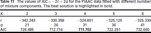
Using the methodology devised in this article, an examination of AIC values across different values of
The values of AIC
for the PIAAC data fitted with different number of mixture components. The best solution is highlighted in bold.
The values of AIC
for the PIAAC data fitted with different number of mixture components. The best solution is highlighted in bold.
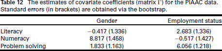
The estimates of covariate coefficients (matrix Г) for the PIAAC data. Standard errors (in brackets) are obtained via the bootstrap.
We can distinguish two countries in terms of their cluster membership if they fall with 95% confidence into two different mass points. In Table 13, all countries from New Zealand to Hungary are assigned with
Classification and ranking for the PIAAC data using model
with
. Posterior probabilities:
.
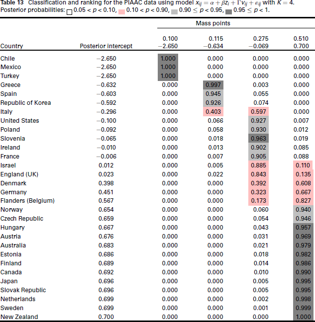
Note that it is not possible to determine a comparative ranking among countries belonging to the same mass point, for example, we cannot say that Japan has performed better than Canada. We also cannot robustly conclude that England (UK) or even Flanders (Belgium) have performed better than the United States, since they all share at least 5% probability mass with mass point 3.
We have provided a novel methodological approach for the inclusion of a random effect into multivariate response models, based on the NPML method for mixture models. The proposed approach enables us to accurately estimate covariate effects under the presence of correlations between response variables. Crucially, such correlations impact the standard errors of parameter estimates, as observed in our simulation studies and real data applications. It should however be noted that under this methodology, no analytic calculation of the standard errors is possible, hence requiring us to resort to bootstrap techniques.
Another advantage of the proposed methodology is in providing the matrix of posterior probabilities produced alongside the estimation process, as well as in calculating posterior random effects, based on the fitted model. We have demonstrated how these can be used for model-based clustering along the direction of the latent subspace and conditional on covariate values. The clustering can be performed either directly based on the maximum a posteriori (MAP) rule or can be driven by a user-specified degree of confidence in the cluster allocation, allowing for fine-grained insights into the separability of upper-level units on the scale of their posterior random effect. As suggested by a referee, entropy measures could potentially be used to assess the uncertainty of posterior probabilities, which in our context would correspond to values
Computationally, the proposed method can be regarded as the multivariate extension of the allvc function available in R package npmlreg (Einbeck et al., 2018). We here focused on the Gaussian errors assumption for the response model and used the nonparametric maximum likelihood approach to handle the marginal density of
Footnotes
Acknowledgements
We would like to thank Professor Nadja Reissland, Head of the Fetal and Neonatal Research Lab at the Department of Psychology, Durham University, for sharing the twins data which we used for our analysis in Section 5.1, and Dr Nick Sofroniou for helpful suggestions in the preparation of this project. We would also like to thank the three reviewers for their constructive and insightful comments.
Declaration of conflicting interests
The authors declared no potential conflicts of interest with respect to the research, authorship and/or publication of this article.
Funding
The authors received no financial support for the research, authorship and/or publication of this article.
Supplementary material
References
Supplementary Material
Please find the following supplemental material available below.
For Open Access articles published under a Creative Commons License, all supplemental material carries the same license as the article it is associated with.
For non-Open Access articles published, all supplemental material carries a non-exclusive license, and permission requests for re-use of supplemental material or any part of supplemental material shall be sent directly to the copyright owner as specified in the copyright notice associated with the article.