
Abstract
Feedforward neural networks (FNNs) can be viewed as non-linear regression models, where covariates enter the model through a combination of weighted summations and non-linear functions. Although these models have some similarities to the approaches used within statistical modelling, the majority of neural network research has been conducted outside of the field of statistics. This has resulted in a lack of statistically based methodology, and, in particular, there has been little emphasis on model parsimony. Determining the input layer structure is analogous to variable selection, while the structure for the hidden layer relates to model complexity. In practice, neural network model selection is often carried out by comparing models using out-of-sample performance. However, in contrast, the construction of an associated likelihood function opens the door to information-criteria-based variable and architecture selection. A novel model selection method, which performs both input- and hidden-node selection, is proposed using the Bayesian information criterion (BIC) for FNNs. The choice of BIC over out-of-sample performance as the model selection objective function leads to an increased probability of recovering the true model, while parsimoniously achieving favourable out-of-sample performance. Simulation studies are used to evaluate and justify the proposed method, and applications on real data are investigated.
Introduction
Neural networks are a popular class of machine-learning models, which pervade modern society through their use in many artificial-intelligence-based systems (LeCun, Bengio, and Hinton, 2015). Their success can be attributed to their predictive performance in an array of complex problems (Abiodun, Jantan, Omolara, Dada, Mohamed, and Arshad, 2018). Recently, neural networks have been used to perform tasks such as natural language processing (Goldberg, 2016), anomaly detection (Pang, Shen, Cao, and Hengel, 2021), and image recognition (Voulodimos, Doulamis, Doulamis, and Protopapadakis, 2018). Feedforward neural networks (FNNs), which are a particular type of neural network, can be viewed as non-linear regression models, and have some similarities to statistical modelling approaches (e.g., covariates enter the model through a weighted summation, and the estimation of the weights for an FNN is equivalent to the calculation of a vector-valued statistic) (Ripley, 1994; White, 1989). Despite early interest from the statistical community (White, 1989; Ripley, 1993; Cheng and Titterington, 1994), the majority of neural network research has been conducted outside of the field of statistics (Breiman, 2001; Hooker and Mentch, 2021). Given this, there is a general lack of statistically based methods, such as model and variable selection, which focus on developing parsimonious models.
Typically, the primary focus when implementing a neural network centres on model predictivity (rather than parsimony); the models are viewed as 'black-boxes' whose complexity is not of great concern (Efron, 2020). It is perhaps not surprising, therefore, that there is a tendency for neural networks to be highly over-parameterized, miscalibrated, and unstable (Sun, Song, and Liang, 2022). Nevertheless, FNNs can capture more complex covariate effects than is typical within popular (linear/additive) statistical models. Consequently, there has been renewed interest in merging statistical models and neural networks, for example, in the context of flexible distributional regression (Rügamer, Kolb, and Klein, 2024) and mixed modelling (Tran, Nguyen, Nott, and Kohn, 2020). However, statistically based model selection procedures are required to increase the utility of the FNN within the statistician's toolbox.
Traditional statistical modelling is concerned with developing parsimonious models, as it is crucial for the efficient estimation of covariate effects and significance testing (Efron, 2020). Indeed, model selection (which includes variable selection) is one of the fundamental problems of statistical modelling (Fisher and Russell, 1922). It involves choosing the 'best' model, from a range of candidate models, by trading pure data fit against model complexity (Anderson and Burnham, 2004). As such, there has been a substantial amount of research on model and variable selection (Miller, 2002). As noted by Heinze, Wallisch, and Dunkler (2018), typical approaches include significance testing combined with forward selection or backward elimination (or a combination thereof); information criteria such as Akaike information criterion (AIC) or Bayesian information criterion (BIC; Schwarz, 1978; Akaike, 1998; Anderson and Burnham, 2004); and penalized likelihood such as LASSO (Tibshirani, 1996; Fan and Lv, 2010).
In machine learning, due to the focus on model predictivity, relatively less emphasis is placed on finding a model that strikes a balance between complexity and fit. Looking at FNNs in particular, the number of hidden nodes is usually treated as a tunable hyperparameter (Bishop et al., 1995; Pontes, Amorim, Balestrassi, Paiva, and Ferreira, 2016). Input-node selection is not as common, as the usual consensus when fitting FNNs appears to be similar to the early opinion of Breiman (2001): 'the more predictor variables, the more information'. However, there are some approaches in this direction, and a survey of variable selection techniques in machine learning can be found in Chandrashekar and Sahin (2014). Nevertheless, typically, the optimal model is usually determined based on its predictive performance, such as out-of-sample mean squared error (OOS), which can be calculated on a validation dataset. Unlike an information criteria, out-of-sample performance does not directly take account of model complexity.
When framing an FNN statistically, there are several motivating reasons for a model selection procedure that aims to obtain a parsimonious model. For example, the estimation of parameters in a larger-than-required model results in a loss in model efficiency, which, in turn, leads to less precise estimates. Input-node selection, which is often ignored in the context of neural networks, can provide the practitioner with insights on the importance of covariates. Instead, other feature importance measures are typically used such as the feature attribution methods described in Koenen and Wright (2024). Furthermore, eliminating irrelevant covariates can result in cheaper models by reducing potential costs associated with data collection (e.g., financial, time, energy). In this article, we take a statistical-modelling view of neural network selection by assuming an underlying (normal) error distribution. Doing so enables us to construct a likelihood function, and, hence, carry out information-criteria-based model selection, such as the BIC (Schwarz, 1978), naturally encapsulating the parsimony in the context of a neural network. More specifically, we propose an algorithm that alternates between selecting the hidden layer complexity and the inputs with the objective of minimizing the BIC. We have found, in practice, that this leads to more parsimonious neural network models than the more usual approach of minimizing out-of-sample error, while also not compromising the out-of-sample performance itself.
The remainder of this article is structured as follows. In Section 2, we introduce the FNN model while linking it to a normal log-likelihood function. Section 3 motivates and details the proposed model selection procedure. Simulation studies to investigate the performance of the proposed method, and to compare it to other approaches, are given in Section 4. In Section 5, we apply our method to real-data examples. Finally, we conclude in Section 6 with a discussion.
Feedforward neural network
Let
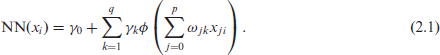
As we aim to frame FNNs as an alternative to other statistical non-linear regression models (i.e., used on small-to-medium sized tabular data sets relative to the much larger data sets seen more broadly in machine learning), and due to the universal approximation theorem (Cybenko, 1989; Hornik, Stinchcombe, and White, 1989), we are restricting our attention to FNNs with a singlehidden layer. The parameters in Equation 2.1 are as follows:
Given our assumption that

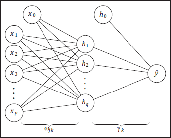
Neural network architecture with p input nodes and q hidden nodes.
where
The calculation of a log-likelihood function allows for the use of information criteria when selecting a given model, and in particular, the BIC (Schwarz, 1978), BIC
To begin model selection, a set of candidate models must be considered. For the input layer, we can have up to
Proposed approach
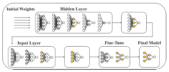
We propose a stepwise procedure that starts with a hidden-node selection phase followed by an input-node selection phase. (We find that this ordering leads to improved model selection.) This is, in turn, followed by a fine-tuning phase that alternates between the hidden and input layers for further improvements. The proposed model selection procedure is detailed in Algorithm 4 (which relies on Algorithms 1–3), and a schematic diagram is provided in Figure 2. It is also described at a high level in the following paragraphs.
Model selection schematic. Nodes coloured grey are being considered in current phase. Nodes coloured gold represent optimal nodes in that phase to be brought forward to the next phase.
Model selection schematic. Nodes coloured grey are being considered in current phase. Nodes coloured gold represent optimal nodes in that phase to be brought forward to the next phase.
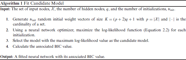
Fit Candidate Model
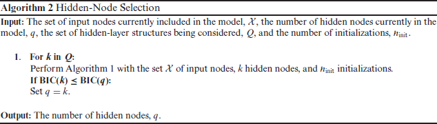
Hidden-Node Selection
Input-Node Selection
Model Selection
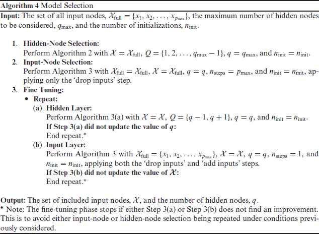
The procedure (Algorithm 4) is initialized with the full set of input nodes,
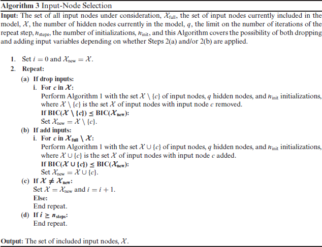
Once the hidden-node selection phase has concluded, the focus switches to the input layer (Algorithm 3); at this point, there are
Both the hidden layer and covariate selection phases are backward elimination procedures. Rather than stopping the algorithm after these two phases, we have found it fruitful to search for an improved model in a neighbourhood of the current 'best' model by carrying out some further fine tuning. This is done by considering the addition or removal of one hidden node (Algorithm 2 with
The particular order of the model selection steps described above has been chosen in order to have a higher probability in recovering the 'true' model, and to have a lower computational cost (see Section 4.1 for a detailed simulation). Note that choosing the set of input nodes requires a more extensive search than choosing the number of hidden nodes. There are more candidate structures for the input layer as you can have any combination of the nodes. Therefore, it is recommended to perform hidden-node selection first, to eliminate any redundant hidden nodes and decrease the number of parameters in the model, before performing input-node selection.
In order to justify and evaluate the proposed model selection approach, three simulation studies are used:
In the first two simulation studies, the response is generated from an FNN with known 'true' architecture. The weights are generated so that there are three important inputs,
The 'true' hidden layer consists of q = 3 hidden nodes, while we set our procedure to consider a maximum of
Simulation 1: model selection approach
This simulation study aims to justify the approach of the proposed model selection procedure, i.e., a hidden-node phase, followed by an input-node phase, followed by a fine-tuning phase; here, we label this approach as H-I-F. Some other possibilities would be: to start with the input-node phase (I-HF), to stop the procedure without fine tuning (either H-I or I-H), or to only carry out fine-tuning from the beginning (F). Descriptions of the considered model selection approaches are as follows (the proposed approach is highlighted in bold; round brackets indicate the reordering of the steps in Algorithm 4 required to achieve the approach):
H-I: Hidden-node selection phase, followed by input-node selection phase (Step 1 → Step 2). I-H: Input-node selection phase, followed by hidden-node selection phase (Step 2 → Step 1).
I-H-F: Input-node selection phase, followed by hidden-node selection phase, and then a finetuning phase (Step 2 → Step 1 → Step 3). F: Fine-tuning phase only (Step 3).
The objective function used for model selection is BIC, and each approach has
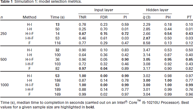
Simulation 1: model selection metrics.
Simulation 1: model selection metrics.
Time (s), median time to completion in seconds (carried out on an Intel® CoreTM i5-10210U Processor). Best values for a given sample size are highlighted in
Looking at the the model selection metrics, it is clear that the proposed H-I-F approach performs well, both in terms of selecting the correct set of input nodes and selecting the correct number of hidden nodes. Furthermore, the TNR is high, the FDR is low, and, as expected, we see that performance improves across all metrics with increasing sample size. From the results in Table 1, and from Figures 3 and 4, it is clear that the H-I-F approach performs best at recovering the true model structure.
Simulation 1: boxplots for TNR (the true negative rate for the input variables) for each method by sample size.

Simulation 1: boxplots for
(the number of hidden nodes selected) for each method by sample size. Median value highlighted in red. Dashed line indicates the true value of q.
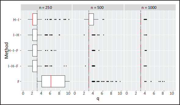
Comparing the methods without the fine-tuning stage in the boxplots, and looking at layerwise selection, the probability of selecting the correct structure is increased when that layer is selected in the second phase, e.g., input-node selection is best when it comes second (see H-I versus I-H in Figure 3). This suggests a relationship between the structure of the input and hidden layers (the probability of correctly selecting the structure of one layer increases when the other layer is more correctly specified). This is investigated further in Supplementary Material Section D. Therefore, H-I is likely better than I-H due to input-node selection being a more difficult task than hidden-node selection (determining the optimal set of input nodes versus the optimal number of hidden nodes), and, hence, it is favourable to perform it after hidden-node selection (given the number of hidden nodes is not substantially larger than the number of input nodes). This relationship between the structure of both layers can be handled by incorporating a fine-tuning phase after both the H and I phases are completed. Recall that the aim of fine tuning is to search for an improved solution in a neighbourhood of the current solution, where both H and I steps are carried out alternately (and include both backward and forward selections). Indeed, we see that the addition of the fine-tuning phase improves on H-I in the smaller sample sizes (in large part due to improved hidden-layer selection), but its addition does not greatly improve on I-H. Moreover, a boxplot for the computational time for each approach is provided in Supplementary Material Section E, and the addition of fine tuning only marginally adds to the computational expense. Overall, H-I-F is significantly better than I-H-F both in terms of computational expense and model selection. One may also consider only carrying out fine-tuning steps from the offset, which we denote by F. However, this does not perform as well as H-I-F at the smallest sample size and is more computationally demanding. From the above, the H-I-F approach is what we suggest as it leads to good model selection performance while also being the most computationally efficient approach.
This simulation study aims to determine the performance of using different objective functions when carrying out model selection. In particular, it aims to determine whether the use of an information criterion can improve the ability for the model selection procedure to recover the true model; this is compared to the far more common approach in neural networks of using out-of-sample performance. Three objective functions are investigated: BIC, AIC, and OOS. The AIC approach is the same as the proposed approach in Section 3.1, swapping BIC for AIC
Simulation 2: model selection metrics.
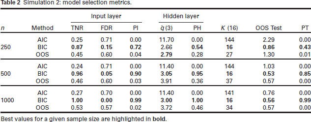
Simulation 2: model selection metrics.
Best values for a given sample size are highlighted in bold.
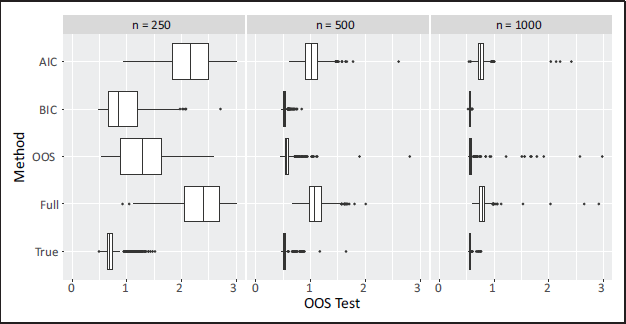
The results show that BIC far outperforms OOS and AIC in correctly identifying the correct FNN architecture. Using OOS as the model selection objective function almost never leads to correct neural network architecture being identified. This is due to the inability of the OOS to correctly identify and remove the unimportant covariates (TNR is always relatively low). Using AIC leads to even worse performance, and this is likely due to the weaker penalty on model complexity compared to BIC. It is also of interest to compare the approaches in terms of the size of the model selected and its out-of-sample performance. The median number of neural network parameters, K (note that the true value is K = 16), and the median OOS Test evaluated on a test set are reported. The OOS Test is computed on an entirely new dataset (20% the size of the training set) that the OOS-optimizing procedure was not exposed to. Interestingly, BIC-minimization leads to the lowest OOS values on the test data. This is particularly noteworthy since this is achieved using approximately half as many parameters as the OOS-minimization procedure. Boxplots highlighting the values of OOS Test and K are shown in Figures 5 and 6, respectively. Figure 5 also displays the OOS Test values for the true model (inputs
Simulation 2: boxplots for OOS Test for the models selected by each objective function; for comparison, the results for the true model (with inputs
and
) and the full model (with inputs
and
).
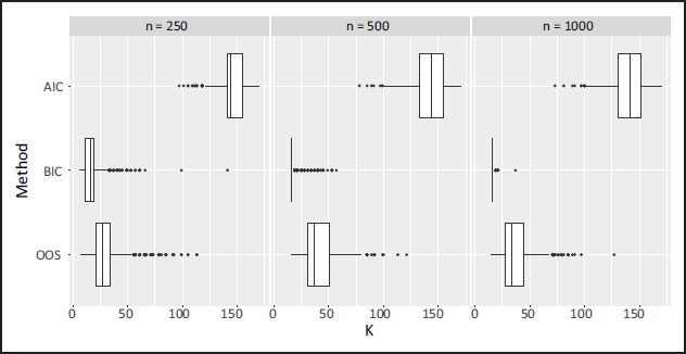
Simulation 2: boxplots for
(number of parameters) for the models selected by each objective function.
We have also compared our proposed BIC-based selection procedure to two commonly used strategies for dealing with overfitting, namely, weight decay and early stopping. The results are deferred to Supplementary Material Section H, where we have found that our proposed approach yields improved OOS Test values compared to these other two strategies.
For this simulation study, we investigate the performance of the proposed H-I-F model selection procedure on a dataset simulated from a data-generating process that is not a neural network:

where
From Table 3, we see that the proposed H-I-F procedure has a high TNR, a low FDR, and the true positive rate increases with the sample size; consequently, the probability of selecting the true set of covariates (PT) increases with the sample size. At the highest sample size, the out-of sample performance is very close to that of the correctly specified third order linear model (step lm-3). Although this true step-lm-3 model provides the lowest out-of-sample performance, its true negative and FDRs are relatively poor compared to the neural network, and, hence, the probability of selecting the true set of covariates does not approach one for the sample sizes we have considered. The selected step-lm-3 model does have fewer parameters on average than the neural network model (at n = 500 and n = 1000), but the step-lm-3 search is far more computationally intensive; this is due to the large number of possible interaction terms up to order three. It is important to note that the stepwise approaches for the linear models require the search space of models to be explicitly specified through the interaction and polynomial terms, and the performance of the misspecified (step-lm-2 and step-lm-1) approaches is very poor. In contrast, the proposed H-I-F selection approach does not require these terms to be explicitly specified, but still achieves very good out-of-sample performance since complex functional relationships and interactions are captured in a more automatic manner within the neural network structure.
Simulation 3: Comparison of proposed model selection approach for neural networks with stepwise model selection for linear models for the data-generating process given by Equation 4.1.
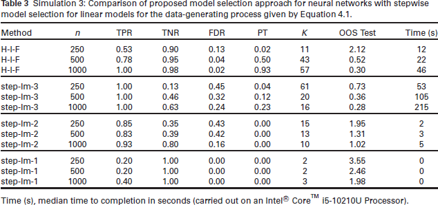
Time (s), median time to completion in seconds (carried out on an Intel ® CoreTM i5-10210U Processor).
Airbnb is an online marketplace that provides both short-term and long-term rentals. Data relating to the rental listings can be obtained from Inside Airbnb (
The dataset has been randomly split into a training set and test set with a 80%-20%- split, respectively, and all continuous variables have been standardized (based on the training data) to have zero mean and unit variance. The model selection procedure was implemented with
Our proposed procedure selects two hidden nodes and includes three covariates:
Dublin Airbnb: selected versus full model comparison.

Dublin Airbnb: selected versus full model comparison.
Dublin Airbnb: covariate effects and BIC differences.
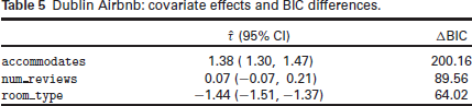
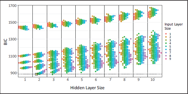
The selected model dropped six covariates (from a set of nine possible covariates). While the underlying selection procedure cannot guarantee that this model minimizes the BIC, and an exhaustive search through all sub-models is computationally expensive, we have nevertheless carried out such a search for the purpose of comparison. To this end, we fitted the model with all covariates included, all nine models that arise by dropping one of each of the covariates, all 36 models that arise when pairs of covariates are dropped, all 84 models that arise when triples of covariates are dropped, and so on, for each hidden layer size,
Figure 7 shows the BIC for each model where each point corresponds to a different input-layer hidden-layer combination; for comparison, the model selected by our procedure is indicated using a box. First, note that there is a subset of models with relatively large BIC values. Each of these models are missing the variables
Dublin Airbnb: BIC of models for different input-layer and hidden-layer combinations. Points are coloured according to the input layer size. The model selected by our procedure is enclosed in a box and the horizontal dashed line indicates the BIC for this model.
FNNs have become very popular in recent years and have the potential to capture more complex covariate effects than traditional statistical models. However, model selection procedures are of the utmost importance in the context of FNNs since their flexibility may increase the chance of over-fitting; indeed, the principle of parsimony is very common throughout statistical modelling more generally. Therefore, we have proposed a statistically motivated neural network selection procedure by assuming an underlying (normal) error distribution, which then permits BIC minimization. More specifically, our procedure involves a hidden-node selection phase, followed by an inputnode (covariate) selection phase, followed by a final fine-tuning phase. We have made this procedure available in our
Through extensive simulation studies, we have found that that (i) the order of selection (input versus hidden layer) is important, with respect to the probability of recovering the true model and the computational efficiency, (ii) the addition of a fine-tuning stage provides a non-negligible improvement while not significantly increasing the computational burden, (iii) using the BIC is necessary to asymptotically converge to the true model, and (iv) although the models selected using BIC have fewer parameters than those selected using out-of-sample performance, they have comparable, and sometimes improved, predictivity. We suggest that statistically orientated model selection approaches are necessary in the application of neural networks - just as they are in the application of more traditional statistical models - and we have demonstrated the favourable performance of our proposal.
In its current form, a limitation of the proposed procedure is that, due to its stepwise nature, it would be more computationally intensive when dealing with larger models and datasets. We expect that randomization and/or divide-and-conquer throughout the selection phases would be required in more complex problems involving many covariates and/or hidden layers, and adaptations may also be required for stochastic optimization procedures used on much larger datasets. Nevertheless, neural networks are still valuable in more traditional (smaller) statistical problems for which procedures such as ours will lead to more insightful outputs. Furthermore, the implementation of statistical approaches more broadly (such as uncertainty quantification and hypothesis testing) in neural network modelling will be crucial for the enhancement of these insights. This will be the direction of our future work.
Supplementary materials
Supplemental
Supplemental Material for A statistical modelling approach to feedforward neural network model selection by Andrew McInerney and Kevin Burke, in Statistical Modelling
Footnotes
Declaration of Conflicting Interests
The authors declared no potential conflicts of interest with respect to the research, authorship and/or publication of this article.
Funding
The authors disclosed receipt of the following financial support for the research, authorship, and/or publication of this article: This publication has emanated from research conducted with the financial support of Science Foundation Ireland under Grant number 18/CRT/6049. The second author was supported by the Confirm Smart Manufacturing Centre (
References
Supplementary Material
Please find the following supplemental material available below.
For Open Access articles published under a Creative Commons License, all supplemental material carries the same license as the article it is associated with.
For non-Open Access articles published, all supplemental material carries a non-exclusive license, and permission requests for re-use of supplemental material or any part of supplemental material shall be sent directly to the copyright owner as specified in the copyright notice associated with the article.