
Abstract
With the beginning of the COVID-19 pandemic, we became aware of the need for comprehensive data collection and its provision to scientists and experts for proper data analyses. In Germany, the Robert Koch Institute (RKI) has tried to keep up with this demand for data on COVID-19, but there were (and still are) relevant data missing that are needed to understand the whole picture of the pandemic. In this article, we take a closer look at the severity of the course of COVID-19 in Germany, for which ideal information would be the number of incoming patients to ICU units. This information was (and still is) not available. Instead, the current occupancy of ICU units on the district level was reported daily. We demonstrate how this information can be used to predict the number of incoming as well as released COVID-19 patients using a stochastic version of the Expectation Maximization algorithm (SEM). This, in turn, allows for estimating the influence of district-specific and age-specific infection rates as well as further covariates, including spatial effects, on the number of incoming patients. The article demon-strates that even if relevant data are not recorded or provided officially, statistical modelling allows for reconstructing them. This also includes the quantification of uncertainty which naturally results from the application of the SEM algorithm.
Introduction
Albeit its atrocity, in its aftermath, the COVID-19 pandemic has taught Germany, among many other countries, the shortcomings of inadequate data availability in its healthcare system. In fact, in Germany, while intensive care unit (ICU) occupancy was provided by the DIVI e.V. (2021), the numbers of newly hospitalized patients (incoming) and released patients (outgoing), either cured or deceased, has (until now) not been included in the database. This can be criticized since a relevant number, which measures the pressure of the disease on the healthcare system—the number of incoming patients—is not available to the public. We show, in this article, how to disentangle incoming and outgoing patients from pure occupancy data using statistical models. This, in particular, allows us to investigate how hospitalizations depend on time, age, and spatial factors.
We assume that admission to- and release of the ICU units follow Poisson distributions with inhomogeneous intensities. Consequently, the changes in ICU occupancy result from the difference between incoming and outgoing patients. This in turn gives the framework of the Skellam distribution, originally introduced by Skellam (1948). The distribution is described as resulting from the difference of two independent Poisson distributed random variables. This distributional approach has been used in different settings. For instance, in sports statistics Karlis and Ntzoufras (2009) apply the distribution for modelling the goal difference in football games. In network analysis, Gan and Kolaczyk (2018) and Schneble and Kauermann (2022) look at network flows while Koopman et al. (2014) utilize the idea to model financial trades. Further application areas include image analysis when comparing intensity differences of pixels, see for example, Hwang et al. (2007), Hwang et al. (2011) or Hirakawa et al. (2009). Extensions towards bivariate Skellam processes are provided for example, in Genest and Mesfioui (2014), see also Aissaoui et al. (2017). A general discussion on the Skellam distribution and its application fields is provided in Tomy and Veena (2022). In this article, we provide an application of the Skellam distribution for disentangling incoming and outgoing patients in ICUs.
The occupancy of ICU units was a central component of the COVID-19 pandemic. Numerous tools have been developed for forecasting the number of patients who require ICU admission, see for example, Grasselli et al. (2020), Goic et al. (2021), Murray (2020) or Farcomeni et al. (2021) to just mention a few. Our focus in this article is not primarily on prediction but on investigating the risk of admission and how this depends on the infection rates and further covariates, including spatial components. To do so we assume that the number of incoming and released patients comes from an inhomogeneous Poisson process, but we only observe the difference between incoming and released patients, leading to a Skellam distribution. Treating incoming and released patients as missing data, allows us to simulate the patient flows (stochastic E step) and refit the model (M step). Parameter estimation in the Skellam distribution is cumbersome due to its numerically complex form of the likelihood function, which requires the use of the Bessel function. Even though these are implemented in standard software packages, we refer to Schneble and Kauermann (2022), who report some numerical instabilities in the case of parameters at the boundary of the parameter space. We also refer to Lewis et al. (2016) or Aissaoui et al. (2017) who pursue moment-based estimation. In this article, we aim to use implemented routines to achieve stability. In fact, the data can be rewritten as a missing data constellation, which itself suggests the use of an EM algorithm. We here use the Stochastic Expectation Maximization (SEM) algorithm and present it as a suitable and numerically stable alternative to available estimation routines. Originally proposed by Celeux et al. (1996), the stochastic version of the EM algorithm gained interest in recent years, in particular in mixture models, see for example, Noghrehchi et al. (2021). We also refer to Nielsen (2000) for asymptotic results on the algorithm. The EM algorithm relates the estimation to a missing data problem, which is easily described. We assume that instead of the complete data with incoming and outgoing patients, we only observe the changes in occupancy of ICUs. In other words, the exact number of incoming and outgoing is missing. Replacing these missing numbers iteratively with simulated numbers, based on the current estimates of the model, provides the stochastic version of the ‘E’-step. This, in turn, leads to full data, which allows for standard maximum likelihood estimation of two Poisson processes—-the M step. The algorithm is easily implemented, and Rubin’s rule, Rubin (1976), provides inference statements.
A particularly interesting attribute that this approach provides is the simplification of the initial complexity of the problem. We are able to break our problem down from a fairly complex distributional assumption, with respect to deriving an association between the infection rates and the number of incoming and outgoing patients, to land at essentially two iteratively updated generalized additive models (GAMs) with simulated responses, each response simultaneously sampled from a joint distribution, comprised of the product of two Poisson distributions. This allows us to not only circumvent rather cumbersome calculations and modifications of the first and second derivative of the Skellam distribution, as, for example, shown by Schneble and Kauermann (2022) but also almost effortlessly interpret the association between the number of incoming and outgoing patients and the infection rate.
The article is structured as follows; in Section 2, we give a detailed data description. In Section 3, we elaborate on the model approach to our problem, while in Section 4, we will provide the results of our model approach. A simple simulation exercise to validate our findings can be found in Section 5, and in Section 6, we conclude our article which also includes a discussion of the shortcomings of our approach.
Data description
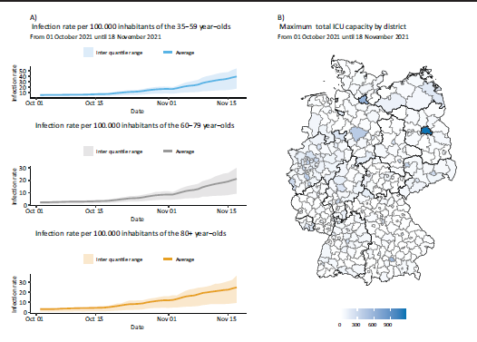
The database for our analyses consists of two main components; data on COVID-19 infections and data on the ICU occupancy of COVID-19 patients. The infections and the ICU occupancy are collected by the German health care departments, recorded by the Robert Koch Institute (2021) (RKI), the German federal government agency and scientific institute responsible for health reporting and disease control, and published by the RKI and DIVI e.V. (2021), respectively. We here focus on data during the fourth infection wave in Germany, that is, from the 2nd October 2021 until the 17th November 2021, though the method is readily extendable to other time frames, so long that the data included are subject to homogeneous testing or lock down strategies. We visualize the average infection rates over all districts in Figure 1 (left-hand side).
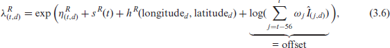
A: Summary over all districts of the infection rate per 100.000 inhabitants by age group, ‘45–59’ year-olds, ‘60–79’ year-olds and ‘80+’ year-olds displayed by date, from the 1 October 2021 until the 18 November 2021, B: The maximum capacity of ICU beds per given district over the time span from the 1 October 2021 until the 18 November 2021 by district.
A: Summary over all districts of the infection rate per 100.000 inhabitants by age group, ‘45–59’ year-olds, ‘60–79’ year-olds and ‘80+’ year-olds displayed by date, from the 1 October 2021 until the 18 November 2021, B: The maximum capacity of ICU beds per given district over the time span from the 1 October 2021 until the 18 November 2021 by district.
The RKI collects and publishes data on infections on a daily basis. Due to privacy protection, the RKI aggregates the number of COVID-19 patients, ICU occupancy and general hospital admission of patients infected with COVID-19 over NUTS3 districts, European Commission (2021), but separates by demographic groups. These namely are the age categories; ‘0–4’ year-olds, ‘5–14’ year-olds, ‘15–34’ year-olds, ‘35–59’ year-olds, ‘60–79’ year-olds and ‘80+’ year-olds and the sex; ‘male’, ‘female’ and ‘not disclosed’. For the purpose of this analysis, the infections are aggregated over the age groups. The data were directly downloaded through the ArcGIS website, Robert Koch Institute (2021). The infection rates per 100.000 inhabitants are then calculated as a weekly average for each age group. For each district, the infection rate is averaged over the seven days immediately preceding the respective observed day change in ICU occupancy.
The data on ICU occupancy is also collected by the RKI and published by DIVI. These data are also on a district level, however, the occupancy can only be differentiated by the number of beds occupied by patients infected with COVID-19, by the number of beds occupied by patients not infected with COVID-19 and the number of empty beds, the sum of which is the overall ICU capacity in a given district on a given date. We solely take the COVID-19 ICU-patients into account and visualize the ICU data for one day in Figure 1 (right-hand side).
Conveniently, both data sets can also be found in the daily updated GitHub repository maintained by the RKI, Robert Koch Institute (2023). We take a closer look at the infection rates by age group in the supplementary material.
Assumption
Let


The explicit modelling of the intensities
With these definitions, we can now define the difference

Assuming independence for the number of incoming and outgoing ICU COVID-19 patients together with (3.1) and (3.2) leads to a Skellam distribution Skellam (1948).

Before we derive how to estimate the two intensities in (3.4) we want to discuss the suitability of the distributional assumptions. Note that the approach relies on independence of
There was, however, relocation of patients if local hospitals reached the edge of capacity. This followed a national plan, called ‘Kleeblattkonzept’, literally translated as clover-leaf-concept, see Pfenninger et al. (2022). This also implies that some ICU patients are not local.
We also want to add a comment given by the referee, in that a Skellam distribution also results in a more general setup. Assume that we have noisy data in that incoming and released patients have an additive shift. That is instead of
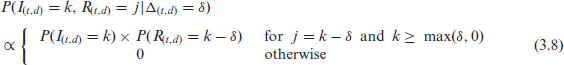
Finally, the intensities

where
Finally, we impose the standard identifiability constraints, that is, that both
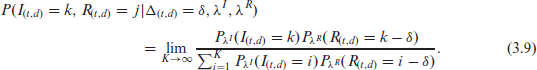
Instead of maximizing the Skellam likelihood, as done for instance in Schneble and Kauermann (2022), we pursue an EM algorithm, with the E-step replaced by a simulation step, leading to the stochastic EM algorithm, as discussed in Celeux et al. (1996). The approach has the advantage, that estimation can be carried out iteratively using implemented procedures and, even more importantly, we directly obtain predicted values for the incoming and released patients, which are the quantities of interest. Note that we observe

with the additional constraints that both,
with
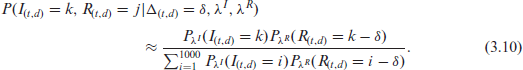
We approximate this numerically by assuming that either
Numerically this is easily carried out and allows to simulate data pairs
Iterating between the two steps gives a stochastic version of the EM algorithm. Each simulation step provides an estimate, and following the classical EM algorithm, we can easily see that on average, we increase the (marginal) likelihood in each step. The outline of which is sketched in Figure A4, in the Appendix.
The results of the model which simulates from the joint probability distribution with K = 2.000, instead of K = 1.000, are shown in the supplementary material.
Unlike the EM algorithm, where calculating the variance of the estimates is not straightforward, and one typically relies on Louis’ formula Louis (1982), the stochastic version allows to take the uncertainty due to the missing data into account. The derivation shows similarities to Rubin’s formula for imputation, see Rubin (1976). Let the parameter vector of linear and smooth functions,
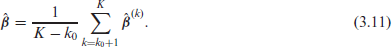
The variance is estimated via

where
A great advantage of our approach is that we can directly interpret the estimated association between the included covariates and the incoming patients and outgoing patients separately. To do so, we look at covariates containing information on the infection rates for each of the three age groups and the weekday effects. The estimated coefficients and their standard deviation, calculated based on Rubin’s formula, see Equation (3.12), are provided in Table 1. We use the last 300 runs to determine the coefficient estimates through their median, as well as their variance through the Equation (3.12). The estimates over the last 300 runs are shown through line plots in Figures A2 and A3 in the Appendix for the incoming and outgoing patients, respectively. We include extensions to the runs included in the analysis in the supplementary material. We find, however, that the inclusion of more runs will not result in a change in the estimated coefficients.
Estimated coefficients and standard deviations presented on the level of incoming and outgoing patients. The estimates are the exponential of the median of the coefficient estimates from the 200
th
run to the 500
th
run of the EM algorithm.
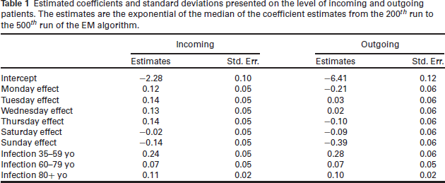
Estimated coefficients and standard deviations presented on the level of incoming and outgoing patients. The estimates are the exponential of the median of the coefficient estimates from the 200 th run to the 500 th run of the EM algorithm.
First, we look at the association between our covariates and the number of incoming and outgoing patients, as seen in the middle and right column of the output table, Table 1. Recall that the weekday effect is included in the model through a categorical variable, with Friday as its reference category. For the model estimating the number of incoming patients, keeping respectively all other variables constant, we can observe that there is an increased number of incoming patients on other weekdays, compared to Friday, whereas on the weekend, there is a decreased number of patients, compared to Friday. For outgoing patients, the behaviour is slightly different. On Monday, Thursday, Saturday, and especially Sunday, fewer patients are released compared to Friday. Conversely, Tuesday and Wednesday seem slightly increased.
The number of incoming and outgoing patients is positively associated with the infection rates of all age groups. Notably, the strongest effect exists for the infection rate of ‘35–59’ year-olds. This is interesting, bearing in mind that ‘60–79’ year-olds are the predominant age group DIV. We should, however, not omit that there is strong collinearity between the infection rates themselves which could affect our interpretability of the coefficients. More on the change of coefficients, when we look at different time frames over which the data is observed is discussed in the supplementary material.
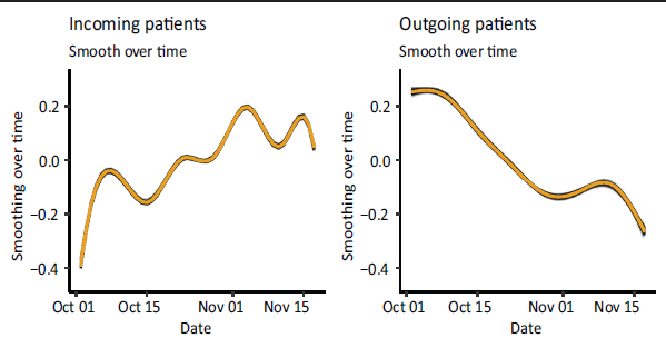
Recall further, that we included smooth functions to estimate both the spatial-, and the temporal effects. They are included to pick up on additional spatial and temporal structural dependencies. Let us first look at the smooth effects over time, as seen in Figure 2. The averaged smooth function over time for incoming patients (left-hand side) is generally increasing. Evidently, we can see some fluctuation and there seems to be a fortnightly rhythm within the overall trend. Here we observe an increase in the number of incoming patients for the first seven days, then a decrease in the following seven days, followed by a subsequent increase, and so forth. In contrast, as shown on the right-hand side of Figure 2, we see a general decrease in the number of outgoing patients without a biweekly rhythm.
Estimated smooth functions of all runs, over time, rendered by the GAMs estimating the number of incoming patients (left hand side) and outgoing patients (right hand side) over the last 300 runs.
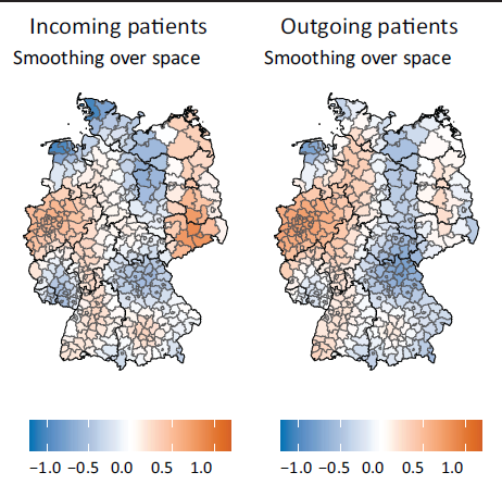
Finally, we look at the spatial effects for the incoming patients, see the left-hand side of Figure 3, and for the outgoing patients, shown with the right-hand side of Figure 3. There seems to be an increased level of incoming patients in Saxony (east Germany) and North Rhine-Westphalia (west Germany) and a slight increase around the larger cities of Germany (Frankfurt, Stuttgart, and Munich, south and southwest of Germany). We observe a similar structure in the spatial smooth function in the model estimating the outgoing patients, except for the strong increase around Saxony. Overall, we see clear spatial heterogeneity.
Estimated median smooth functions of the 200 th until the 500 th run over space rendered by the generalized additive models, estimating the number of incoming patients (left-hand side) and outgoing patients (right-hand side).
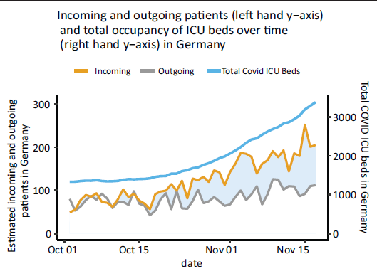
At last, we visualize in Figure 4 the estimated number of incoming and outgoing patients, summed up over the entirety of Germany, for the observed time frame. The left-hand axis scales the number of incoming and outgoing patients, whereas the right-hand axis scales the number of overall ICU patients with COVID-19. We see that the model picks up the somewhat constant occupancy, from the 1 October 2021, until the 17 October 2021, in Germany’s ICUs rather well, where the number of incoming and outgoing patients are estimated to be similar, if not equal. Thereafter, the number of ICU patients in the ICU increases, around this time, we also observe a higher estimated number of incoming patients than outgoing patients. It is not unusual for patients, especially the critically ill, to stay in the ICU for more than four weeks, making the divergence in estimation for the number of incoming patients and outgoing patients entirely plausible.
Estimated number of incoming and outgoing patients by date from the 1 October 2021 until the 18 November 2021, as well as the total number of COVID-19 patients in the ICUs of Germany.
With respect to model validation, we provide some additional analyses in the supplementary of the article. In particular, we look at serial correlation and show that due to the autoregressive component in the model, the Pearson residuals show no autocorrelated structure.
This section is aimed to investigate the goodness of fit of the modelling approach we chose a simple version to emulate the data used above. We use one covariate, randomly drawn from a normal distribution, whose mean and variance are taken from the observed mean and variance of the logged infection rates of ‘60–79’ year-olds. We choose this age group, as ‘60–79’ year-olds are the predominant group in the German ICUs during the fourth wave, see Robert Koch-Institut (2023). The coefficients for the simulation are chosen in a way such that the difference in the simulated incoming and outgoing patients is somewhat similar to the range of the difference in the observed incoming and outgoing patients, namely (-24,20) in the observed data. The incoming and outgoing number of patients are then simulated, outlined in Equation 5.1.


Here,
The estimated coefficients for twenty simulated data sets.
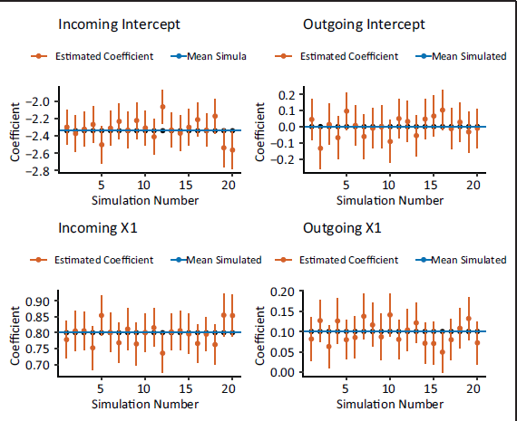
Overall, the simulation confirms that we are able to uncover incoming and outgoing patients from pure hospitalizations.
Overall, in this application of the SEM, we are not only able to simulate unobserved data but also estimate the association between the weekday effect and the infection rates and the number of incoming and outgoing patients in a simple and intuitive manner. We achieve some insight into the estimated association between the infection rates and the number of incoming and outgoing patients. Namely, the driving force of the estimated number of incoming and outgoing patients seems to be the infection rates of ‘35–59’ year-olds. Although we are not able to validate the predictions against the actual number of incoming and outgoing ICU patients, our findings seem to be mostly reasonable. Additionally, the SEM estimates the association of the simulated number of incoming and outgoing ICU patients and the simulated covariate well. In this situation, the SEM seems to be an appropriate application and allows us to gain a more complete picture of the COVID-19 pandemic, even when dealing with incomplete information.
Footnotes
Declaration of Conflicting Interests
The authors declared no potential conflicts of interest with respect to the research, authorship, and/or publication of this article.
Funding
We acknowledge the support of the Deutsche Forschungsgemeinschaft (DFG, Project KA 1188/13-1).
Appendix
Supplementary material
References
Supplementary Material
Please find the following supplemental material available below.
For Open Access articles published under a Creative Commons License, all supplemental material carries the same license as the article it is associated with.
For non-Open Access articles published, all supplemental material carries a non-exclusive license, and permission requests for re-use of supplemental material or any part of supplemental material shall be sent directly to the copyright owner as specified in the copyright notice associated with the article.