
Abstract
Fine-scale covariate rasters are routinely used in geostatistical models for mapping demographic and health indicators based on household surveys from the Demographic and Health Surveys (DHS) program. However, the geostatistical analyses ignore the fact that GPS coordinates in DHS surveys are jittered for privacy purposes. We demonstrate the need to account for this jittering, and we propose a computationally efficient approach that can be routinely applied. We use the new method to analyse the prevalence of completion of secondary education for 20-49 year old women in Nigeria in 2018 based on the 2018 DHS survey. The analysis demonstrates substantial changes in the estimates of spatial range and fixed effects compared to when we ignore jittering. Through a simulation study that mimics the dataset, we demonstrate that accounting for jittering reduces attenuation in the estimated coefficients for covariates and improves predictions. The results also show that the common approach of averaging covariate values in windows around the observed locations does not lead to the same improvements as accounting for jittering.
Keywords
Introduction
Fine-scale spatial estimation of demographic and health indicators has become commonplace (Burstein et al., 2019; Utazi et al., 2019; Local Burden of Disease Vaccine Coverage Collaborators, 2021). This article is focused on prevalences, which include many important indicators such as completion of secondary education, neonatal mortality, and vaccination coverage (Fuglstad et al., 2021). For low- and middle-income countries (LMICs), the household surveys conducted by the Demographic and Health Surveys (DHS) Program are a crucial data source. Geographic information in DHS data is given through GPS coordinates, which describe centres of clusters of households. However, cluster centres are randomly displaced by up to 10 km before being published in order to protect participants' privacy (Burgert et al., 2013). We refer to such small random displacements as jittering of the GPS coordinates.
In global health, it is common practice to ignore jittering and estimate risk using a standard geostatistical model with a binomial likelihood. The latent spatial variation in risk is modelled as the combination of raster- and distance-based covariates and a Gaussian random field (GRF). However, covariate values extracted from rasters can vary widely on the distance scale of jittering. Using the covariate value at the jittered location instead of the original location induces a non-standard form of measurement error (Gustafson, 2003). This may in turn lead to attenuation of effect estimates and errors in uncertainty. Furthermore, not accounting for the positional uncertainty for the GRF, artificially reduces estimated spatial dependency and may reduce predictive power as well (Cressie and Kornak, 2003; Fanshawe and Diggle, 2011; Fronterrè et al., 2018).
To address uncertainty in covariates, Perez-Heydrich et al. (2013, 2016) suggested (a) to use regression calibration in the context of distance-based covariates (Warren et al., 2016), and (b) to average spatial covariates within a 5 km buffer zone for continuous and categorical rasters. However, this approach does not address the issue of attenuation of associations. Fanshawe and Diggle (2011) proposed a Bayesian approach to account for positional uncertainty for the GRF, but did not propagate uncertainty in the covariates, and only used Gaussian likelihoods that are not applicable to prevalences. The approach was also computationally expensive, but Fronterrè et al. (2018) made the approach computationally efficient and demonstrated its applicability to analyse malnutrition based on DHS data.
Recently, Wilson and Wakefield (2021) formulated a full geostatistical model for DHS data that includes an observation model for the jittered GPS coordinates, and estimated the model with integrated nested Laplace approximations (INLA) (Rue et al., 2009) within Markov chain Monte Carlo (MCMC) (Gómez-Rubio and Rue, 2018). Their approach addresses the effect of positional uncertainty on both the spatial covariates and the GRF, but was computationally expensive with 1000 MCMC iterations requiring 52 hours in their simulation study. Altay et al. (2022) proposed a similar model as Wilson and Wakefield (2021), but used a more efficient inference scheme with computation time being measured in minutes instead of hours. Their approach was made possible through an approximation of the likelihood, the stochastic partial differential equations (SPDE) approach (Lindgren et al., 2011), and Laplace approximations through template model builder (TMB) (Kristensen et al., 2016).
The simulation study in Altay et al. (2022) revealed that small spatial ranges for the GRF or larger jittering than the DHS scheme were required to see substantial improvements with the new approach over ignoring jittering. Altay et al. (2022) focused on the impact of jittering on the GRF, and lacked raster- and distance-based covariates. Such covariates are far more variable at small spatial scales than a smoothly varying GRF. The aim of this article is to extend the approach in Altay et al. (2022) to a full generalized geostatistical model for prevalence, and to demonstrate that ignoring jittering can lead to attenuation of associations and reduced predictive power when analysing DHS data. We show this via a spatial analysis of the prevalence of secondary education completion among women aged 20-49 in 2018 based on the 2018 Nigeria DHS (NDHS2018) (National Population Commission - NPC and ICF, 2019).
In addition to the new approach, which adjusts for jittering, and the standard approach, which ignores jittering, we consider the common approach of averaging covariates in 5 km × 5 km windows around the provided GPS coordinates (Perez-Heydrich et al., 2013, 2016). The three methods cannot be compared with cross-validation since the true coordinates of the clusters are not known. Therefore, we construct a simulation study that mimics the NDHS2018 dataset to compare them in terms of their ability to estimate parameters and to predict risk at unobserved locations. We use bias and root mean square error (RMSE) to assess parameter estimation, and RMSE and continuous rank probability score (CRPS) (Gneiting and Raftery, 2007) to assess predictive ability.
We introduce the datasets and variables of interest in Section 2. Then, in Section 3, we describe the new approach that adjusts for jittering, and discuss its implementation. In Section 4, we evaluate parameter estimation and prediction with the different methods through a simulation study that mimics the prevalence of secondary education completion. Then, in Section 5, we demonstrate the differences between adjusting and not adjusting for jittering when analysing the prevalence of secondary education completion for women aged 20-49 in Nigeria. The article ends with discussion and conclusions in Section 6. The code used in the article can be found in the GitHub repository
Data sources and variables of interest
Our outcome of interest is completion of secondary education, which is an indicator of social wellbeing and life outcome (Lewin, 2008). Rates vary strongly between women and men, but also between urban and rural areas. According to UNESCO (2019), only 1 % of the poorest girls in low income countries will complete secondary education. If a girl completes secondary education, the risk of HIV infection is reduced by about 50 % (UNAIDS, 2022).
We consider the prevalence of secondary education completion for women aged 20-49 years in Nigeria in 2018. The lower bound was chosen because younger women may not have completed secondary education yet, and the upper limit was chosen since older women are not available in the DHS surveys. The year 2018 was chosen since this corresponds to the most recent DHS survey in Nigeria, NDHS2018.
Nigeria is an LMIC with a population of more than 200 million, and NDHS2018 has data collected from 1389 clusters with responses from 33,398 women aged 20-49, where 15,621 of them reported that they had completed their secondary education. In this article, we use the 1380 clusters with valid GPS coordinates, which have responses from 33,193 women aged 20-49 where 15,490 reported that they had completed their secondary education.
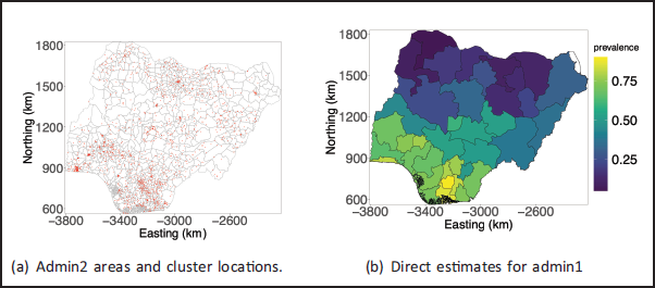
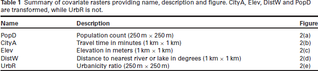
Figure 1(b) shows the direct estimates (Rao and Molina, 2015) computed based on the data and the survey design for the 36 states and one federal capital territory. The corresponding uncertainty is expressed through the coefficient of variation (CV). These 37 areas are the first administrative level (admin1), and the results show considerable variation between areas. The CVs increase when direct estimates are calculated at finer spatial scales due to observations needing to be distributed amongst more areas, resulting in smaller sample sizes per area. The second administrative level (admin2) for Nigeria, for example, consists of the 774 local government areas shown in Figure 1(a). The red dots in the figure indicate the 1380 clusters with GPS coordinates within Nigeria available in NHDS2018. The national boundary, admin1 boundaries and admin2 boundaries are based on GADM version 4.0 (GADM).
Maps of (a) admin2 areas and cluster locations for NDHS2018, and (b) admin1 areas with direct estimates.
Maps of (a) admin2 areas and cluster locations for NDHS2018, and (b) admin1 areas with direct estimates.
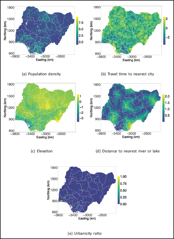
We expect the prevalence of completion of secondary education to be closely related to the access to educational resources, such as technological infrastructure, schools and teachers. We consider five spatial covariates: population count (PopD) (World Pop, 2022), travel time to nearest city (CityA) (Weiss et al., 2018), elevation (Elev) (National Oceanic and Atmospheric Administration, 2022), distance to nearest river or lake (DistW) (Natural Earth, 2012), and urbanicity ratio (Pesaresi et al., 2016). For UrbR, we scale the original covariate to be on a zero to one scale, and for the other four covariates, we use a log(1 + x)-transformation and then center and standardize the covariate rasters across the pixels. The information about the covariate rasters and figures is summarized in Table 1. The covariate rasters are available at different resolutions, and have not been resampled or aggregated to the same resolution since this would involve an extra preprocessing step that would induce misalignment error and potentially add ecological bias (Greenland and Morgenstern, 1989).
Summary of covariate rasters providing name, description and figure. CityA, Elev, DistW and PopD are transformed, while UrbR is not.
We aim to map spatial variation at a continuous spatial scale through a geostatistical model. A key challenge with using the above covariates is that the locations shown in Figure 1(a) are not the true locations. The true locations have been randomly displaced while respecting the admin 2 borders. This means that we can only imprecisely extract covariates from the rasters shown in Figure 2. The new method to account for the uncertainty in locations is described in Section 3.
Transformed covariate rasters for Nigeria.
Notation for DHS data
For a given country and DHS household survey,
Geostatistical model
Model for spatial variation in risk
We envision a spatially varying risk, 
where 
where
Unadjusted model
When jittering is ignored, the reported cluster locations 
where
Let 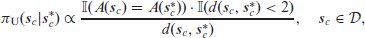
where
The jittering distributions 
where 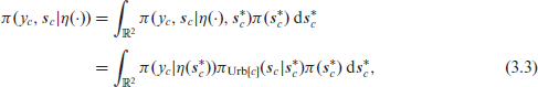
We assume linear covariate associations, and use the prior
Implementation
Inference scheme
The observation model in Equation (3.2) can be written as,

for

Two key components are combined for rapid inference: the SPDE approach to approximate the Matérn GRF (Lindgren et al., 2011), and Template Model Builder (TMB) for empirical Bayesian inference (Kristensen et al., 2016).
For each cluster
The SPDE approach (Lindgren et al., 2011) overcomes this issue by approximating the Matérn GRF that results in a sparse precision matrix. First, the area of interest is triangulated with a triangulation consisting of 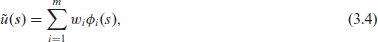
where
From Equation (3.4), the value at any location is a linear transformation
The SPDE is given by

where 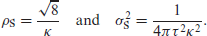
We implement the empirical Bayesian inference scheme by employing the built-in auto-differentiation and Laplace approximations of the TMB R package. Unlike sampling based MCMC methods, TMB uses numerical integration, through Laplace approximations, to perform inference. The auto-differentiation is used to speed up the Laplace approximations. See Kristensen et al. (2016) for the details.
In TMB, one can compute arbitrary likelihoods, and we can approximate the likelihood in Equation (3.3) through the integration scheme

where 
Based on the known jittering distribution, we construct the integration scheme with rings of integration points around each cluster center. The observed cluster center is the first integration point, and we use 5 and 10 rings for the clusters that are located within urban and rural administrative areas, respectively. Each ring consists of 15 angularly equidistant integration points.
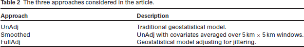
Throughout this article we consider the three approaches shown in Table 2. UnAdj denotes the traditional model that does not adjust for jittering, Smoothed denotes a model where the covariates have been averaged over
The three approaches considered in the article.
In this section, we evaluate the three models illustrated in Table 2 using a known data generating model, where the parameters correspond to FullAdj estimated based on completion of secondary education in Section 5, see Table 4. The data generating model is chosen to achieve realistic scenarios, and the aim is to evaluate accuracy in parameter estimation, and accuracy in predictive distributions. The key interest is how these accuracies vary across different strengths of the signal from the covariates.
We assume that the true spatial risk varies as

where
For each of the three scenarios, we generate
For observations, we follow the design of the NDHS2018 survey. We fix the number of clusters to
We fit the models UnAdj, Smoothed and FullAdj described in Section 3 using an intercept and the five covariates described above. The PC prior on the Matérn GRF is specified by
Parameter estimation is evaluated by computing the RMSE,
The simulation study was run on a computing server that operates on Linux (Ubuntu 20.04). The computing server has 28 cores (2X14-core Xeon 2.6GHz) and provides 256GB memory limit per user. It took on average 4 minutes to estimate the parameters
Table 3 shows the bias and RMSE for each of the parameters and covariate coefficients for SignalMed. The results show that UnAdj and Smoothed performs almost the same for
Bias and RMSE of parameter estimation for SignalMed.
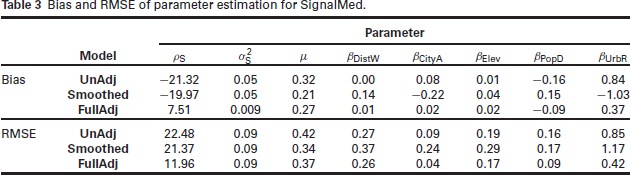
For example, the association with the urbanicity ratio of a 250 m x 250 m pixel and the urbanicity ratio of a 5 km x 5 km pixel are two different things. Additional tables for SignalLow and SignalHigh are found in Section 3 in the Supplementary Material.
Figure 3 shows boxplots of estimated
Box plots of estimated
and
for SignalLow, SignalMed and SignalHigh. The horizontal red lines show the true parameter value.
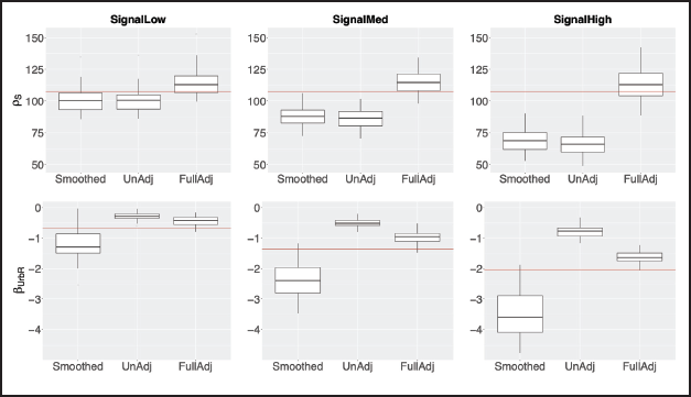
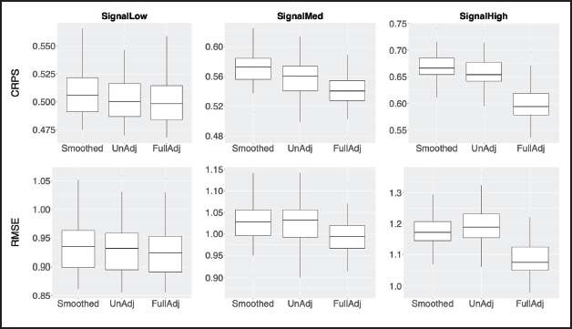
Figure 4 shows the variation in RMSE and CRPS across datasets for predictions. FullAdj and UnAdj perform almost the same in both predictive metrics for SignalLow, but FullAdj is slightly better for SignalMed, and substantially better for SignalHigh. This indicates that the stronger the signal of the spatial covariates, the larger the gain from adjusting for jittering. The figure also indicates that Smoothed does not have better predictive ability than UnAdj.
Box plots of CRPS and RMSE for predictions for SignalLow, SignalMed and SignalHigh.
In addition to the simulation study described above, we performed a simulation study with the true locations fixed to the observed locations of NDHS2018. The goal was to examine the predictive metrics for the specific spatial design of NDHS2018. There were only minor differences between this simulation study, and the one described above, and we, therefore, show these results in Section 2 of the Supplementary Material. This suggests that we should expect the unadjusted model to underestimate range, and lose predictive accuracy due to reduced association with the covariates.
In this section, we analyse the spatial variation in prevalence of completion of secondary education among 20-49 year old women in Nigeria in 2018 based on the NDHS2018 using the data sources described in Section 2. Our analysis has two aims. First, to map the fine-scale spatial variation in completion of secondary education for 5 km x 5 km pixels, and for the admin 1 areas. Second, to determine the associations between the spatial variation in risk and a set of explanatory spatial covariates.
The NDHS2018 has C = 1,380 clusters with jittered GPS coordinates available under the same jittering distribution as in Section 3.2. For all clusters, the jittering was restricted to stay within the correct admin2 area. In total, 33,193 women aged 20-49 years were interviewed and 15,490 of these had completed secondary education. We use the notation
We fit the models UnAdj, Smoothed and FullAdj described in Section 3 using an intercept and the five covariates described in Section 2. We use the PC prior on the Matérn GRF specified by
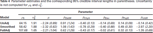
Table 4 shows the estimated parameters and their corresponding credible interval lengths (except for
Parameter estimates and the corresponding 95% credible interval lengths in parentheses. Uncertainty is not computed for
and
.
Parameter estimates and the corresponding 95% credible interval lengths in parentheses. Uncertainty is not computed for
and
.
For PopD and UrbR, there is a strong attenuation when jittering is ignored. The credible intervals for the coefficient of UrbR,
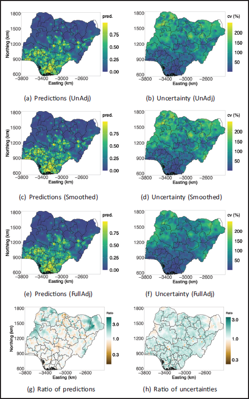
Figure 5 shows the
Rows 1, 2 and 3 are predicted risk and the CVs for UnAdj, Smoothed, and FullAdj, respectively. Row 4 shows ratios (UnAdj/FullAdj) of predictions and CVs.
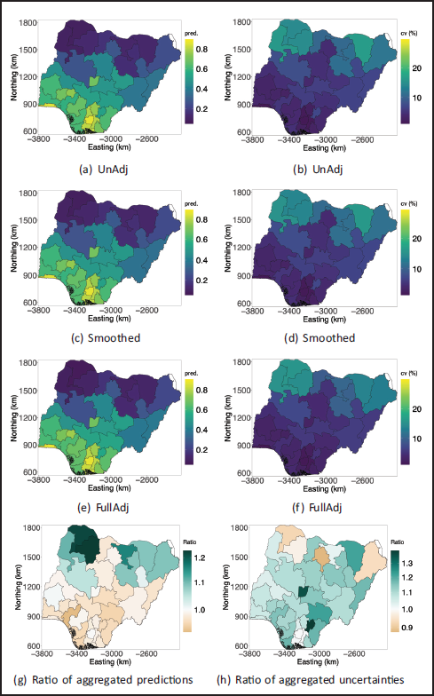
We aggregate point level predictions with respect to population density to produce areal estimates at the
Rows 1 and 2 are predicted risk and CVs for UnAdj and FullAdj respectively at the admin 1 level, and row 3 shows ratios (UnAdj/FullAdj) of predictions and CVs.
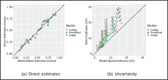
In Figure 7, we compare the areal estimates from the FullAdj model against direct estimates. Figure 7(b) shows that the FullAdj reduces uncertainty compared to the direct estimates, and Figure 7(a) shows that the estimates from FullAdj and the direct estimates are compatible with no unexpected deviations.
Comparison direct estimates and (areal) model-based estimates for (a) the mean, and (b) the coefficient of variations.
The ability to predict risk at unobserved locations for UnAdj, CovAdj and FullAdj cannot be compared with cross validation. If data is held-out from NDHS2018, we can only evaluate the models' ability to predict risk at a new jittered cluster with unknown true location. However, the simulation study in Section 4 indicates that FullAdj leads to an improvement in prediction if the data-generating model is the one estimated in this section.
Accounting for jittering substantially changed the parameter estimates for the geostatistical model for completion of secondary education among women aged 20-49 years. The simulation study demonstrated that these differences were linked to the strength of the signal of the spatial covariates when explaining the spatial variation. For strong signals, the associations were attenuated and the predictive power was reduced.
The most important aspect of jittering in the context of geostatistical models for DHS data is to account for the resulting uncertainty in covariates extracted from rasters or extracted based on distances. This induces measurement error that may lead to attenuation in associations between covariates and the responses. Some covariates such as sanitation practices and household assets can be known exactly (Burgert-Brucker et al., 2016), but these cannot be included when the goal is prediction since fine-scale rasters are not available.
In influential work such as Burstein et al. (2019) and Local Burden of Disease Vaccine Coverage Collaborators (2021), covariates are resampled to a
This article used uniform priors for the unknown true locations. One could expect including information about population density and urbanicity into the priors would produce more accurate inference. However, population density maps and urbanicity maps are also modelled surfaces with biases and uncertainties that are not well understood. This means that evaluation of the sensitivity to such maps would have to be investigated, and one would need a way to evaluate whether such a model works better.
The inference scheme uses empirical Bayes. It is possible to investigate methods such as INLA, but the implementation in the
When analysing completion of secondary education, we found that, for urbanicity, an effect size of 0 was contained in the
Supplementary material
Supplementary material for this article is available online.
Supplemental Material for Impact of jittering on raster- and distance-based geostatistical analyses of DHS data by Umut Altay, John Paige, Andrea Riebler and Geir-Arne Fuglstad, in Statistical Modelling
Appendix
Computational details
The application in Section 5 was run on a MacBook Pro (2.4GHz Quad-Core Intel Core i5 and 16 GB memory). For FullAdj, it took 7.8 minutes to estimate parameters, and 4.2 minutes to compute predictions.
A newly developed R-package GeoAdjust (Altay et al., 2023) is now available on CRAN for analysing DHS data while accounting for jittering in a more compact way, similar to the analysis in Section 5. The package provides a user-friendly functionality by isolating the user from
Footnotes
Declaration of Conflicting Interests
The authors declared no potential conflicts of interest with respect to the research, authorship and/or publication of this article.
Funding
The authors received no financial support for the research, authorship and/or publication of this article.
References
Supplementary Material
Please find the following supplemental material available below.
For Open Access articles published under a Creative Commons License, all supplemental material carries the same license as the article it is associated with.
For non-Open Access articles published, all supplemental material carries a non-exclusive license, and permission requests for re-use of supplemental material or any part of supplemental material shall be sent directly to the copyright owner as specified in the copyright notice associated with the article.